Computational Tools for Low-Temperature ... - CiteSeerX

22

Reviews in Mineralogy & Geochemistry Vol. 58, pp. 589-622, 2005 Copyright © Mineralogical Society of America

Computational Tools for Low-Temperature Thermochronometer Interpretation Todd A. Ehlers, Tehmasp Chaudhri, Santosh Kumar Department of Geological Sciences University of Michigan Ann Arbor, Michigan, 48109-1005, U.S.A. [email protected]

Chris W. Fuller, Sean D. Willett Department of Earth and Space Sciences University of Washington Seattle, Washington, 98195, U.S.A.

Richard A. Ketcham Jackson School of Geosciences University of Texas at Austin Austin, Texas, 78712-0254, U.S.A.

Mark T. Brandon Department of Geology and Geophysics Yale University New Haven, Connecticut, 06520-8109, U.S.A.

David X. Belton, Barry P. Kohn, Andrew J.W. Gleadow School of Earth Sciences The University of Melbourne Victoria 3010, Australia

Tibor J. Dunai Faculty of Earth and Life Sciences Vrije Universiteit De Boelelaan 1085, 1081 HV Amsterdam, The Netherlands

Frank Q. Fu School of Geosciences University of Sydney, NSW 2006, Australia and CSIRO Exploration and Mining, PO Box 1130, Bentley, WA, Australia

INTRODUCTION This volume highlights several applications of thermochronology to different geologic settings, as well as modern techniques for modeling thermochronometer data. Geologic interpretations of thermochronometer data are greatly enhanced by quantitative analysis of the data (e.g., track length distributions, noble gas concentrations, etc.), and/or consideration of the thermal field samples cooled through. Unfortunately, the computational tools required for a rigorous analysis and interpretation of the data are often developed and used by individual labs, but rarely distributed to the general public. One reason for this is the lack of a good 1529-6466/05/0058-0022$05.00

DOI: 10.2138/rmg.2005.58.22

590

Ehlers et al.

medium to communicate recent software developments, and/or incomplete documentation and development of user-friendly codes worth distributing outside individual labs. The purpose of this chapter is to highlight several user-friendly computer programs that aid in the simulation and interpretation of thermochronometer data and crustal thermal fields. Most of the software presented here is suitable for both teaching and research purposes. Table 1 summarizes the different programs discussed in this chapter, the contributing authors behind each program1, the computer operating system each program runs on, and the application or purpose each program is intended for simulating. The intent of this chapter is not to provide a user manual for each program, but rather an introduction to concepts and physical processes each program simulates. All software discussed here is freely available for non-profit applications and can be downloaded from http://www.minsocam.org/MSA/RIM/ under the link for Volume 58, Low-Temperature Thermochronology. This web page contains executable versions of the software, copyright information, example input and output data files, and, in some cases, additional documentation and user manuals. The availability of source code for modifying each program varies, and interested persons are encouraged to contact the leading contributor. Regular users of these programs are encouraged to contact the software contributor to receive software updates and bug fixes. Software updates will occasionally be posted on the MSA web server as well. Software users should be aware of the caveats associated with use of these programs2. The remainder of this chapter is dedicated to highlighting the functionality of each software package. Several items are discussed for each software package. These items include: (1) the intended application of each program and motivation behind its development, (2) the general theory and equations solved in the program, (3) the input required to run the program, and (3) the output generated.

TERRA: FORWARD MODELING EXHUMATION HISTORIES AND THERMOCHRONOMETER AGES Contributors: T. Ehlers, T. Chaudhri, S. Kumar, C. Fuller, S. Willett ([email protected]) The TERRA (Thermochronometer Exhumation Record Recovery Analysis) software simulates rock thermal histories and thermochronometer ages generated during exhumation. There are two linked modules to this program. The “Thermal Calculation” module calculates cooling histories for either 1D transient heat transfer with variable erosion rates, or 2D steady1

Suggested format for referencing software described in this chapter: Each computer program described in this chapter was developed by different contributors (Table 1). To assure each contributor receives appropriate credit for their contribution please include the contributor and software names in any citations used in publications. For example, programs in this volume could be cited in the following way, “We computed erosion rates using the program AGE2EDOT developed by M. Brandon and summarized in Ehlers et al. (2005).” If additional publications are available describing the software (e.g., HeFTy; Ketcham et al. 2005) please also reference those publications.

2 Caveats related to software use and distribution: There are two caveats associated with the software provided in this volume. (1) The software is provided as a courtesy to the broader scientific community and in some cases represents years of effort by the contributors. The software can be used free of charge for non-profit research, but persons with commercial or for-profit interests and applications should contact the contributors concerning the legalities of its use. (2) Although every effort has been made by the contributors to assure the software provided functions properly and is free of errors, no guarantee of the validity of the software and results calculated can be made. Thus, application of the software is done at the users own risk and the software contributors are not accountable for the results calculated.

Computational Tools

591

Table 1. Summary of software contributions. Program Name

Contributors

Application / Purpose

Operating Systems Supported

TERRA

T. Ehlers, T. Chaudhri, Forward modeling thermochronometer ages, S. Kumar, C. Fuller, apatite and zircon fission track and (U-Th)/He S. Willett

Windows®, Linux

HeFTy

R. Ketcham

Forward and inverse modeling apatite fission track, (U-Th)/He, vitrinite reflectance data

Windows®

BINOMFIT

M. Brandon

Calculate ages and uncertainties for concordant and mixed distributions of FT grain ages

Windows®

CLOSURE, AGE2EDOT RESPTIME

M. Brandon

Calculate effective closure temperatures, erosion rates, and isotherm displacement for several thermochronometer systems

Windows®

FTIndex

R. Ketcham

Calculated index temperatures and lengths of fission track annealing models

Windows®

TASC

D. Belton, B. Kohn, A. Gleadow

Fission track age spectrum calculations

Windows® (Excel®)

DECOMP

T. Dunai

Forward modeling (U-Th)/He age evolution curves

Windows®

4DTHERM

F. Fu

Thermal and exhumation history of intrusions

Windows®, Linux, Mac®

state heat transfer for user defined periodic topography and erosion rates. The “Age Prediction” module uses the thermal histories generated in the first module, or any other user defined thermal histories, to calculate cooling rate dependent apatite and zircon (U-Th)/He ages, and apatite and zircon fission track ages. The program is platform independent and runs on Windows® XP, and Linux® operating systems. Future releases of the program will run on the Macintosh® operating system as well. A graphical user interface (GUI) is provided for user input. However, the ageprediction program can also run without the graphical interface at the command line under the Linux® or DOS® operating systems if batch processing of multiple thermal histories from other, more sophisticated, thermal models is desired. The source code for these programs is available on request and written using C++ and Qt.

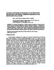
TERRA – 1D and 2D thermal history calculations The TERRA thermal calculation module is well suited for users to explore different erosion/exhumation scenarios and their influence on subsurface temperatures. The influence of different rates and durations of erosion, as well as topographic geometries, can be easily evaluated so users develop an intuition for crustal thermal processes. Figure 1 illustrates the user interface, or menu, for the calculation of 1D transient thermal fields during erosion. This program can be used to predict sample cooling histories for different user defined rates and durations of erosion. It is particularly useful for evaluating the transient evolution of subsurface temperatures and cooling histories during the early stages (e.g., first 5 m.y.) of mountain building and erosion. The program operates by solving the 1D transient advection-diffusion equation for a homogeneous medium with no heat production (for details,

592

Ehlers et al.

Figure 1. TERRA interface for calculation of 1D transient thermal histories for variable erosion rates.

see Eqns. 6 and 7 in Ehlers 2005). Rock thermal histories are recorded as they approach the surface. User defined inputs include thermal boundary conditions and material properties, model geometry, and rate of erosion. Several plots are generated from this program, including: (1) the thermal history of exhumed samples (Fig. 2), (2) geotherms at different time intervals (Fig. 2), and (3) the depth history of user defined temperatures (e.g., closure temperatures). The cooling history of a rock exposed at the surface is written to an output file for loading into the age prediction program. Figure 3 illustrates the TERRA user interface for calculating the steady-state 2D thermal field beneath periodic topography. This program can be used to determine the position of isotherms and rock cooling histories under uniformly eroding topography. This program is particularly useful for evaluating the curvature of closure isotherms beneath topography of different wavelengths and amplitudes and potential topographic effects on cooling ages. The program operates by solving the steady-state 2D advection-diffusion equation for a uniformly eroding medium with depth dependent radiogenic heat production and periodic topography (Manktelow and Grasemann 1997). User defined inputs include thermal boundary conditions,

Computational Tools

593

Figure 2. Example of TERRA predicted geotherms (top) and exhumed sample thermal history (bottom) plots from the 1D transient thermal calculation.

model geometry (topographic wavelength and amplitude), erosion rate, and material properties. Two plots are generated from this program: (1) The steady-state cooling history of rocks exposed between a ridge and adjacent valley bottom, and (2) the topography and steadystate position of user defined isotherms beneath the topography. Thermal histories of samples exposed between a ridge and valley are output to a file for loading into the age prediction program (see below). All plots generated in this 2D periodic topography and the 1D transient erosion menus have options to print or save the plot. Other options available in the plot windows include the ability to zoom in and out to different parts of the plot. The menus also include default input parameters to help users unfamiliar with common thermal properties of rocks use the programs.

594

Ehlers et al.

Figure 3. TERRA input window for calculating steady-state cooling histories beneath 2D periodic topography.

TERRA – thermochronometer age prediction The TERRA program also calculates predicted low-temperature thermochronometer ages from user defined thermal histories. Predicted ages for several thermochronometer systems are possible including: apatite and zircon (U-Th)/He ages and 4He concentration profiles across grains, multi-kinetic apatite fission track ages, and zircon fission track ages. Zircon fission track ages are calculated using an effective closure temperature. Figure 4 shows two example input ‘tabs’ for the TERRA age prediction module. The first step in using the age prediction module is to load in files with rock thermal and coordinate position (optional) histories. The thermal and coordinate history for either a single sample, or for multiple samples, can be loaded to calculate predicted ages. The ability of this program to load multiple thermal histories for batch processing predicted ages is particularly useful for interpreting cooling histories calculated from more complex 2D or 3D thermal models (e.g., Ehlers and Farley 2003, Ehlers et al. 2003). After a thermal history is loaded, any or all of the thermochronometer ages listed at the top of the window can be calculated.

Computational Tools

595

Figure 4. TERRA input windows for loading thermal history input files (top) and apatite (U-Th)/He age prediction (bottom). The window tabs for other thermochronometer systems have similar layouts.

The methods used for calculating each of the thermochronometer ages are as follows:

•

Apatite and zircon (U-Th)/He ages: (U-Th)/He ages are calculated by solving the transient spherical ingrowth diffusion equation for homogeneous distributions of U and Th, and temperature dependent diffusivity (e.g., Farley 2000; Reiners et al. 2004). The equation is solved using a spherical finite element model as described in Ehlers et al. (2001, 2003).

•

Apatite fission track ages: Apatite fission track ages are calculated using the mutikinetic annealing model of Ketcham et al. (1999, 2000). This model is similar to

596

Ehlers et al. the HeFTy program discussed later and accounts for variable annealing behavior as it correlates to etch pit width (Dpar). Apatite fission track ages are calculated following the approach developed by Fuller (2003).

•

Zircon fission track ages: Unlike apatite, a well developed annealing model for zircon fission tracks does not exist. As a consequence, TERRA calculates zircon fission track ages using an effective closure temperature (Dodson 1973, 1979; see also Brandon and Vance 1992; Brandon et al. 1998; and Batt et al. 2001). Zircon fission track ages are also calculated following the approach developed by Fuller (2003).

Calculated ages and coordinates of each sample (if provided in the input files) are written as output. Users can define their own kinetic parameters for (U-Th)/He and fission track age prediction, or use the default values to get started quickly.

HEFTY: FORWARD AND INVERSE MODELING THERMOCHRONOMETER SYSTEMS Contributor: R. Ketcham ([email protected]) HeFTy is a computer program for forward and inverse modeling of low-temperature thermochronometric systems, including apatite fission-track, (U-Th)/He, and vitrinite reflectance. Fission-track and (U-Th)/He calculations are described in Ketcham (2005), and vitrinite reflectance is calculated using the EasyRo% method of Sweeney and Burnham (1990). HeFTy can simultaneously calculate solutions for up to seven thermochronometers. In addition to data analysis, HeFTy can also be an instructional aid, as it allows easy, interactive comparisons among thermochronometric systems and their parameters. It reproduces and extends the functionality of AFTSolve (Ketcham et al. 2000), and is intended to fully replace that program. It runs on the Windows® operating system. Figure 5 shows an example screen from HeFTy, with one file window open. Each file window in HeFTy corresponds to a single sample or locality, which can have associated with it multiple thermochronometers. To create a model, use one of the 3 “new” buttons on the top left of the task bar: the first creates a “blank” model (no thermochronometers), the second creates an AFT model, and the third a (U-Th)/He model. Additional thermochronometers can be included by clicking on the “+” button and selecting the type desired. Up to seven thermochronometers can be added. For each thermochronometer, a new tab page is created, allowing model parameters to be changed and data to be entered for fitting. Whenever a model is added, this tab page is automatically brought to the front. To generate numbers, go to the “Time-Temperature History” tab. Clicking and dragging in the time-temperature history graph causes the forward model to run for all thermochronometers. Data to be compared to forward modeling results or fitted using inversion can be typed directly into the program interface, and tabular data (such as fission-track lengths and singlegrain ages) can be transferred from a table or spreadsheet using the clipboard (i.e., cutting and pasting). The easiest and most foolproof way to enter such data is using tab-delimited text files, which can be exported from any spreadsheet program. Included with the HeFTy distribution is the Microsoft Excel® file “Import templates.XLS”, which contains examples of all of the various input formats HeFTy supports. The inverse modeling module is accessed by clicking the button to the right of the “+” button. A new window comes up for controlling the inversion processing (Fig. 6), and mouse clicks and motions in the time-temperature history graph create box constraints through which inverse thermal histories are forced to pass. Constraints can overlap, although rules are enforced to ensure that they occur in an unambiguous sequence. The amount of complexity

Computational Tools

597

Figure 5. The HeFTy user interface.

allowed between each constraint (see Ketcham 2005) is controllable by right-clicking on the label in the middle of the line segments connecting constraint midpoints. In the example shown here, the first (leftmost) code of “1I” indicates that the time-temperature path segment is halved one time, with “intermediate” complexity; “2G/5” indicates that the segment is halved twice (into four sub segments), with the randomizer favoring a “gradual” history with a maximum heating rate of 5 °C/m.y.; and “3E/10” indicates that the segment is halved three times with the possibility for “episodic” histories (prone to sudden changes), but with a maximum cooling rate at all times of 10 °C/m.y.

FTINDEX: INDEX TEMPERATURES FROM FISSION TRACK DATA Contributor: R. Ketcham ([email protected]) FTIndex is a program for calculating index temperatures and lengths that describe the geological time scale predictions of fission-track annealing models, as proposed by Ketcham et al. (1999). It is written in the C programming language. Both an executable version (for Windows®) and the source code are available for download. Three index temperatures describe high-temperature annealing behavior. The fading temperature (TF) is the downhole temperature required to fully anneal a fission-track population

598

Ehlers et al.

Figure 6. HeFTy inverse modeling mode.

after a certain number of millions of years, signified by the second subscript. For example, TF,30 indicates the temperature required to fully anneal a population of fission tracks after 30 million years. The closure temperature (TC) is the temperature experienced by a mineral at the time given by its age, assuming a constant-rate cooling history given by the second subscript—for example, TC,10 means closure temperature given a 10 °C/m.y. cooling history. The total annealing temperature, TA, is the temperature at which a fission-track population, fully anneals given a constant heating rate; it is equivalent to the oldest remaining population after a constant cooling episode. Again, the second subscript gives the heating/cooling rate. For both TC and TA, cooling is assumed to stop at 20 °C. Low-temperature annealing behavior is modeled by estimating fission-track length reduction given a proposed time-temperature history. The best-constrained low-temperature history is from Vrolijk et al. (1992), which used apatites from deep-sea drill cores from the East Mariana Basin and utilized proposed time-temperature histories based on independent evidence. Two histories are provided by Vrolijk et al. (1992), which are end-members the bound uncertainties in rifting time in the East Mariana Basin. FTIndex calculates reduced length for both end-member cases and the average between them. To convert these to actual lengths, they must be multiplied by an estimated initial track length. The mean length of apatites measured by Vrolijk et al. (1992) was 14.6 ± 0.1 µm. Note that if an annealing model is based on c-axis projected lengths then the results will have to be converted to unprojected means to be compared to this value; this can be done with the relation: rm = 1.396rc − 0.4017

(1)

In general, to match the Vrolijk et al. (1992) data to within the uncertainty of the initial track length, the reduced length value for non-projected lengths should be in the range 0.89–

Computational Tools

599

0.92, and reduced c-axis projected lengths should be in the range 0.92–0.95. A second lowtemperature test is for Fish Canyon tuff, for which the assumed thermal history is a constant 20 °C for 27.8 million years.

FTIndex program operation The program works by reading a text file that contains the coefficients describing one or more annealing model. It then calculates the index temperatures and writes them to a tabdelimited text file called bench.txt. An example input file called IndexTest.txt has been provided in Table 2 to illustrate the file format. The basic format is a tab-delimited text file, with eleven columns and the first line a series of headers as shown above. The first column is a model name that will be repeated in the output file. The name should have no spaces. The second column is a numerical code signifying the form of the modeling equation; this form defines the meaning of the numbers in columns six through eleven, marked c0 through c5. The third column denotes whether the model describes mean length or mean c-axis projected length; if the former it should be zero, otherwise one. The fourth and fifth columns are for rmr0 and κ parameters to translate lengths from one form of apatite to another (Ketcham et al. 1999), according to the equation: ⎛r −r ⎞ rlr = ⎜ mr mr 0 ⎟ ⎝ 1 − rmr 0 ⎠

κ

( 2)

where rlr is the reduced length of a less-resistant apatite, and rmr is the reduced length of the more-resistant apatite whose annealing is described by parameters c0 through c5. If a conversion such as this is not desired then set rmr0 to 0 and κ to 1. Unless otherwise noted, for all model equations, time (t) is in seconds and temperature (T) is in Kelvin, and r denotes reduced length while l denotes mean length. The model codes and forms are: 0: Fanning linear, based on Laslett et al. (1987) and Crowley et al. (1991).

(

) c ⎤⎦

⎡ 1 − r c5 ⎣

c4

5

−1

c4

= c0 + c1

ln(t ) − c2

(3)

(1/ T ) − c3

1: Fanning curvilinear, based on Crowley et al. (1991) and Ketcham et al. (1999).

(

⎡ 1 − r c5 ⎣

) c ⎤⎦

c4

5

−1

c4

= c0 + c1

ln(t ) − c2 ln (1 / T ) − c3

( 4)

Table 2: Example FTIndex input file format. Name

Model

Lc

rmr0

kappa

C0

C1

C2

C3

C4

C5

L87Dur

0

0

0

1

-4.87

0.000168

-28.12

0

0.35

2.7

C90Dur

2

0

0

1

1.81

0.206

40.6

16.21

LG96Fap

3

0

0

1

16.713

-4.879

0.000187

-33.385

0.000295

0.3333

K99DRLm

1

0

0

1

-106.18

2.1965

-155.9

-9.7864

-0.48078

-6.3626

K99RNLc

1

1

0

1

-61.311

1.292

-100.53

-8.7225

-0.35878

-2.9633

K99MLcRN

1

1

0.846

0.179

-19.844

0.38951

-51.253

-7.6423

-0.12327

-11.988

K99MLc165

1

1

0.84

0.16

-19.844

0.38951

-51.253

-7.6423

-0.12327

-11.988

600

Ehlers et al. 2: Model of Carlson (1990). c

⎛ kT ⎞ 1 ⎛ −c1c2 ⎞ c1 las = c3 − c0 ⎜ ⎟ exp ⎜ ⎟t ⎝ h ⎠ ⎝ RT ⎠

(5)

Where las is mean length due to axial shortening, k is Boltzmann’s constant (3.2997 × 10−27 kcal·K−1), h is Planck’s constant (1.5836 × 10−37 kcal·s), and R is the universal gas constant (1.987 × 10−3 kcal·mol−1·K−1). Note that there are only four fitted parameters in this model, and thus only four should be entered in the file; columns 10 and 11 should be left blank. 3: Model of Laslett and Galbraith (1996). ⎡ ⎛ ln(t ) − c3 ⎞ ⎤ l = c0 ⎢1 − exp ⎜ c1 + c2 ⎟⎥ ⎜ (1/ T ) − c4 ⎟⎠ ⎥⎦ ⎢⎣ ⎝

c5

( 6)

Following their convention, in this case the time units are hours rather than seconds. If one fits the model using seconds, as with the other equations listed here, simply add ln(3600) = 8.18869 to c3.

BINOMFIT: A WINDOWS® PROGRAM FOR ESTIMATING FISSION-TRACK AGES FOR CONCORDANT AND MIXED GRAIN AGE DISTRIBUTIONS Contributor: Mark T. Brandon ([email protected]) The BINOMFIT program calculates ages and uncertainties for both concordant and mixed distributions of fission-track (FT) grain ages. The current program runs on the Windows® platforms. It incorporates features from two older DOS programs, called ZETAAGE and BINOMFIT. The ZETAAGE algorithm provides an exact estimation of FT ages and uncertainties (Sneyd 1984), regardless of track density. This capability is essential for estimating ages for samples with low track densities, which is common in young FT apatite samples (< ~15 Ma). The BINOMFIT algorithm is based on the decomposition method of Galbraith and Green (1990). An automated search routine has been added to the Windows® version of BINOMFIT, which automatically determines the optimal number of components in a FT grainage distribution. This feature makes the program much easier to use for beginners. The original DOS versions of BINOMFIT and ZETAAGE are still maintained given that they are sometimes faster to use for experts. The source code for these programs is available on request.

Introduction to BINOMFIT A common problem in FT dating is the interpretation of discordant fission-track grain age (FTGA) distributions. Discordance refers to the situation where the variance of the grain ages in FTGA distribution is greater than expected for analytical error alone. The widely used χ2 test provides the main method for assessing if a distribution is “over-dispersed” relative to the expectation for count statistics for radioactive decay (Galbraith 1981). Mixed distributions are expected for samples that have “detrital” FT ages, such as a sandstone with unreset zircon FT ages. Discordance is sometimes observed in zircon FT dating of volcanic tuffs, where the cause is likely due to contamination by older zircons. Reset FT samples are also commonly discordant. In some cases, the discordance is taken as evidence for partial resetting, but the cause is more commonly due to differences in annealing properties, as caused by variations in composition for apatite or variations in

Computational Tools

601

radiation damage for zircon. Heterogeneous annealing is expected for reset sandstones given that the dated apatites and zircons are derived from a variety of sources (Brandon et al. 1998), but this result is also found in some plutonic rocks as well, where one might expect that the dated mineral would be more homogeneous (O’Sullivan and Parrish 1995). The binomial “peak-fitting” method of Galbraith and Green (1990) and Galbraith and Laslett (1993) is an excellent method for decomposing a mixed FT grain age distribution. This method was implemented by Brandon (1992) in a DOS program called BINOMFIT. The binomial peak-fitting method has been extensively used over the last 15 years and works very well for real FTGA distributions. A big advantage of the method is that it provides a onecomponent solution that is equivalent to the FT pooled age. Thus, the program works equally well for concordant and mixed FTGA samples. Galbraith and Laslett (1993) introduced the term “minimum age,” which can be loosely viewed as the pooled age of the largest concordant fraction of young grain ages in a FTGA distribution. Binomial peak fitting can also be used to estimate the minimum age of a distribution—equal to the youngest component in the distribution—while at the same time providing information about older components. The FT minimum ages have been found useful for a variety of studies. For detrital zircon FT studies of volcanoclastic rocks, the minimum age is commonly a useful proxy for the depositional age of the rock (Brandon and Vance 1992; Garver et al. 1999, 2000; Stewart and Brandon 2004). Likewise, the minimum age for a tuff can remove biases due to older contaminant grains. For reset rocks, the minimum age represents the time of closure for that fraction of grains with the lowest retention for fission tracks, such as fluorapatites in apatite FT dating (e.g., Brandon et al. 1998) and radiation-damaged zircons in zircon FT dating (e.g., Brandon and Vance 1992).

Using BINOMFIT BINOMFIT is distributed in a compressed zip file, called BinomfitInstall.zip. You need to download the file to your system, and place it in a temporary directory. Close all non-essential programs in Windows® to avoid conflicts with active processes during the setup. Double click the file to launch the decompression process, which will create three files needed for the installation process: setup.exe, setup.lst, and binomfit.cab. The setup process is launched by double clicking setup.exe. This will install BINOMFIT into your program files area (e.g., C:/Program Files/Binomfit), and will also create a group entry labeled BINOMFIT in the Start Menu. Within this group are short cuts to the BINOMFIT program, a ReadMe file (i.e., this document in html format), and Documentation (in Adobe pdf format). The remaining support files (Mscomctl.ocx, Comdlg32.ocx, Msvcrt.dll, Scrrun.dll, Msstdfmt.dll, Msdbrptr.dll) will be placed in the application subdirectory as well, to avoid conflict with system DLLs and OCXs. After the installation is complete, you can delete the setup files. The installation is registered in Control Panel. As a result, you can use the “Add and Remove Program” option in Control Panel to uninstall the entire package. The distribution package contains detailed instructions about how to construct a data file for input. Also included are several different types of data files and examples of typical output. Figure 7 shows the program after completion of an automatic search for an optimal number of best-fit peaks. The buttons on the menu bar can be used to select between different types of plots, including a density plot (as shown) or a radial plot. The Print option in the File menu will send a full report of grain ages, best-fit solution and graphical copies of all plots to a designated printer. The printed output for the Mount Tom FT sample is shown in Figure 7 is included in the documentation.

602

Ehlers et al.

Figure 7. BINOMFIT best-fit solution for the Mount Tom zircon FT sample using the automatic peaksearch mode.

The Save option in the File menu allows the user to save plot files, which can be imported into a graphics program (e.g., Excel®, SigmaPlot®) to prepare formal plots for publication. Plot files are available for probability density plots, radial plots, and P(F) plots. The files are annotated to add in the construction of the relevant plot. Data file can be saved. This allows a permanent record of datasets that have constructed in BINOMFIT by removal of grain ages or by merging multiple data files.

PROGRAMS FOR ILLUSTRATING CLOSURE, PARTIAL RETENTION, AND THE RESPONSE OF COOLING AGES TO EROSION: CLOSURE, AGE2EDOT, AND RESPTIME Contributor: Mark T. Brandon ( [email protected]) CLOSURE, AGE2EDOT, and RESPTIME are a set of simple programs that were first developed in Brandon et al. (1998). They were designed to help demonstrate the influence of steady and transient erosion on fission-track (FT) cooling ages. The programs have since been extended to include (U-Th)/He and 40Ar/39Ar ages, as well as FT ages. The programs now include modern diffusion data for all of the minerals commonly dated for thermochronometry, ranging from He dating of apatite to Ar dating of hornblende. CLOSURE is a standard Windows®-style program, whereas AGE2EDOT and RESPTIME are console-style programs. All of the programs are compiled for the Windows® operating system. Each consists of a single exe file. Setup involves copying the file into a suitable directory. The programs are started by double-clicking the file name. The programs require no input files. Rather, the user is guided by a set of prompts and questions to supply the necessary

Computational Tools

603

input parameters for the calculation of interest. Results are output to a window for CLOSURE and to an output file for AGE2EDOT and RESPTIME. In all cases, the output is organized with tab-separated columns, so that it can be easily imported into a plotting program, such as Excel® or SigmaPlot®. The source code for the programs is available on request.

Methods for CLOSURE The CLOSURE program provides a compilation of the data needed to calculate effective closure temperatures and partial retention temperatures for all of the minerals commonly dated by the He, FT, and Ar methods (Figure 8). Laboratory diffusion experiments have demonstrated that, on laboratory time scales, the diffusivity of He and Ar are well fit by the following relationship: ⎡ − E − PVa ⎤ D = D0 exp ⎢ a ⎥ RT ⎣ ⎦

(7)

where D0 is the frequency factor (m2 s−1), Ea is the activation energy (J mol−1), P is pressure (Pa), Va is the activation volume (m3 mol−1), T is temperature (K), R is the gas law constant (8.3145 J mol−1 K−1), and D is the diffusivity (m2 s−1). The PVa term is commonly set to zero, since its contribution is generally small relative to Ea. D0 and Ea are compiled in Tables 1 and 2 for the main minerals dated by the He and Ar method. The partial retention zone is defined in two ways. This concept was first introduced to account for partial annealing of fission tracks when held at a steady temperature. Laboratory heating experiments were used to define the time-temperature conditions that caused 90% and 10% retention of the initial density of fossil tracks. The retention behavior was considered for loss only, without regard for the production of new tracks during the heating event. We use the term loss-only PRZ to refer to this kind of partial retention zone for He, FT, and Ar dating. Figures 9, 10, and 11 show examples of loss-only PRZs. They help to illustrate the time and

Figure 8. Screen image of the CLOSURE program showing a typical run result.

Figure 9. Loss-only PRZ for He dating methods calculated using CLOSURE.

Figure 10. Loss-only PRZ for FT dating calculated using CLOSURE.

Figure 11. Loss-only PRZ for Ar dating calculated using CLOSURE.

604 Ehlers et al.

Computational Tools

605

temperature conditions needed to fully preserve or fully reset a He, FT, or Ar cooling age. The loss-only PRZ is calculated for He and Ar dating using the exact version of the loss-only diffusion equation (spherical geometry) from McDougall and Harrison (1999). The equations require D0 and Ea as parameters, as given in Tables 3 and 4. Wolf and Farley (1998) defined a different kind of PRZ, one that accounted for both production and loss of the 4He, FT, or 40Ar. The limits of the loss-and-production PRZ are defined by the temperatures needed to maintain a He, FT, or Ar age that is 90% or 10% of the hold time. The time-temperature conditions associated with this 90% and 10% retention are determined using the spherical He loss-and-production equation. The equations require D0 and Ea as parameters. This kind of PRZ is useful for considering how the measured age for a thermochronometer will change down a borehole, as a function of downward increasing but otherwise steady temperatures.

Table 3. Closure parameters for He and FT dating. Ea (kJ mol−1)

D0 (cm2 s−1)

as 4 (µm)

Ω5 (s−1)

Tc,10 6 (°C)

(U-Th)/He apatite (Farley 2000)

138

50

60

7.64 × 107

67

(U-Th)/He zircon (Reiners et al. 2004)

169

0.46

60

7.03 × 105

183

(U-Th)/He titanite (Reiners and Farley 1999)

187

60

150

1.47 × 107

200

FT apatite1 (average composition2) (Ketcham et al. 1999)

147

—

—

2.05 × 106

116

FT Renfrew apatite3 (low retentivity) (Ketcham et al. 1999)

138

—

—

5.08 × 105

104

FT Tioga apatite3 (high retentivity) (Ketcham et al. 1999)

187

—

—

1.57 × 108

177

FT apatite (Durango) (Laslett et al. 1987; Green 1988)

187

—

—

9.83 × 1011

113

FT zircon1 (natural, radiation damaged) (Brandon et al. 1998)

208

—

—

1.00 × 108

232

FT zircon (no radiation damaged) (Rahn et al. 2004; fanning model)

321

—

—

5.66 × 1013

342

FT zircon (Tagami et al. 1998; fanning model)

324

—

—

1.64 × 1014

338

FT zircon (Tagami et al. 1998; parallel model)

297

—

—

2.56 × 1012

326

Method (references)

Footnotes: 1) Recommended values for most geologic applications. 2) Average composition was taken from Table 4 in Carlson et al. (1999). Equation 6 in Carlson et al. (1999) was used to estimate rmr0 = 0.810 for this composition. Closure parameters were then estimated using the HeFTy program (Ketcham 2005). 3) Closure parameters were estimated from HeFTy and rmr0 = 0.8464 and 0.1398 for Renfrew and Tioga apatites, respectively, as reported in Ketcham et al. (1999). 4) as is the effective spherical radius for the diffusion domain. Shown here are typical values. 5) Ω is measured directly for FT thermochronometers, and is equal to 55D0as−2 for He and Ar thermochronometers. 6) Tc,10 is the effective closure temperature for 10 °C/m.y. cooling rate and specified as value.

606

Ehlers et al. Table 4. Closure parameters for Ar dating.

Method (references) 40

Ar/39Ar K-feldspar (orthoclase) (Foland 1994) 40

Ar/39Ar Fe-Mg biotite (Grove and Harrison 1996) 40

Ar/39Ar muscovite (Robbins 1972; Hames and Bowring 1994) 40

Ar/39Ar hornblende (Harrison 1981)

Ea (kJ mol−1)

D0 (cm2 s−1)

as 1 (µm)

Ω2 (s−1)

Tc,10 3 (°C)

183

9.80 × 10−3

10

5.39 × 105

223

197

7.50 × 10−2

750 (500)

733

348

180

4.00 × 10−4

750 (500)

3.91

380

268

6.00 × 10−2

500

1320

553

Footnotes: 1) as is the effective spherical radius for the diffusion domain. Shown here are typical values. Muscovite and biotite have cylindrical diffusion domains, with typical cylindrical radii shown in parentheses. For these cases, as is approximated by multiplying the cylindrical radius by 1.5. 2) Ω is equal to 55D0as−2 for Ar thermochronometers. 3) Tc,10 is the effective closure temperature for 10 °C/m.y. cooling rate and specified as value.

The CLOSURE program estimates both types of PRZ for He and Ar methods. It only calculates the loss-only PRZ for FT methods. Annealing models, such as HeFTy (Ketcham 2005) could be used to calculate a loss-and-production PRZ for the FT apatite system, but there is no such model yet for annealing and production for the FT zircon system. The 90% and 10% retention isopleths are determined from time-temperature results from laboratory stepwise-heating experiments. The isopleths commonly have an exponential form, ⎡ E ⎤ t = Ω −1 exp ⎢ − a ⎥ ⎣ RT ⎦

(8)

where Ea is the activation energy, Ω is the normalized frequency factor, R is the gas law constant, T is the steady temperature (K), and t is the hold time (s). This can be recast into the typical Arrhenius relation, ln[t ] = − ln[Ω] −

Ea RT

(9)

This approach was used to determine Ea and Ω for 90% and 10% retention minerals dated by the fission track method (Table 5). Dodson (1973, 1979) showed that for a steady rate of cooling, one could identify an effective closure temperature Tc, which corresponds to the temperature at the time indicated by the cooling age measured for the thermochronometer (Fig. 12). We emphasize that Tc is only defined for the case of steady cooling through the PRZ, but this assumption is reasonable for many eroding mountain belts, given the narrow temperature range for the PRZ and the slow response of the thermal field to external changes. In contrast, this assumption will likely fail for areas affected by local igneous intrusions, hydrothermal circulation, or depositional burial. Dodson (1973, 1979) estimated Tc using T (Tc ) =

⎡ E ⎤ −ΩRTc2 exp ⎢ − a ⎥ Ea ⎣ RTc ⎦

(10)

. . where T(Tc) = (∂Τ/∂t)Τ=Τc (T < 0 for cooling), R is the gas law constant, and the normalized

Computational Tools

607

Table 5. Parameters for FT partial retention zones. Retention Level

Ea (kJ mol−1)

Ω4 (s−1)

FT apatite1 (average composition2) (Ketcham et al. 1999)

90%

127

2.67 × 105

10%

161

1.55 × 107

FT Renfrew apatite3 (low retentivity) (Ketcham et al. 1999)

90%

124

1.91 × 105

10%

150

4.39 × 106

FT Tioga apatite3 (high retentivity) (Ketcham et al. 1999)

90%

140

1.41 × 106

10%

232

3.38 × 1010

FT Durango apatite (Laslett et al. 1987; Green 1988)

90%

160

1.02 × 1012

10%

195

2.07 × 1012

FT zircon1 (natural, radiation damaged) (Brandon et al. 1998)

90%

225

2.62 × 1011

10%

221

1.24 × 108

FT zircon (no radiation damage) (Rahn et al. 2004; fanning model)

90%

272

5.66 × 1013

10%

339

5.66 × 1013

FT zircon (Tagami et al. 1998; fanning model)

90%

231

1.09 × 1012

10%

359

1.02 × 1015

FT zircon (Tagami et al. 1998; parallel model)

90%

297

5.94 × 1015

10%

297

1.51 × 1011

Method (references)

Footnotes: 1) Recommended values for most geologic applications. 2) Average composition was taken from Table 4 in Carlson et al. (1999). Equation 6 in Carlson et al. (1999) was used to estimate rmr0 = 0.810 for this composition. PRZ parameters were then estimated using the HeFTy program (Ketcham 2005). 3) PRZ parameters were estimated from HeFTy and rmr0 = 0.8464 and 0.1398 for Renfrew and Tioga apatites, respectively, as reported in Ketcham et al. (1999). 4) Ω is measured directly for FT thermochronometers

frequency factor Ω and activation energy Ea are closure parameters, as defined in Tables 3 and 4. The cooling rate at Tc is given by T = ( ∂T ∂z )Tc ε( τc ), where ( ∂T ∂z )T is the thermal c gradient at the closure isotherm, and ε( τc ) is the erosion rate at τc, the time of closure. For He and Ar dating, Ω = 55D0/as, where as is the equivalent spherical radius for the diffusion domain. Tables 3 and 4 list typical values for as, but the user will need to judge if a more suitable value is appropriate given the specifics about what has been dated. Most of the minerals dated by He and Ar have isotropic diffusion properties, meaning that He and Ar diffuse at equal rates in all directions (muscovite and biotite are exceptions that are discussed below). Furthermore, the diffusion domains are commonly at the scale of the full mineral grain. The dated minerals may have anisotropic shapes. As an example, zircons and apatites tend to occur as elongate prisms. We can calculate an approximate equivalent spherical radius using as ≈ 3

V A

(11)

(Fechtig and Kalbitzer 1966; Meesters and Dunai 2002), where V and A refer to the volume and surface area of the mineral grain.

608

Ehlers et al. Biotite and muscovite are anisotropic, with the fast direction of diffusion parallel to the basal plane, indicating cylindrical diffusion geometry. Equations are available to solve for cylindrical diffusion, but we have opted to approximate the solution by converting the cylindrical radius ac of the mica grains into an equivalent spherical radius, where as = 1.5 ac, and then using this radius with the spherical solution for the diffusion equations. These approximate scaling relationships are shown for the values under the label “Effective Dimensions of Diffusion Domain (micrometers).” These approximations are very good for calculating 90% retention and effective closure temperatures. They work less well for calculating the time-temperature conditions for 10% retention.

The Dodson equation can also be applied to the fission-track system (Dodson 1979). He recommended using Ea and Ω determined from the 50% retention isopleth from time-temperature heating experiments. Fission tracks contain a range of defects, created by the flight of the two energetic fragments created by the fission decay reaction of 238U. This situation accounts for why the annealing process has a range of Ea values, which increase with increasing annealing of initial tracks. This observation is thought to mean that there is a range of activation energies needed to drive the diffusion involved in repairing this lattice damage (e.g., Ketcham et al. 1999). We do not know the size of the diffusion domain, which means that we cannot measure D0. Nonetheless, we can measure Ω, which is all that is needed to use the Dodson closure equation. Dodson (1979) argued that the 50% retention isopleth provides the best average values for Ea and Ω, given that the cooling path for closure requires moving through the PRZ. Figure 12. Effective closure temperatures calculated using CLOSURE.

We have estimated these parameters from a range of FT annealing experiments (Table 5). We have compared the Tc values calculated with the Dodson equation with those estimated by more complex FT models, such HeFTy. In general, the Dodson estimates for Tc are within ~1 °C relative to those given by numerical models.

Methods for AGE2EDOT AGE2EDOT estimates the cooling age for a thermochronometer that was exhumed by steady erosion at a constant rate (Fig. 13). The thermal field is represented by the steady-state solution for an infinite layer with a thickness L (km), a thermal diffusivity κ (km2 Ma−1), a uniform internal heat production HT, a steady surface temperature Ts and an estimate of the near-surface thermal gradient for no erosion. These thermal parameters are usually estimated, at least in part, from heat flow studies. We use, as an example, thermal parameters for the active convergent orogen in the northern Apennines of Italy, where L ~ 30 km, κ ~ 27.4 km2 Ma−1,

Computational Tools

609

Figure 13. Age versus erosion rate for all of the major thermochronometers. Calculated using AGE2EDOT.

HT ~ 4.5 °C Ma−1, Ts ~ 14 °C, and the zero-erosion surface thermal gradient would be ~20 °C km−1. The calculated basal temperature is 540 °C, which is held constant throughout the calculation. Material moves through the layer at a constant velocity u. One can envision that this situation simulates a steady-state orogen where underplating is occurring at the same rate as erosion, with u = ε. The thickness of the orogen remains steady and the vertical velocity through the wedge would be approximately uniform and steady. The thermal model provides a full description of the temperature and thermal gradient as a function of depth. The cooling rate is T (Tc ) = ( ∂T ∂z )T ε . Given the cooling rate and the c temperature with respective to depth, we can use the Dodson equation to solve for Tc, and for the depth of closure zc. The predicted cooling age is given by zc/ε. AGE2EDOT gives a full prediction of how the cooling age for the specified thermochronometer will change as a function of erosion rate. Faster erosion causes isotherms, including the closure isotherm, to migrate closer to the surface. The steeper thermal gradient causes a faster rate of cooling and thus a greater T. The net effect is that the closure depth becomes shallower with faster erosion, but this effect is reduced by the response of the increase in Tc caused by faster cooling. Brandon et al. (1998) provides more details about this calculation. Figure 13 is an example of the relationship between erosion rate and cooling ages for all of the major thermochronometers. The thermal parameters used are those discussed above for the northern Apennines. An example of the input data and results is given in the file: AGE2EDOT.output available online at the software download site associated with this chapter.

610

Ehlers et al.

Methods for RESPTIME RESPTIME calculates the migration of the closure isotherm due to an instantaneous change in erosion rate. The program is similar to AGE2EDOT but it uses a finite-difference algorithm to solve for the evolution of 1D thermal field in an infinite layer. Figure 14 shows plots of the response of all of the major thermochronometers to a instantaneous change from no erosion before 0 Ma to steady erosion at a rate of 1 km Ma−1. Thermal parameters used are identical to the northern Apennines values used for the example for AGE2EDOT. The distribution package includes a sample output file from this example (see the file called RESPTME.output). Note that L was increased to 50 km for the Ar muscovite and Ar hornblende calculations, in order to ensure that Tc remained within the layer for these high-temperature thermochronometers. The motion of the closure isotherm is represented in Figure 14 by its normalized velocity, which is defined by the vertical velocity of the isotherm divided by the erosion rate. A normalized velocity of zero means that the closure isotherm has reached a steady-state position; whereas a normalized velocity of one means that the isotherm is moving upward at the same rate as the rock. There would be no cooling at this stage. Figure 14 shows that the normalized velocity for the closure isotherm for the He thermochronometer slows down to 22 in cosmic rays using meteoric minerals as detectors. Nature 221:33-37 Laslett GM, Galbraith RF (1996) Statistical modelling of thermal annealing of fission tracks in apatite. Geochim Cosmochim Acta 60:5117-5131 Laslett GM, Green PF, Duddy IR, Gleadow AJW (1987) Thermal annealing of fission tracks in apatite 2. A quantitative analysis. Chem Geol 65:1-13 Laslett GM, Kendall WS, Gleadow AJW, Duddy IR (1982) Bias in measurement of fission-track length measurements. Nucl Tracks 6:79-85 Mancktelow N, Grasemann B (1997) Time-dependent effects of heat advection and topography on cooling histories during erosion. Tectonophysics 270(3-4):167-195 McDougall I, Harrison TM (1999) Geochronology and Thermochronology by the 40Ar/39Ar Method, Second Edition. Oxford University Press, Oxford McInnes BIA, Evans NJ, Fu FQ, Garwin S, Belousova E, Griffin WL, Bertens A, Sukarna D, Permanadewi S, Andrew RL, Deckart K (2005a) Thermal history analysis of select Chilean, Indonesian and Iranian porphyry Cu-Mo-Au deposits. In: Superporphyry Copper and Gold Deposits – A Global Perspective. Porter TM (ed), PGC Publishing, Adelaide, p. 27-42 McInnes BIA, Evans NJ, Fu FQ, Garwin S (2005b), Application of thermochronology to hydrothermal ore deposits. Rev Mineral Geochem 58:467-498 Meesters AGCA, Dunai TJ (2002a) Solving the production-diffusion equation for finite diffusion domains of various shapes. I. Implications for low-temperature (U-Th)/He thermochronometry. Chem Geol 186/3-4: 337-348 Meesters AGCA, Dunai TJ (2002b) Solving the production-diffusion equation for finite diffusion domains of various shapes. II. Application to cases with alpha-ejection and non-homogenous distribution of the source. Chem Geol 186/3-4:351-369 O’Sullivan PB, Parrish RR (1995) The importance of apatite composition and single-grain ages when interpreting fission track data from plutonic rocks: a case study from the Coast Ranges, British Columbia. Earth Planet Sci Lett 132:213-224 Parmentier EM, Spooner ETC (1978) A theoretical study of hydrothermal convection and the origin of the ophiolitic sulphide ore deposits of Cyprus. Earth Planet Sci Lett 40:33-44 Rahn MK, Brandon MT, Batt GE, Garver JI (2004) A zero-damage model for fission-track annealing in zircon: Am Mineral 89:473-484 Reiners PW, Farley KA (1999) Helium diffusion and (U-Th)/He thermochronometry of titanite. Geochim Cosmochim Acta 63:3845-3859 Reiners PW, Spell TL, Nicolescu S, Zanetti KA (2004) Zircon (U-Th)/He thermochronometry: He diffusion and comparisons with 40Ar/39Ar dating. Geochim Cosmochim Acta 68:1857-1887 Robbins GA (1972) Radiogenic argon diffusion in muscovite under hydrothermal conditions. MS thesis, Brown University, Providence, Rhode Island Sneyd AD (1984) A computer program for calculating exact confidence intervals for age in fission-track dating. Computers Geosci 10:339-345 Stewart RJ, Brandon MT (2004) Detrital zircon fission-track ages for the “Hoh Formation”: Implications for late Cenozoic evolution of the Cascadia subduction wedge. Geol Soc Am Bull 116:60-75 Sweeney JJ, Burnham AK (1990) Evaluation of a simple model of vitrinite reflectance based on chemical kinetics. Am Assoc Petrol Geol Bull 74:1559-1670 Tagami T, Galbraith RF, Yamada R, Laslett GM (1998) Revised annealing kinetics of fission tracks in zircon and geologic implications. In: Advances in Fission-Track Geochronology. Van den Haute P, De Corte F (eds) Kluwer Academic Publishers, Dordrecht, p. 99-112 Turcotte DL, Schubert G (2002) Geodynamics, 2nd ed. Cambridge, New York Vrolijk P, Donelick RA, Queng J, Cloos M (1992) Testing models of fission track annealing in apatite in a simple thermal setting: site 800, leg 129. In: Proceedings of the Ocean Drilling Program, Scientific Results. Larson RL, Lancelot Y (eds)129:169-176 Wolf RA, Farley KA, Kass DM (1998) Modeling of the temperature sensitivity of the apatite (U-Th)/ He thermochronometer. Chem Geol 148:105-114