Computer-Aided Optimization of DNA Array Design and Manufacturing

Computer-Aided Optimization of DNA Array

1

Design and Manufacturing Andrew B. Kahng Xu Xu

Ion I. M˘andoiu

Sherief Reda

Alex Z. Zelikovsky Abstract

DNA probe arrays, or DNA chips, have emerged as a core genomic technology that enables cost-effective gene expression monitoring, mutation detection, single nucleotide polymorphism analysis and other genomic analyses. DNA chips are manufactured through a highly scalable process, called Very Large-Scale Immobilized Polymer Synthesis (VLSIPS), that combines photolithographic technologies adapted from the semiconductor industry with combinatorial chemistry. Commercially available DNA chips contain more than a half million probes and are expected to exceed one hundred million probes in the next generation. This paper is one of the first attempts to apply VLSI Computer-Aided Design methods to the physical design of DNA chips, where the main objective is to minimize total border cost (i.e., the number of nucleotide mismatches between adjacent sites). By exploiting analogies between manufacturing processes for DNA arrays and for VLSI chips, we demonstrate the potential for transfer of methodologies from the 40-year old field of electronic design automation to the newer DNA array design field. Our main contributions in this paper are the following. First, we propose several partitioningbased algorithms for DNA probe placement that improve solution quality by over 4% compared to best previously known methods. Second, we give a new design flow for DNA arrays which enhances current methodologies by adding flow-awareness to each optimization step and introducing feedback loops. Third, we propose solution methods for new formulations integrating multiple design steps, including probe selection, placement, and embedding. Finally, we introduce new techniques to experimentally evaluate the scalability and suboptimality of existing and newly proposed probe placement algorithms. Interestingly, we find that DNA placement algorithms appear to have better suboptimality properties than those recently reported for VLSI placement algorithms [13], [15]. Work supported in part by Cadence Design Systems, Inc., the MARCO Gigascale Silicon Research Center, NIH Award 1 P20 GM065762-01A1, and the University of Connecticut’s Research Foundation. Preliminary versions of the results in this paper have appeared in [36] and [37]. ABK is with the Departments of Computer Science and Engineering, and of Electrical and Computer Engineering, University of California at San Diego, La Jolla, CA 92093-0114. E-mail: [email protected]. IIM is with the Computer Science and Engineering Department, University of Connecticut, 371 Fairfield Rd., Unit 2155, Storrs, CT 06269-2155. E-mail: [email protected]. IIM’s work was performed in part while he was with the Department of Electrical and Computer Engineering, University of California at San Diego. SR and XX are with the Department of Computer Science and Engineering, University of California at San Diego, La Jolla, CA 92093-0114. E-mail: {qiwang,xuxu}@cs.ucsd.edu. AZZ is with the Computer Science Department, Georgia State University, University Plaza, Atlanta, Georgia 30303. E-mail: [email protected].

2

I. I NTRODUCTION DNA probe arrays – DNA arrays or DNA chips for short – have recently emerged as one of

the core genome technologies. They provide a cost-effective method for obtaining fast and accurate results in a wide range of genomic analyses, including gene expression monitoring, mutation detection, and single nucleotide polymorphism analysis (see [42] for a survey). The number of applications is growing at an exponential rate [25], [53], already covering a diversity of fields ranging from health care to environmental sciences and law enforcement. The reasons for this rapid acceptance of DNA arrays are a unique combination of robust manufacturing, massive parallel measurement capabilities, and highly accurate and reproducible results. Today, most DNA arrays are manufactured through a highly scalable process, referred to as Very Large-Scale Immobilized Polymer Synthesis (VLSIPS), that combines photolithographic technologies adapted from the semiconductor industry with combinatorial chemistry [1], [2], [22]. Similar to Very Large Scale Integration (VLSI) circuit manufacturing, multiple copies of a DNA array are simultaneously synthesized on a wafer, typically made out of quartz. To initiate synthesis, linker molecules including a photo-labile protective group are attached to the wafer, forming a regular 2dimensional pattern of synthesis sites. Probe synthesis then proceeds in successive steps, with one nucleotide (A, C, T, or G) being synthesized at a selected set of sites in each step. To select which sites will receive nucleotides, photolithographic masks are placed over the wafer. Exposure to light de-protects linker molecules at the non-masked sites. Once the desired sites have been activated in this way, a solution containing a single type of nucleotide (which bears its own photo-labile protection group to prevent the probe from growing by more than one nucleotide) is flushed over the wafer’s surface. Protected nucleotides attach to the unprotected linkers, initiating the probe synthesis process. In each subsequent step, a new mask is used to enable selective de-protection and single-nucleotide synthesis. This cycle is repeated until all probes have been fully synthesized. As the number of DNA array designs is expected to ramp up in coming years with the evergrowing number of applications [25], [53], there is an urgent need for high-quality software tools to assist in the design and manufacturing process. The biggest challenges to rapid growth of DNA array technology are the drastic increase in design sizes with simultaneous decrease of array cell sizes – next-generation designs are envisioned to have hundreds of millions of cells of sub-micron size [2], [42] – and the increased complexity of the design process, which leads to unpredictability of design quality and design turnaround time. Surprisingly enough, despite huge research efforts

invested in DNA array applications, very few works are devoted to computer-aided optimization of3 DNA array design and manufacturing. Current design practices are dominated by ad-hoc heuristics incorporated in proprietary tools with unknown suboptimality. This will soon become a bottleneck for the next generation of high-density arrays, such as the ones currently being designed at Perlegen [2]. In this paper we exploit the similarities between manufacturing processes for DNA arrays and VLSI chips and demonstrate significant potential for transfer of electronic design automation methodologies [19], [49] to the newer DNA array design field. Our main contributions in this paper are the following: •

A new DNA probe array placement algorithm that recursively places the probes on the chip in

a manner similar to top-down VLSI placers, via a centroid-based strategy, and a new technique for asynchronous re-embedding of placed probes within the mask sequence. Experimental results show that combining the new algorithms results in average improvement of 4.0% over best previous flows (Section III). •

A new design flow for DNA arrays, which enhances current methodologies by adding flow-

awareness to each optimization step and introducing feedback loops (Section IV). In particular, we propose new solution methods that integrate probe placement and embedding with probe selection (Section IV-A). •

A comprehensive experimental study demonstrating significant solution quality improvements

for the enhanced methodologies. In particular, we show that 5-7% improvement in border length can be achieved over the highest-quality scalable flow previously reported in the literature [35], [38] by a tighter integration of probe placement and embedding (Section IV-B). Furthermore, we show that an additional improvement in border length of up to 15% can be achieved by integrating probe selection with probe placement and embedding (Section IV-C). •

New techniques for studying and quantifying the performance of probe placement and embed-

ding algorithms, including the development of benchmarks with known optimal cost and scaling suboptimality experiments similar to recent studies in the VLSI CAD field (Section V). The organization of the paper is as follows. Section 2 introduces the various steps in the DNA array design flow and the problems addressed in this work. Section 3 briefly summarizes previous work on DNA array physical design. Section 4 gives the new partitioning-based probe placement algorithm. We also analyze the proposed algorithm runtime complexity and compare its perfor-

4

mance against other border minimization algorithms. Section 5 presents new enhancements for the DNA array design flow. These enhancements, inspired by similar techniques developed in VLSI CAD design, lead to further reductions in border length. Finally, Section 6 quantifies the suboptimality and optimality of various probe placement and embedding heuristics. II. DNA A RRAY D ESIGN F LOW In this section we introduce the main steps of the design flow for DNA arrays, noting the similarity to the VLSI design flow and briefly reviewing previous work. The application of this flow to the design of a DNA chip for studying gene expression in the Herpes B virus is described in [8]. We later discuss (in Section IV) how the current DNA array design flow may be enhanced by adding flow-awareness to each optimization step and introducing feedback loops between steps techniques that have proved very effective in the VLSI design context [19], [49]. A. Probe Selection Analogous to logic synthesis in VLSI design, the probe selection step is responsible for implementing the desired functionality of the DNA array. Although probe selection is applicationdependent, several underlying selection criteria are common to all designs, regardless of the intended application [1], [2], [41], [7], [33], [44]. First, in order to meet array functionality, the selected probes must have low hybridization energy for their intended targets and high hybridization energy for all other target sequences. Hence, a standard way of selecting probes is to select a probe of minimum hybridization energy from the set of probes which maximizes the minimum number of mismatches with all other sequences [41]. Second, since selected probes must hybridize under similar operating conditions, they must have similar melting temperatures.1 Finally, to simplify array design, probes are often constrained to be substrings of a predetermined nucleotide deposition sequence. Typically, there are multiple probe candidates satisfying these constraints. B. Deposition Sequence Design The number of synthesis steps directly affects manufacturing time and the number of masks in the mask set, and also directly affects the quantity of defective probes synthesized on the chip. 1 At

the melting temperature, two complementary strands of DNA are as likely to be bound to each other as they are to be

separated. A practical method for estimating the melting temperature is suggested in [33].

Therefore, a basic optimization in DNA array design is to minimize the number of synthesis steps.5 In the simplest model, this optimization has been reformulated as the classical shortest common supersequence (SCS) problem [39], [51]: Given a finite alphabet Σ (for DNA arrays Σ = {A,C, T, G}) and a set P = {p1 , ..., pt } ⊆ Σn of probes, find a minimum-length string sopt ∈ Σ∗ such that every string of P is a subsequence of sopt . (A string pi is a subsequence of sopt if sopt can be obtained from pi by inserting zero or more symbols from Σ.) The SCS problem has been studied for over two decades from the point of view of computational complexity, probabilistic and worst-case analysis, approximation algorithms and heuristics, experimental studies, etc. (see, e.g., [9], [10], [11], [17], [23], [24], [32], [45]). The general SCS problem is NP-hard, and cannot be approximated within a constant factor in polynomial time unless P = NP [32]. On the other hand, a |Σ|-approximation is produced by using the trivial periodic supersequence s = (x1 x2 . . . x|Σ| )n , where Σ = {x1 , x2 , . . . , x|Σ| } Better results are produced in practice by a simple greedy algorithm usually referred to as the “majority merge” algorithm [23], or variations of it that add randomization, lookahead, bidirectionality, etc. (see, e.g., [39]). Current DNA array design methodologies bypass the deposition design step and use a predefined, typically periodic deposition sequence such as ACT GACT G . . . (see, e.g., [39], [51]). C. Design of Control and Test Structures DNA array manufacturing defects can be classified as non-catastrophic, i.e., defects that affect the reliability of hybridization results, but do not compromise chip functionality when maintained within reasonable limits, and catastrophic, i.e., defects that render the chip unusable. Noncatastrophic defects are caused by systematic error sources in the VLSIPS manufacturing process, such as unintended illumination due to diffraction, internal reflection, and scattering. Their impact on hybridization reliability of the chip is reduced by using the Perfect Match/Mismatch strategy [1], [42]. Under this strategy, a so called “mismatch probe” is synthesized next to each functional probe (“perfect match probe”). The sequence of the mismatch probe is identical to that of the perfect match probe, except for the middle nucleotide, which is replaced with its Watson-Crick complement. To reduce the effect of non-catastrophic manufacturing defects and of non-specific hybridization, under the standard data analysis protocol the hybridization signal is obtained by subtracting the fluorescence intensity of the mismatch probe from that of the perfect match probe.

6

Catastrophic manufacturing defects affect a large fraction of the probes on the chip, and are typ-

ically caused by missing, out-of-order, or incomplete synthesis steps, wrong or misaligned masks, etc. These defects can be detected using test structures similar to built-in self-test (BIST) structures in VLSI design. A common approach is to synthesize a small set of test probes (sometimes referred to as fidelity probes [30]) on the chip and add their fluorescently labeled complements to the genomic sample that is hybridized to the chip. Multiple copies of each fidelity probe are deliberately manufactured at different locations on the chip using different sequences of synthesis steps. Lack of hybridization at some of the locations where fidelity probes are synthesized can be used not only to detect catastrophic manufacturing defects, but also to identify the erroneous manufacturing steps. Further results on test structure design for DNA chips include those in [6], [14], [47]. D. Physical Design Physical design for DNA arrays is equivalent to the physical design phase in VLSI design. It consists of two steps: probe placement, which is responsible for mapping selected probes onto locations on the chip, and probe embedding, which embeds each probe into the deposition sequence (i.e., determines synthesis steps for all nucleotides in the probe). The result of probe placement and embedding is the complete description of the reticles used to manufacture the array. Under ideal manufacturing conditions, the functionality of a DNA array is not affected by the placement of the probes on the chip or by the probe synthesis schedules. In practice, since manufacturing process is prone to errors, probe locations and synthesis schedules affect to a great degree the hybridization sensitivity and ultimately the functionality of the DNA array. There are several types of synthesis errors that take place during array manufacturing. First, a probe may not loose its protective group when exposed to light, or the protective group may be lost but the nucleotide to be synthesized may not attach to the probe. Second, due to diffraction, internal reflection, and scattering, unintended illumination may occur at sites that are geometrically close to intentionally exposed regions. The first type of manufacturing errors can be effectively controlled by careful choice of manufacturing process parameters, e.g., by proper control of exposure times and by insertion of correction steps that irrevocably end synthesis of all probes that are unprotected at the end of a synthesis step [1]. Errors of the second type result in synthesis of unforeseen sequences in masked sites and can compromise interpretation of hybridization intensities. To reduce such

7

G G

G G

G

T T

T

T

T

C

C

C

C

A

A

A

A

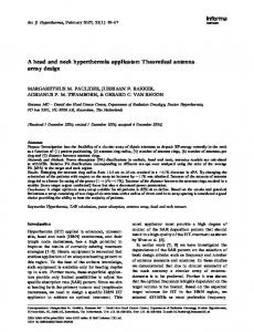
Fig. 1. 3-dimensional probe placement with 4 masks and S = ACT G. Total border length is 24 (7 on the A mask, 4 on the C mask, 6 on the T mask, and 7 on the G mask).

uncertainty, one can exploit the freedom available in assigning probes to array sites during placement and in choosing among multiple probe embeddings, when available. The objective of probe placement and embedding algorithms is therefore to minimize the sum of border lengths in all masks, which directly corresponds to the magnitude of the unintended illumination effects. 2 Reducing these effects improves the signal to noise ratio in image analysis after hybridization, and thus permits smaller array sites or more probes per array [31].3 Let M1 , M2 , . . . , MK denote the sequence of masks used in the synthesis of an array, and let ei ∈ {A,C, T, G} be the nucleotide synthesized after exposing mask Mi . Every probe in the array must be a subsequence of the nucleotide deposition sequence S = e 1 e2 . . . eK . In case a probe corresponds to multiple subsequences of S, one such subsequence, or “embedding” of the probe into S, must be chosen as the synthesis schedule for the probe. Clearly, the geometry of the masks is uniquely determined by the placement of the probes on the array and the particular synthesis schedule used for each probe. Formally, the border minimization problem is equivalent to finding a three-dimensional placement of the probes [34]: two dimensions represent the site array, and the third dimension represents the nucleotide deposition sequence S (see Figure 1). Each layer in the third dimension corresponds 2 Compared

to VLSI physical design, where multiple design metrics (including area, wirelength, timing, power consumption,

etc.) must be optimized simultaneously, DNA array physical design is simpler in that it must optimize a single objective, namely total border length. 3 Unfortunately, the lack of publicly available information about DNA array manufacturing yield makes it impossible to assign a concrete economic value to decreases in total border length.

8

to a mask that induces deposition of a particular nucleotide (A, C, G, or T ); a probe is embedded within a “column” of this three-dimensional placement representation. Border length of a given mask is computed as the number of conflicts, i.e., pairs of adjacent exposed and masked sites in the mask. Given two adjacent embedded probes p and p0 , the conflict distance d(p, p0 ) is the number of conflicts between the corresponding columns. The total border length of a three-dimensional placement is the sum of conflict distances between adjacent probes, and the border minimization problem (BMP) seeks to minimize this quantity. A special case is that of a synchronous synthesis regime, in which the nucleotide deposition sequence S is periodic, and the kth period (ACGT ) of S is used to synthesize a single (the kth ) additional nucleotide in each probe. Since in this case the embedding of a probe is predefined, the problem reduces to finding a two-dimensional placement of the probes. The border-length contribution from two probes p and p0 placed next to each other (in the synchronous synthesis regime) is simply twice the Hamming distance between them, i.e., twice the number of positions in which they differ. D.1 Previous Work on Border Length Minimization The border minimization problem was first considered for uniform arrays (i.e., arrays containing all possible probes of a given length) by Feldman and Pevzner [20], who proposed an optimal solution based on 2-dimensional Gray codes. Hannenhalli et al. [26] gave heuristics for the special case of synchronous synthesis. Their method is to order the probes in a traveling salesman problem (TSP) tour that heuristically minimizes the total Hamming distance between neighboring probes. The tour is then threaded into the two-dimensional array of sites, using a technique similar to one previously used in VLSI design [40]. For the same synchronous context, [34] suggested an epitaxial, or “seeded crystal growth”, placement heuristic similar to heuristics explored in the VLSI circuit placement literature by [43], [48]. Very recently, [35], [38] proposed methods with near-linear runtime combining simple ordering-based heuristics for initial placement, such as lexicographic sorting followed by threading, with heuristics for placement improvement, such optimal reassignment of an “independent” set of probes [50] chosen from a sliding window [18], or a rowbased implementation of the epitaxial algorithm that speeds-up the computation by considering only a limited number of candidates when filling each array site.4 Previous approaches can be 4 The

work of [35], [38] also extends probe placement algorithms to handle practical concerns such as pre-placed control probes,

presence of polymorphic probes, unintended illumination between non-adjacent array sites, and position-dependent border conflict

9

Nucleotide deposition sequence S (a) A C T G

A C

T

(b) A

(c) A

G

A C

G

G

T

G

T

G

T

T

G

A C

T

G

A

T

G

A

A

G

A

Fig. 2. (a) Periodic deposition sequence. (b) Synchronous embedding of the probes AGTA and GT GA gives 6 border conflicts (indicated by arrows). (c) “As soon as possible” asynchronous embedding of the probes AGTA and GT GA gives only 2 border conflicts.

summarized as follows: 1. TSP+Threading [26]: This algorithm computes a TSP tour in the complete graph with the probes as vertices and edge costs given by pairwise Hamming distances. The tour is then threaded into the two-dimensional array of sites using the 1-threading method described in [26]. 2. Row-Epitaxial [35], [38]: An implementation of the epitaxial algorithm in [34], where the computation is sped up by (a) filling array sites in a predefined order (row by row), and (b) considering only a limited number of candidate probes when filling each array site. Unless otherwise specified, the number of candidates is bounded by 20000 in our experiments. 3. Sliding-Window Matching (SWM) [35], [38]: After an initial placement is obtained by 1threading of the probes in lexicographic order, this algorithm iteratively improves the placement by selecting an “independent” set of probes from a sliding window and then optimally re-placing them using a minimum-weight perfect matching algorithm (cf. “row-ironing” [12]). The general border minimization problem, which allows arbitrary, or asynchronous probe embeddings (see Figure 2(c)), was introduced by Kahng et al. [34]. They proposed a dynamic programming algorithm that embeds a given probe optimally with respect to fixed embeddings of the probe’s neighbors. This algorithm is used as a building block for designing several algorithms that improve a placement by re-embedding probes, but without re-placing them. An important aspect of probe re-embedding is the probe processing order of re-embedding, i.e, the order that specifies when a probe gets re-embedded. Each of the following two algorithms uses the dynamic programming algorithm in [34] for optimal re-embedding of a probe with respect to the embeddings of its weights.

10

neighbors. They only differ in the processing order of probe re-embedding. 1. Batched greedy [34]: This algorithm optimally re-embeds a probe that gives the largest decrease in conflict cost, until no further decreases are possible. To improve the runtime, the greedy choices are made in phases, in a batched manner: in each phase the gains for all probes are computed, and then a maximal set of non-adjacent probes is selected for re-embedding by traversing the probes in non-increasing order of gain. 2. Chessboard [34]: In this method, the 2-dimensional placement grid is divided into “black” and “white” locations as in the chessboard (or checkerboard) grid of Akers [3]. The sites within each set represent a maximum independent set of locations. The Chessboard algorithm alternates between optimal re-embedding of probes placed in “black” (respectively “white”) sites with respect to their neighbors (all of which are at opposite-color locations). III. PARTITION BASED P ROBE P LACEMENT In this section we propose a probe placement heuristic inspired from min-cut partitioning based placement algorithms for VLSI circuits. Recursive partitioning has been the basis of numerous successful VLSI placement algorithms [5], [12], [52] since it produces placements with acceptable wirelength within practical runtimes. The main goal of partitioning in VLSI is to divide a set of cells into two or four sets with minimum edge or hyperedge cut between these sets. The min-cut goal is typically achieved through the use of the Fiduccia-Mattheyses procedure [21], often in a multilevel framework [12]. Unfortunately, direct transfer of the recursive min-cut placement paradigm from VLSI to VLSIPS is blocked by the fact that the possible interactions between probes must be modeled by a complete graph and, furthermore, the border cost between two neighboring placed partitions can only be determined after the detailed placement step which finalizes probe placements at the border between the two partitions. In this section we describe a new centroid-based quadrisection method that applies the recursive partitioning paradigm to DNA probe placement. Assume that at a certain depth of the recursive partitioning procedure, a probe set R is to be quadrisectioned into four partitions R1 , R2 , R3 and R4 . We would like to iteratively assign each probe p ∈ R to some partition Ri such that a minimum number of conflicts will result. 5 To ap5 Observe

that VLSI partitioning seeks to maximize the number of nets contained within partitions (equivalently, minimize cut

nets) as it assigns cells to partitions. In contrast, DNA partitioning seeks to minimize the expected number of conflicts within partitions as it assigns cells to partitions, since this leads to overall conflict reduction.

Input: Partition (set of probes) R

11

Output: Probes C0 ,C1 ,C2 , C3 to be used as centroids for the 4 subpartitions Randomly select probe C0 in R Choose C1 ∈ R maximizing d(C1 ,C0 ) Choose C2 ∈ R maximizing d(C2 ,C0 ) + d(C2,C1 ) Choose C3 ∈ R maximizing d(C3 ,C0 ) + d(C3,C1 ) + d(C3,C2 ) Return (C0 ,C1 ,C2 ,C3 ) Fig. 3. The SelectCentroid() procedure for selecting the centroid probes of subpartitions. Input: Partition R and the neighboring partition Rn ; rectangular region consisting of columns cle f t to cright and rows rtop to rbottom Output: Probes in R are placed in row-epitaxial fashion Let Q = R ∪ Rn For i = rtop to rbottom For j = cle f t to cright Find probe q ∈ Q such that d(q, pi−1, j ) + d(q, pi, j−1) is minimum Let pi, j = q Q = Q\q Fig. 4. The Reptx() procedure for placing a partition’s probe set within the rectangular array of sites corresponding to the partition. As explained in the accompanying text, our implementation maintains the size of Q constant at |Q| = 20000 through a borrowing heuristic.

proximately achieve this goal within practical runtimes, we propose to base the assignment on the number of conflicts between p and some representative, or centroid, probe C i ∈ Ri . In our approach, for every partition R we select four centroids, one for each of the four new (sub-)partitions. To achieve balanced partitions, we heuristically find four probes in R that have maximum total distance among themselves, then use these as the centroids. This procedure, described in Figure 3, is reminiscent of the k-center approach to clustering studied by Alpert et al. [4], and of methods used in large-scale document classification [16]. After a given maximum partitioning depth L is reached, a final detailed placement step is needed to place each partition’s probes within the partition’s corresponding region on the chip. For this step, we use the row-epitaxial algorithm of [35], [38], which for completeness of exposition is replicated in Figure 4.

12

Input: Chip size N × N; set R of DNA probes Output: Probe placement which heuristically minimizes total conflicts Let l = 0 and let L = maximum recursion depth Let Rl1,1 = R For l = 0 to L − 1 For i = 1 to 2l For j = 1 to 2l (C0 ,C1 ,C2 ,C3 ) ← SelectCentroid(Rli, j ) l+1 l+1 l+1 Rl+1 2i−1,2 j−1 ← {C0 }; R2i−1,2 j ← {C1 }; R2i,2 j−1 ← {C2 }; R2i,2 j ← {C3 }

For each probe p ∈ Rli, j \ {C0,C1 ,C2 ,C3 } Insert p into the yet-unfilled partition of Rli, j whose centroid has minimum distance to p For i = 1 to 2L For j = 1 to 2L Reptx(RLi, j , RLi, j+1 ) Fig. 5. Partitioning-based DNA probe placement heuristic.

The complete partitioning-based placement algorithm for DNA arrays is given in Figure 5. At a high level, our method resembles global-detailed approaches in the VLSI CAD literature [29], [46]. The algorithm recursively quadrisects every partition at a given level, assigning the probes so as to minimize distance to the centroids of subpartitions.6 In the innermost of the three nested for loops of Figure 5, we apply a multi-start heuristic, trying r different random probes as seed C0 and using the result that minimizes total distance to the centroids. Once the maximum level L of the recursive partitioning is attained, detailed placement is executed via the row-epitaxial algorithm. Additional details and commentary are as follows. •

Within the innermost of the three nested for loops, our implementation actually performs, and

benefits from, a dynamic update of the partition centroid whenever a probe is added into a given partition. Intuitively, this can lead to “elongated” rather than spheric clusters, but can also correct for unfortunate choices of the initial four centroids.7 •

The straightforward implementation of Reptx()-based detailed placement within a given partition 6 The

variables i and j index the row and column of a given partition within the current level’s array of partitions. of the dynamic centroid update, reflecting an efficient implementation, are as follows. The “pseudo-nucleotide” at each

7 Details

position t (e.g., t = 1, . . . , 25 for probes of length 25) of the centroid Ci can be represented as Ci [t] =

S Ns,t s

Ni

· s, where Ni is the current

number of probes in the partition Ri and Ns,t is the number of probes in the partition having the nucleotide s ∈ {A, T,C, G} in t-th position. The Hamming distance between a probe p and Ci is d(p,Ci ) =

1 Ni

∑ ∑ Ns,t . t s6= p[t]

13 will treat the last locations within a region “unfairly”, e.g., only one candidate probe will remain

available for placing in a region’s last location. To ensure that a uniform number of canidate probes for every position, our implementation permits “borrowing” probes from the next region in the Reptx() procedure. For every position of a region other than the last, we select the best probe from among at most m probes, where m is a pre-determined constant, in the current region and the next. (Except as noted, we set m to 20000 for all of our experiments.) Our Reptx() implementation is also “border-aware”, that is, it takes into account Hamming distances to the placed probes in adjacent regions. A. Empirical Evaluation of Partitioning-Based Probe Placement In this section we compare our partitioning-based probe placement heuristic with the TSP 1threading heuristic of [26] (TSP+1Thr), the Row-Epitaxial and sliding-window matching (SWM) heuristics of [35], and a simulated annealing algorithm (SA).8 We used an upper bound of 20000 on the number of candidate probes in Row-Epitaxial, and 6 × 6 windows with overlap 3 for SWM. The SA algorithm starts by sorting the probes and threading them onto the chip. It then slides a square window over the chip in the same way as the SWM algorithm. For every window position, SA picks 2 random probes in the window and swaps them with probability 1 if the swap improves total border cost. If the swap increases border cost by δ, the swap is performed only with probability e−δ/T , where T is the current temperature. After experimenting with various SA parameters, we chose to run SA with 6 × 6 windows with overlap of 3, with 63 iterations performed for every window position. Table I gives the results produced by the TSP+1Thr, Row-Epitaxial, SWM, and SA heuristics on random instances with chip sizes between 100 and 500 and probe length equal to 25. Among the four heuristics, Row-Epitaxial is the algorithm with highest solution quality (i.e., lowest border cost), while SWM is the fastest, offering competitive solution quality with much less runtime. SA takes the largest amount of time, and also gives the worse solution quality. Although it may be possible to improve SA convergence speed by extensive fine-tuning of its various parameters, we expect that SA results will always remain dominated by those of the other heuristics. Additional 8 All

experiments reported in this paper were performed on test cases obtained by generating each probe candidate uniformly at

random. The probe length was set to 25, which is the typical value for commercial arrays [1]. Unless otherwise noted, we used the canonical periodic deposition sequence, (ACT G)25 . All reported runtimes are for a 2.4 GHz Intel Xeon server with 2GB of RAM running under Linux.

14

insight into the relative quality of various heuristics can be gained by considering the border cost normalized by the number of pairs of adjacent array sites, i.e., the average number of conflicts per pair of adjacent sites. Interestingly, for all algorithms except SA this number decreases with increasing chip size. This can be attributed to the greater freedom of choice available when placing a higher number of probes, which all algorithms except SA seem able to exploit. Tables II and II give results obtained by our new recursive partitioning method (RPART) with recursion depth L = 2 and number of restarts r varying between 1 and 1000. The results in Tables II show that increasing the number of restarts gives a small improvement in border cost at the expense of increased runtime. Table III presents results obtained by RPART when run with r = 10 for recursion depth L varying between 1 and 3. Comparing to the results produced by Row-Epitaxial, the best heuristic from Table I, we find that recursive partitioning based placement achieves on the average similar or better results with improved runtime. We next discuss in more detail the runtime of RPART, which is somehow unusual for a recursive partitioning algorithm in that it may get smaller with an increase in recursion depth. Let the number of probes in a chip be n. The two main contributors to RPART runtime are the recursive partioning phase, whereby the probes are divided into smaller and smaller partition regions, and the detailed placement step which is achieved by running Row-Epitaxial within each partition region (with borrowing from next region when needed). Since executing the procedure SelectCentroid() and distributing all the probes in a partition region to its four sub-regions takes time proportional to the number of probes in a region, the total runtime for each recursion depth is O(n), and the overall runtime for the recursive partitioning phase is O(Ln). Clearly, this component of the runtime increases linearly with the recursion depth. On the other hand, in our implementation of RPART, the Row-Epitaxial algorithm used in detailed placement considers at most min{m, 2n/4 L} candidate probes for placement at any given position (m = 20000 is a pre-determined upper-bound which we impose based on the empirical results in [35], and 2n/4 L is a bound that follows from the fact that we never consider candidates from more than two consecutive lowest-level partition regions). Thus, the total time needed by the detailed placement step is O(n min{m, 2n/4 L }), which will decrease with increasing L once L exceeds log4 (2n/m). This explains why the overall RPART runtime in Table III decreases with increasing L, and also explains why solution quality may slightly degrade with increasing L due to the reduced number of probe candidates considered by Row-Epitaxial for each chip location.

Chip Lower Bound Size

TSP+1Thr

Cost Norm.

Row-Epitaxial

Cost Norm. Gap(%)

CPU 113

15 SA

SWM

Cost Norm. Gap(%) CPU 108

Cost Norm. Gap(%) CPU

Cost Norm. Gap(%)

CPU

100 410019

20.7

554849

28.0

35.3

200 1512014

19.0 2140903

26.9

41.6

502314

25.4

22.5

605497

30.6

47.7

2

583926

29.8 42.4% 20769

1901 1913796

24.0

26.6 1151 2360540

29.7

56.1

8 2418372

30.4 59.9% 55658

300 3233861

18.0 4667882

26.0

44.3 12028 4184018

24.0

29.4 3671 5192839

28.9

60.6

19 5502544

30.7 70.2% 103668

500 8459958

17.0 12702474

25.5

50.1 109648 11182346

22.4

32.2 10630 13748334

27.6

62.5

50 15427304

30.9 82.5% 212390

TABLE I T OTAL BORDER LOWER - BOUND IN HEURISTIC OF

COST, NORMALIZED BORDER COST, GAP FROM THE SYNCHRONOUS PLACEMENT

[34], AND CPU

[26] (TSP+1T HR ),

(SWM)

Size 100

THE ROW- EPITAXIAL

HEURISTICS OF

Chip RPART r = 1 L = 2

24.9

[35], AND

10 RANDOM

INSTANCES ) FOR THE

(ROW-E PITAXIAL ) AND

TSP

SLIDING - WINDOW MATCHING

THE SIMULATED ANNEALING ALGORITHM

(SA).

RPART r = 10 L = 2 RPART r = 100 L = 2 RPART r = 1000 L = 2

Cost Norm. CPU 492054

SECONDS ( AVERAGES OVER

22

Cost Norm. CPU 491840

24.8

24

Cost Norm. CPU 491496

24.8

Cost Norm. CPU

47

490809

24.8

238

200 1865972

23.4 276 1865337

23.4 283 1864982

23.4

394 1864017

23.4 1064

300 4075214

22.7 1501 4074962

22.7 1527 4073135

22.7 1769 4071344

22.7 4231

500 11063382

22.2 9531 11052738

22.1 9678 11042812

22.1 13158 11039731

22.1 17014

TABLE II T OTAL / NORMALIZED BORDER

COST AND

CPU

SECONDS ( AVERAGES OVER

RECURSIVE PARTITIONING ALGORITHM WITH RECURSION DEPTH FROM

1

TO

10 RANDOM

L = 2 AND

INSTANCES ) FOR THE

NUMBER OF RESTARTS

r

VARYING

1000.

Chip Lower Bound

RPART r = 10 L = 1

RPART r = 10 L = 2

RPART r = 10 L = 3

Size

Cost Norm. Gap(%) CPU

Cost Norm. Gap(%) CPU

Cost Norm. Gap(%) CPU

Cost Norm.

100 410019

20.7

475990

24.0

16.1

200 1512014

19.0 1813105

22.8

19.9

300 3233861

18.0 4135728

500 8459958

17.0 11283631

69

491840

24.8

20.0

24

504579

25.5

23.1

10

992 1865337

23.4

23.4 283 1922951

24.2

27.2

81

23.8

27.9 3529 4074962

22.7

26.0 1527 4175146

24.0

29.1 240

22.6

33.4 10591 11052738

22.1

30.6 9678 11134960

22.3

31.6 3321

TABLE III T OTAL BORDER LOWER - BOUND IN

COST, NORMALIZED BORDER COST, GAP FROM THE SYNCHRONOUS PLACEMENT

[34], AND CPU

SECONDS ( AVERAGES OVER

10 RANDOM

INSTANCES ) FOR THE RECURSIVE

PARTITIONING ALGORITHM WITH RECURSION DEPTH VARYING BETWEEN

1 AND 3.

16

Chip Lower Bound Size

Batched Greedy

Cost Norm.

Chessboard

Cost Norm. Gap(%) CPU 40

Sequential

Cost Norm. Gap(%) CPU 54

Cost Norm. Gap(%) CPU

100 364953

18.4

458746

23.2

25.7

439768

22.2

20.5

437536

22.1

19.9

64

200 1425784

17.9 1800765

22.6

26.3 154 1723773

21.7

20.9 221 1715275

21.5

20.3 266

300 3130158

17.4 3965910

22.1

26.7 357 3803142

21.2

21.5 522 3773730

21.0

20.6 577

500 8590793

17.2 10918898

21.9

27.1 943 10429223

20.9

21.4 1423 10382620

20.8

20.9 1535

TABLE IV T OTAL BORDER LOWER - BOUND IN

COST, NORMALIZED BORDER COST, GAP FROM THE ASYNCHRONOUS POST- PLACEMENT

[34], AND CPU

SECONDS ( AVERAGES OVER

10 RANDOM

INSTANCES ) FOR THE BATCHED

GREEDY, CHESSBOARD , AND SEQUENTIAL IN - PLACE RE - EMBEDDING ALGORITHMS .

B. Comparison of Complete Probe Placement and Embedding Flows In addition to the partitioning-based placement algorithm, we propose a new algorithm that performs optimal re-embedding of probes in a sequential row-by-row fashion. We believe that a main shortcoming of Batched Greedy and Chessboard (described in Section II-D.1) is that these methods always re-embed an independent set of sites on the DNA chip. Dropping this requirement permits faster propagation of the effects of any re-embedding decision. Table IV compares the new probe embedding algorithm with Batched Greedy and Chessboard on random instances with chip sizes between 100 and 500 and probe length 25 for which the twodimensional placements were obtained using TSP+1-threading. All algorithms are stopped when the improvement cost achieved in one iteration over the whole chip drops below 0.1% of the total cost. The results show that re-embedding of the probes in a sequential row-by-row order leads to reduced border cost with similar runtime compared to previous methods. In another series of experiments, we ran complete placement and embedding flows obtained by combining each of the five two-dimensional placement algorithms evaluated in Section III-A with the sequential in-place re-embedding algorithm. Results are given in Tables V-VI. Again, SA and TSP+1Thr are dominated by both REPTX and SWM in both conflict cost and running time. REPTX produces less conflicts than SWM but SWM is considerably faster. Recursive partitioning consistently outperforms the best previous flow (row-epitaxial + sequential re-embedding) – by an average of 4.0% – with similar or lower runtime.

Chip Lower Bound Size

TSP+1Thr

Cost Norm.

Row-Epitaxial

Cost Norm. Gap(%)

CPU

SWM

Cost Norm. Gap(%) CPU 88.3

161

SA

Cost Norm. Gap(%) CPU 99.8

93

17

Cost Norm. Gap(%)

CPU

100 220497

11.1

439829

22.2

99.5

113 415227

21.0

440648

22.3

457752

23.1

107.6 11713

200 798708

10.0 1723352

21.7

115.8

1901 1608382

20.2

101.4 1368 1721633

21.6

115.6 380 1844344

23.2

130.9 42679

300

—

— 3801765

21.2

— 12028 3529745

20.3

— 3861 3801479

21.2

— 861 4155240

23.2

— 101253

500

—

— 10426237

20.9

— 109648 9463941

19.0

— 12044 10161979

20.4

— 2239 11574482

23.2

— 222376

TABLE V T OTAL BORDER

COST, NORMALIZED BORDER COST, GAP FROM THE ASYNCHRONOUS PRE - PLACEMENT

LOWER - BOUND IN HEURISTIC OF

[26] (TSP+1T HR ),

(SWM)

SECONDS ( AVERAGES OVER

THE ROW- EPITAXIAL

HEURISTICS OF

[35], AND

Cost Norm.

10 RANDOM

(ROW-E PITAXIAL ) AND

INSTANCES ) FOR THE

RPART r = 10 L = 2

Cost Norm. Gap(%) CPU

TSP

SLIDING - WINDOW MATCHING

THE SIMULATED ANNEALING ALGORITHM

RPART r = 10 L = 1

Chip Lower Bound Size

[34], AND CPU

(SA).

RPART r = 10 L = 3

Cost Norm. Gap(%) CPU

Cost Norm. Gap(%) CPU

100 220497

11.1 393218

19.9

78.3

123 399312

20.2

81.1

44 410608

20.7

86.2

200 798708

10.0 1524803

19.2

90.9 1204 1545825

19.4

93.5

365 1573096

19.8

97.0 101

300

—

— 3493552

20.1

— 3742 3413316

19.6

— 1951 3434964

19.7

— 527

500

—

— 9546351

19.1

— 11236 9355231

18.8

— 10417 9307510

18.7

— 3689

10

TABLE VI T OTAL BORDER LOWER - BOUND IN

COST, NORMALIZED BORDER COST, GAP FROM THE ASYNCHRONOUS PRE - PLACEMENT

[34], AND CPU

SECONDS ( AVERAGES OVER

10 RANDOM

INSTANCES ) FOR THE RECURSIVE

PARTITIONING ALGORITHM FOLLOWED BY SEQUENTIAL IN - PLACE RE - EMBEDDING .

IV. F LOW E NHANCEMENTS The current DNA-array design flow can be significantly improved by introducing flow-aware problem formulations, adding feedback loops between optimization steps, and/or integrating multiple optimizations. These enhancements, which are represented schematically in Figure 6 by the dashed arcs, are similar to flow enhancements that have proved very effective in the VLSI design context [19], [49]. In this paper we concentrate on two such enhancements, both aiming at further reductions in total border length. The first enhancement is a tighter integration between probe placement and embedding; this enhancement is discussed in Section IV-B. The second enhancement is the inte-

18

Probe pools

Probe Selection

Deposition Sequence Design

Test Structure Design

Physical Design Probe placement

Probe Embedding

Fig. 6. A typical DNA array design flow with solid arcs and proposed enhancements represented by dashed arcs.

gration between physical design and probe selection, which is achieved by passing the entire pools of candidates available for each probe to the physical design step. As shown in Section IV-C, this enhancement enables significant improvements (up to 15%) in border length compared to best previous flows [35], [38]. Other feedback loops and integrated optimizations are possible but are not explored in this paper. Faster and more targeted probe selection may be achievable by adding a feedback loop to provide updated selection rules and parameters to the probe selection step. Integrating deposition sequence design with probe selection may lead to further reductions in the number of masks by exploiting the freedom available in choosing the candidates for each probe. A. Problem Formulation for Integrated Probe Selection and Physical Design To integrate probe selection and physical design, we pass the entire pools of candidates for each probe to the physical design step (Figure 6). As discussed in Section II-A, all probe candidates are selected so that they have similar hybridization properties (e.g., melting temperatures), and can thus be used interchangeably. The availability of multiple probe candidates gives additional freedom during placement and embedding, and may potentially reduce final border cost. DNA array physical design with probe pools is captured by the following problem formulation: 9 Integrated DNA Array Design Problem Given: •

Pools of candidates Pi = {pi j | j = 1, . . ., li } for each probe i = 1, . . . , N 2 , where N × N is the size

of array •

The number of masks K

Find: 1. Probes pi j ∈ Pi for every i = 1, . . . , N 2 , 9 This

formulation also integrates deposition sequence design. For simplicity, we leave out design of control and test sequences.

2. A deposition sequence S = s1 , . . ., sK which is a supersequence of all selected probes pi j ,

19

3. A placement of the selected probes pi j into an N × N array, 4. An embedding of the selected probes pi j into the deposition sequence S Such that: •

The total number of conflicts between adjacent embedded probes is minimized Although the flow in Figure 6 suggests a particular order for making the choices 1-4, the inte-

grated formulation above allows interleaving these decisions. The following two algorithms capture key optimizations in the integrated formulations, and are used as core building blocks in the solution methods evaluated in Sections IV-B–IV-C. They are “probe pool” versions of the Rowepitaxial and re-embedding algorithms proposed in [35], [38], and degenerate to the latter ones in the case when each probe pool contains a single candidate. •

The Pool Row-Epitaxial algorithm (Pool-REPTX) is the extension to probe pools of the REPTX

probe placement algorithm in [35], [38]. Pool-REPTX performs choices 1 and 3 for given choices 2 and 4, i.e., it simultaneously chooses already embedded candidates from the respective pools and places them in the N × N array. The input of Pool-REPTX consists of probe candidates p i j embedded in the deposition sequence S. Each such embedding is written as a sequence of length K = |S| over the alphabet {A,C, T, G, Blank}, where A,C, T, G denote embedded nucleotides and Blank’s denote positions of S left unused by the embedded candidate probe. Pool-REPTX consists of the following steps: (1) Lexicographic sorting of the pools (based on the first candidate, when more than one candidate is available in the pool); (2) Threading the sorted pools in row-by-row order into the N × N array; (3) Finding, in row-by-row order, the best probe candidate – i.e., the candidate having the minimum number of conflicts with already placed neighbors – among the not yet placed pools within a prescribed lookahead region. •

The sequential in-place pool re-embedding algorithm is the extension to probe pools of the se-

quential probe re-embedding algorithm given in Section III-B. It complements Pool-REPTX by iteratively modifying candidate selections within each pool and their embedding (choices 2 and 4) as follows. In row-by-row order, for each position in the N × N array, and for each candidate p i j from the pool of the respective probe, an embedding having minimum number of conflicts with the existing embeddings of the neighbors is computed, and then the best embedded candidate replaces the current one.

20

B. Improved Integration of Probe Placement and Embedding As noted in [34], allowing arbitrary, or asynchronous, embeddings leads to further reductions in border length compared to synchronous embedding (e.g., contrast (b) and (c) in Figure 2). An interesting question is finding the best order in which the placement and embedding degrees of freedom should be exploited. Previous methods [34], [35], [38] can be divided into two classes: (1) methods that perform placement and embedding decisions simultaneously, and (2) methods that exploit the two degrees of freedom one at a time. Currently, best methods in the second class (e.g., synchronous row-epitaxial followed by chessboard/sequential in-place probe re-embedding [35], [38]) outperform the methods in the first class (e.g., the asynchronous epitaxial algorithm in [34]) in terms of both runtime and solution quality. All known methods in the second class perform synchronous probe placement followed by iterated in-place re-embedding of the probes (with locked probe locations). More specifically, these methods perform the following 3 steps: •

Synchronous embedding of the probes.

•

Probe placement with costs given by the Hamming distance between the synchronous probe

embeddings. •

Iterated sequential probe re-embedding.

We note that significant reductions in border cost are possible by performing the placement based on asynchronous, rather than synchronous, embeddings of the probes, and therefore modify the above scheme as follows: •

Asynchronous embedding of the probes.

•

Placement with costs given by the Hamming distance between the fixed asynchronous probe

embeddings. •

Iterated sequential probe re-embedding. Since solution spaces for placement and embedding are still searched independently of one an-

other, and the computation of an initial asynchronous embedding does not add significant overhead, the proposed change is unlikely to adversely affect the runtime. However, because placement optimization is now applied to embeddings more similar to those sought in the final optimization stage, there is significant potential for improvement. In the current embodiment of the modified scheme, we implement the first step by using for each probe the “as soon as possible,” or ASAP, embedding (see Figure 2(c)). Under ASAP embedding

Chip

Synchronous Initial Embedding

ASAP Initial Embedding

Percent

Sync Embed

REPTX

Re-Embed

ASAP Embed

REPTX

Re-Embed

Improv.

100

619153

502314

415227

514053

393765

389637

5.2

200

2382044

1918785

1603745

1980913

1496937

1484252

6.7

300

5822857

4193439

3514087

4357395

3273357

3245906

6.9

500

18786229

11203933

9417723

11724292

8760836

8687596

7.0

21

TABLE VII T OTAL BORDER

COST ( AVERAGES OVER

10 RANDOM

INSTANCES ) FOR SYNCHRONOUS AND

ASAP

INITIAL

PROBE EMBEDDING FOLLOWED BY ROW- EPITAXIAL AND ITERATED SEQUENTIAL IN - PLACE PROBE RE - EMBEDDING .

the nucleotides in a probe are embedded sequentially by always using the earliest available synthesis step. The intuition behind using ASAP embeddings is that, since ASAP embeddings are more densely packed, the likelihood that two neighboring probes will both use a synthesis step increases compared to synchronous embeddings. This translates directly into reductions in the number of border conflicts. Indeed, consider two random probes p, p0 picked from the uniform distribution. When we perform synchronous embedding, the length of the deposition sequence is 4 × 25 = 100. The probability that any one of the 100 synthesis step is used by one of the random probes and not the other is 2 × (1/4) × (3/4), and therefore the expected number of conflicts is 100 × 2 × (1/4) × (3/4) = 37.5. Assume now that the two probes are embedded using the ASAP algorithm. Notice that for every 0 ≤ i ≤ 3 the ASAP algorithm will leave a gap of length i with probability 1/4 between any two consecutive letters of a random probe. This results in an average gap length of 1.5, and an expected number of synthesis steps of 25 + 24*1.5 = 61. Assuming that p and p 0 are both embedded within 61 steps, the number of conflicts between their ASAP embeddings is then approximately 61 × 2 × (25/61) × ((61 − 25)/61) ≈ 29.5. Although in practice many probes require more than 61 synthesis steps when embedded using the ASAP algorithm, they still require much less than 100 steps and result in significantly fewer conflicts compared to synchronous embedding. To empirically evaluate the advantages of ASAP embedding we compared on test cases ranging in size from 100 × 100 to 500 × 500 the “champion” method in [34], [35], [38], which uses synchronous initial embeddings for the probes, with the corresponding method based on ASAP initial

22

Chip

Synchronous Initial Embedding

ASAP Initial Embedding

Sync+REPTX

Re-Embed

Total

ASAP+REPTX

Re-Embed

Total

100

166

81

247

188

29

217

200

1227

340

1567

1302

114

1416

300

3187

748

3935

2736

235

2971

500

8495

2034

10529

6391

451

6842

TABLE VIII CPU

SECONDS ( AVERAGES OVER

10 RANDOM

INSTANCES ) FOR SYNCHRONOUS AND

ASAP

INITIAL PROBE

EMBEDDING FOLLOWED BY ROW- EPITAXIAL AND ITERATED SEQUENTIAL IN - PLACE PROBE RE - EMBEDDING .

probe embeddings. For both methods, the second and third steps are implemented using REPTX and sequential in-place probe re-embedding algorithms in [35], [38] (see also Section IV-A). Tables VII and VIII give the border-length and CPU time (in seconds) for the two methods. Each number in these tables represents the average over 10 test cases of the given size. Surprisingly, the simple switch from synchronous to ASAP initial embedding results in 5-7% reduction in total border-length. Furthermore, the runtimes for the two methods are comparable. In fact, sequential re-embedding becomes faster in the ASAP-based method compared to the synchronous-based one since fewer iterations are needed to converge to a locally optimal solution (the number of iterations drops from 9 to 3 on the average). C. Integrated Probe Selection and Physical Design We explored two methods for exploiting the availability of multiple probe candidates during placement and embedding. The first method uses the row-epitaxial and sequential in-place probe re-embedding algorithms described in Section IV-A. This method is an instance of integration between multiple flow steps, since probe selection decisions are made during probe placement and can be further changed during probe re-embedding. The detailed steps are as follows: •

Perform ASAP embedding of all probe candidates.

•

Run the Pool-REPTX or a pool version of the recursive-partitioning placement algorithm in

Section III using border costs given by the Hamming distance between the ASAP embeddings. •

Run the sequential in-place pool re-embedding algorithm. The second method preserves the separation between candidate selection and place-

ment+embedding. However, we modify probe selection to make it flow-aware, i.e., to make its

23 results more suitable for the subsequent placement and embedding optimizations. Building on

the observation that shorter probe embeddings lead to improved border length, we choose from the available candidates the one that embeds in the least number of steps of the standard periodic deposition sequence using ASAP: •

Perform ASAP embedding of all probe candidates.

•

Select from each pool of candidates the one that embeds in the least number of steps using ASAP.

•

Run the REPTX or recursive-partitioning placement algorithm using only the selected candidates

and border costs given by the Hamming distance between the ASAP embeddings. •

Run the iterated sequential in-place probe re-embedding algorithm, again using only selected

candidates. Table IX gives the border-length and the runtime (in CPU seconds) for the two methods of combining probe placement and embedding with probe selection (each number represents the average over 10 test cases of the given size). We report results for both Pool-REPTX placement algorithm and the pool version of the recursive-partitioning using L = 3. We varied the number of candidates available for each probe between 1 and 16; probe candidates were generated uniformly at random. As expected, for each method and chip size, the improvement in solution quality grows monotonically with the number of available candidates. The improvement is significant (up to 15% when running the first method on a 100×100 chip with 16 candidates per probe), but varies nonuniformly with the method and chip size. For small chips the first method gives better solution quality than the second. For chips of size 200×200 the two methods give comparable solution quality, while for chips with size 300×300 or larger the second method is better (by over 5% for 500×500 chips with 8 probe candidates). The second method is faster than first for all chip sizes. The speedup factor varies between 5× and 40× when the number of candidates varies between 2 and 16. Interestingly, the runtime of the second method is slightly improving with the number of candidates, the reason being that the number of iterations of sequential re-embedding decreases when the length of the ASAP embedding of the selected candidates decreases. V. Q UANTIFIED

SUB - OPTIMALITY OF PLACEMENT AND EMBEDDING ALGORITHMS

As noted in the introduction, next-generation of DNA probe arrays will contain up to one hundred million probes, and therefore present instance complexities for placement that will far outstrip those of VLSI designs. Thus, it is of interest to study not only runtime scaling, but also scaling

24

of suboptimality, for available heuristics. To this end, we apply the experimental framework for quantifying suboptimality of placement heuristics that was originated by Boese and by Hagen et al. [27], and recently extended by Chang et al. [13] and Cong et al. [15]. In this framework, there are two basic types of instance scaling that we can apply. •

Instances with known optimum solution.

For hypergraph placement, instances with known

minimum-wirelength solutions may be constructed by “overlaying” signal nets within an already placed cell layout, such that each signal net has provably minimum length. This technique, proposed by Boese and further explored by Chang et al. [13], induces a netlist topology with prescribed degree sequence over the (placed) cells; this corresponds to a “placement example with known optimal wirelength” (PEKO). In our DNA probe placement context, there is no need to generate a netlist hypergraph. Rather, we realize the concept of minimum (border) cost edges (adjacencies) by constructing a set of probes, and their placement, using 2-dimensional Gray codes [20]. Our construction generates 4k probes which are placeable such that every probe has border cost of 2 to each of its neighboring probes. This construction is illustrated in Figure 7. •

Instances with known suboptimal solutions.

Because constructed instances with known op-

timum solutions may not be representative of “real” instances, we also apply a technique [27] that allows real instances to be scaled, such that they offer insights into scaling of heuristic suboptimality. The technique is applied as follows. Beginning with a problem instance I, we construct three isomorphic versions of I by three distinct mappings of the nucleotide set {A,C, G, T } onto itself. Each mapping yields a new probe set that can be placed with optimum border cost exactly equal to the optimum border cost of I. Our scaled instance I 0 consists of the union of the original probe set and its three isomorphic copies. Observe that one placement solution for I 0 is to optimally place I and its isomorphic copies as individual chips, and then to adjoin these placements as the four quadrants of a larger chip. Thus, an upper bound on the optimum border cost for I 0 is 4 times the optimum border cost for I, plus the border cost between the copies of I; see Figure 8. If a heuristic H places I 0 with cost cH (I 0 ) ≥ 4 · cH (I), then we may infer that the heuristic’s suboptimality is growing by at least a factor

cH (I 0 ) 4·cH (I) .

On the other hand, if cH (I 0) < 4 · cH (I), then the heuristic’s

solution quality would be said to scale well on this class of instances. Table X shows results from executing the various placement heuristics on PEKO-style test cases, with instance sizes ranging from 16 x 16 through 512 x 512 (recall that our Gray code construction yields instances with 4k probes). We see from these results that sliding-window matching is closest

AM11

AM1n TM1n

TM11

25

M 1n

M 11

M n1

AMn1

AMnn TMnn

TMn1

CM n1

CMnn GMnn

GMn1

CM11

CMn1 GMn1

GM11

M nn n=2

t

Fig. 7. 2-dimensional Gray code placement. (A, T, C, G) −−> (C, G, A, T)

(A, T, C, G) −−> (A, T, C, G)

A

C

A

T

C

G

T

C

G

A

C

G







 
 

T A G

T A

G

(A, T, C, G) −−> (T, C, G, A)



 

T

C

(A, T, C, G) −−> (G, A, T, C)

Fig. 8. Scaling construction used in the suboptimality experiment.

to the optimum, with a suboptimality gap of 4-30%. Overall, DNA array placement algorithms appear to be performing better than their VLSI counterparts [13] when it comes to results on special-case instances with known optimal cost. Of course, results from placement algorithms (whether for VLSI or DNA chips) on special benchmark instances should not be generalized to arbitrary benchmarks. In particular, our results show that algorithms that perform best for arbitrary benchmarks are not necessarily the best performers for specially constructed benchmarks. Table XI shows results from executing the various placement heuristics on scaled versions of random DNA probe sets, with the original instances ranging in size from 100 x 100 to 500 x 500, and the scaled instances thus ranging in size from 200 x 200 to 1000 x 1000. This table shows that in general, placement algorithms for DNA arrays offer excellent scaling suboptimality. We believe that this is primarily due to the already noted fact that algorithm quality (as reflected by normalized border costs) improves with instance size. The larger number of probes in the scaled instances gives more freedom to the placement algorithms, leading to heuristic placements that have scaling suboptimality factor well below 1.

26

VI. C ONCLUSIONS In this work, we have studied several problems arising in the design of DNA chips, focusing

on minimizing the total border length between adjacent sites during probe placement and embedding. We have shown that significant reductions in border length can be obtained by drawing on algorithmic techniques developed in the field of VLSI design automation. We conclude with some remarks on the similarities and differences between VLSI physical design and physical design for DNA arrays. First, while VLSI placement performance in general degrades as the problem size increases, it appears that this is not the case for DNA array placement. Current algorithms are able to find DNA array placements with smaller normalized border cost when the number of probes in the design grows. Second, the lower bounds for DNA probe placement and embedding appear to be tighter than those available in the VLSI placement literature. Developing even tighter lower bounds is, of course, an important open problem. Other direction of future research is to find formulations and methods for integrated optimization of test structure design and physical design. Since test structures are typically pre-placed at sites uniformly distributed across the array, integrated optimization can have a significant impact on the total border length. R EFERENCES [1]

http://www.affymetrix.com

[2]

http://www.perlegen.com

[3]

S. Akers, “On the Use of the Linear Assignment Algorithm in Module Placement,” Proc. 1981 ACM/IEEE Design Automation Conference (DAC’81), pp. 137–144.

[4]

C. J. Alpert and A. B. Kahng, “Geometric Embeddings for Faster (and Better) Multi-Way Netlist Partitioning” Proc. ACM/IEEE Design Automation Conf., 1993, pp. 743-748.

[5]

C.J. Alpert and A.B. Kahng, “Recent directions in netlist partitioning: A survey”, Integration: The VLSI Jour. 19 (1995), pp.

[6]

N. Alon, C. J. Colbourn, A. C. H. Lingi and M. Tompa, “Equireplicate Balanced Binary Codes for Oligo Arrays”, SIAM

1-81. Journal on Discrete Mathematics 14(4) (2001), pp. 481-497. [7]

A.A. Antipova, P. Tamayo1 and T.R. Golub, “ A strategy for oligonucleotide microarray probe reduction”, Genome Biology 2002 3(12):research0073.1-0073.4

[8]

M. Atlas, N. Hundewale, L. Perelygina and A. Zelikovsky, “Consolidating Software Tools for DNA Microarray Design and Manufacturing”, Proc. International Conf. of the IEEE Engineering in Medicine and Biology (EMBC’04), 2004, pp. 172-175.

[9]

K. Nandan Babu and S. Saxena, “Parallel algorithms for the longest common subsequence problem”, Proc. 4th Intl. Conf. on High-Performance Computing, Dec. 1997, pp. 120-125.

[10] J. Branke and M. Middendorf, “Searching for shortest common supersequences”, Proc. Second Nordic Workshop on Genetic Algorithms and Their Applications, 1996, pp. 105-113.

27

[11] J. Branke, M. Middendorf and F. Schneider, “Improved heuristics and a genetic algorithm for finding short supersequences”, OR Spektrum 20(1) (1998), pp. 39-46. [12] A. Caldwell and A. Kahng and I. Markov, “Can Recursive bisection Produce Routable Designs?”, DAC, 2000, pp.477-482. [13] C. C. Chang, J. Cong and M. Xie, “Optimality and Scalability Study of Existing Placement Algorithms”, Proc. Asia SouthPacific Design Automation Conference, Jan. 2003. [14] C.J. Colbourn, A.C.H. Lingi and M. Tompa, “Construction of optimal quality control for oligo arrays”, Bioinformatics 18(4) (2002), pp. 529–535. [15] J. Cong, M. Romesis and M. Xie, “Optimality, Scalability and Stability Study of Parititoning and Placement Algorithms”, Proc. ISPD, 2003, pp. 88-94. [16] D. R. Cutting, D. R. Karger, J. O. Pederson and J. W. Tukey, “Scatter/Gather: A Cluster-Based Approach to Browsing Large

Document Collections”, (15th Intl. ACM/SIGIR Conference on Research and Development in Information Retrieval) SIGIR Forum (1992), pp. 318–329. [17] V. Dancik, “Common subsequences and supersequences and their expected length”, Combinatorics, Probability and Computing 7(4) (1998), pp. 365-373. [18] K. Doll, F. M. Johannes, K. J. Antreich, “Iterative Placement Improvement by Network Flow Methods”, IEEE Transactions on Computer-Aided Design 13(10) (1994), pp. 1189-1200. [19] J. J. Engel et al. ”Design methodology for IBM ASIC products”, IBM Journal for Research and Development 40(4) (1996), pp. 387. [20] W. Feldman and P.A. Pevzner, “Gray code masks for sequencing by hybridization”, Genomics, 23 (1994), pp. 233–235. [21] C. M. Fiduccia and R. M. Mattheyses, “A Linear-Time Heuristic for Improving Network Partitions”, Proc. Design Automation Conference (DAC 1982), pp. 175–181. [22] S. Fodor, J. L. Read, M. C. Pirrung, L. Stryer, L. A. Tsai and D. Solas, “Light-Directed, Spatially Addressable Parallel Chemical Synthesis”, Science 251 (1991), pp. 767–773. [23] D. E. Foulser, M. Li and Q. Yang, “Theory and algorithms for plan merging”, Artificial Intelligence 57(2-3) (1992), pp. 143-181. [24] C. B. Fraser and R. W. Irving, “Approximation algorithms for the shortest common supersequence”, Nordic J. Computing 2 (1995), pp. 303-325. [25] D.H. Geschwind and J.P. Gregg (Eds.), Microarrays for the neurosciences: an essential guide, MIT Press, Cambridge, MA, 2002. [26] S. Hannenhalli, E. Hubbell, R. Lipshutz and P. A. Pevzner, “Combinatorial Algorithms for Design of DNA Arrays,” in Chip Technology (ed. J. Hoheisel), Springer-Verlag, 2002. [27] L. W. Hagen, D. J. Huang and A. B. Kahng, “Quantified Suboptimality of VLSI Layout Heuristics”, Proc. ACM/IEEE Design Automation Conf., 1995, pp. 216–221. [28] S. A. Heath and F. P. Preparata, “Enhanced Sequence Reconstruction With DNA Microarray Application”, Proc. 2001 Annual International Conf. on Computing and Combinatorics (COCOON’01), pp. 64-74. [29] D. J. Huang and A. B. Kahng, “Partitioning-Based Standard-Cell Global Placement with an Exact Objective”, in Proc. ACM/IEEE Intl. Symp. on Physical Design, Napa, April 1997, pp. 18-25. [30] E. Hubbell and P.A. Pevzner, “Fidelity Probes for DNA Arrays”, Proc. Seventh International Conference on Intelligent Systems for Molecular Biology, 1999, pp. 113-117. [31] E. Hubbell and M. Mittman , personal communication (Affymetrix, Santa Clara, CA), July 2002. [32] T. Jiang and M. Li, “On the approximation of shortest common supersequences and longest common subsequences”, SIAM J. on Discrete Mathematics 24(5) (1995), pp. 1122-1139.

28

[33] L. Kaderali and A. Schliep, “Selecting signature oligonucleotides to identify organisms using DNA arrays”, Bioiformatics 18:1340-1349, 2002. [34] A.B. Kahng, I.I. M˘andoiu, P.A. Pevzner, S. Reda, and A. Zelikovsky, “Border Length Minimization in DNA Array Design”, Proc. 2nd International Workshop on Algorithms in Bioinformatics (WABI 2002), R. Guig´o and D. Gusfield (Eds.), SpringerVerlag Lecture Notes in Computer Science Series 2452, pp. 435-448. [35] A.B. Kahng, I.I. M˘andoiu, P.A. Pevzner, S. Reda, and A. Zelikovsky, “Engineering a Scalable Placement Heuristic for DNA Probe Arrays”, Proc. 7th Annual International Conference on Research in Computational Molecular Biology (RECOMB 2003), W. miller, M. Vingron, S. Istrail, P. Pevzner and M. Waterman (Eds.), 2003, pp. 148–156. [36] A.B. Kahng, I.I. M˘andoiu, S. Reda, X. Xu, and A. Zelikovsky. Design flow enhancements for DNA arrays. In Proc. IEEE International Conference on Computer Design (ICCD), pages 116–123, 2003. [37] A.B. Kahng, I.I. M˘andoiu, S. Reda, X. Xu, and A. Zelikovsky. Evaluation of placement techniques for DNA probe array layout. In Proc. IEEE-ACM International Conference on Computer-Aided Design (ICCAD), pages 262–269, 2003. [38] A.B. Kahng, I.I. M˘andoiu, P. Pevzner, S. Reda, and A. Zelikovsky. Scalable heuristics for design of DNA probe arrays. Journal of Computational Biology, 11(2–3):429–447, 2004. [39] S. Kasif, Z. Weng, A. Derti, R. Beigel, and C. DeLisi, “A computational framework for optimal masking in the synthesis of oligonucleotide microarrays”, Nucleic Acids Research vol. 30 (2002), e106. [40] T. Kozawa et al., “Automatic Placement Algorithms for High Packging Density VLSI”, Proc. 20th Design Automation Conference (DAC 1983), pp. 175–181. [41] F. Li and G.D. Stormo, “Selection of optimal DNA oligos for gene expression arrays,” Bioinformatics 17(11):1067-1076, 2001. [42] R.J. Lipshutz, S.P. Fodor, T.R. Gingeras, D.J. Lockhart, “High density synthetic oligonucleotide arrays,” Nature Genetics 21 (1999), pp. 20–24. [43] B. T. Preas and M. J. Lorenzetti (Eds.), Physical Design Automation of VLSI Systems, Benjamin-Cummings, 1988. [44] S. Rahmann. “Rapid large-scale oligonucleotide selection for microarrays”, Proc. IEEE Computer Society Bioinformatics Conference (CSB), 2002. [45] S. Rahmann, “The Shortest Common Supersequence Problem in a Microarray Production Setting,” Bioinformatics 19 Suppl. 2 (2003), pp. 156-161. [46] M. Sarrafzadeh and M. Wang, “NRG: GLobal and Detailed Placement”, Proc. International Conference on Computer-Aided Design (ICCAD 1997), pp. 532–537. [47] R. Sengupta and M. Tompa, “Quality Control in Manufacturing Oligo Arrays: a Combinatorial Design Approach”, Journal of Computational Biology 9 (2002), pp. 1–22. [48] K. Shahookar and P. Mazumder, “VLSI Cell Placement Techniques”, Computing Surveys 23(2) (1991), pp. 143-220. [49] N.A. Sherwani, Algorithms for VLSI Physical Design Automation, Kluwer Academic Publishers, Norwell, MA, 199 [50] L. Steinberg, “The backboard wiring problem: a placement algorithm”, SIAM Review 3 (1961), pp. 37–50. [51] A.C. Tolonen, D.F. Albeanu, J.F. Corbett, H. Handley, C. Henson, and P. Malik, “Optimized in situ construction of oligomers on an array surface”, Nucleic Acids Research 30 (2002), e107. [52] M. Wang, X. Yang and M. Sarrafzadeh, “DRAGON2000: Standard-cell Placement Tool For Large Industry Circuits”, Proc. International Conference on Computer-Aided Design (ICCAD 2001), pp. 260–263. [53] J.A. Warrington, R. Todd, and D. Wong (Eds.). Microarrays and cancer research BioTechniques Press/Eaton Pub., Westboro, MA, 2002.

29

Chip Pool

Multi-Candidate Row-Epitaxial

ASAP-Based Selection

Partitioning

Row-Epitaxial

Partitioning

Size

Size

Border

CPU

%

Border

CPU

%

Border

CPU

%

Border

CPU

%

100

1

389637

217

–

376348

115

–

389637

217

–

376348

115

–

2

372951

1040

4.3

372957

676

0.9

377026

212

3.2

362882

114

3.6

4

357562

1796

8.2

357553

1274

5.0

363944

193

6.6

350079

127

7.0

8

343604

3645 11.8

343590

2605

8.7

351540

191

9.8

341020

109

9.4

16

330600

7315 15.2

330551

5003 12.2

339636

185 12.8

332634

121 11.6

200

300

1 1484252

1416

– 1446489

1012

– 1484252 1416

2 1438182

6278

3.1 1438345

7281

0.6 1435712 1176

3.3 1410533

946

2.5

4 1386527

12750

6.6 1386424

13231

4.1 1385556 1189

6.6 1361653

932

5.9

8 1334273

27382 10.1 1334519

26413

7.7 1336851 1121

9.9 1313294

957

9.2

16 1284550

44460 13.5 1284462

52400 11.2 1289566 1117 13.1 1276855

971 11.7

1 3245906

2971

– 3220850

2975

– 3245906 2971

– 3220850 2975

–

2 3185015

14956

1.9 3184426

13161

1.1 3141088 2724

3.2 3046086 2134

5.4

4 3093633

26514

4.7 3093944

24671

3.9 3018490 2771

7.0 2936733 2118

8.8

8 2985393

51226

8.0 2986286

45607

7.3 2921195 2603 10.0 2832535 2079 12.0

16 2878886 500

– 1446498 1012

98189 11.3 2878244

85311 10.6 2835695 2760 12.6 2706537 2247 15.9

1 8687596

6842

– 8645162

5608

– 8687596 6842

– 8645162 5608

–

2 8611468

51847

0.9 8611142

41409

0.4 8407839 6090

3.2 8273184 5468

4.3

4 8477014

86395

2.4 8479150

94566

1.9 8105358 6709

6.7 7955391 5591

8.0

8 8248838 161651 16

–

–

5.1 8249176 213264 –

–

–

4.6 7807763 6085 10.1 7637927 5782 11.7 – 7518331 5986 13.5 7445283 5601 13.9

TABLE IX T OTAL BORDER

COST AND RUNTIME ( AVERAGES OVER

10 RANDOM

INSTANCES ) FOR THE TWO METHODS OF

COMBINING PROBE PLACEMENT AND EMBEDDING WITH PROBE SELECTION .

T HE IMPROVEMENT ( IN

PERCENTS ) IS RELATIVE TO THE SINGLE - CANDIDATE VERSION OF THE SAME CODE . BOTH THE

REPTX

WE

REPORT RESULTS FOR

ALGORITHM AND THE RECURSIVE - PARTITIONING ALGORITHM WITH

L = 3.

30

Chip

Optimal

Size

Cost

Cost

Gap(%)

16

960

1380

44

960

0

992

32

3968

6524

65

5142

30

64

16128

27072

68

16128

128

65024

111420

71

256

261120

457100

75

512

TSP+Threading

1046528 1844244

Row-Epitaxial

SWM

Cost Gap(%)

Recursive Partitioning Cost

Gap(%)

4

1190

24

4970

25

5210

31

0

19694

22

21072

31

92224

42

86692

33

88746

36

378612

45

325566

25

359060

37

35 1476070

41

76 1573946

Cost Gap(%)

50 1414154

TABLE X C OMPARING SW

THE PLACEMENT ALGORITHMS PERFORMANCE FOR CASES WITH KNOWN OPTIMAL CONFLICTS .

MATCHING IS USING A WINDOW SIZE OF

20 X 20 AND

A STEP OF

10. ROW- EPITAXIAL USES 10000/chipsize

LOOKAHEAD ROWS .

Instance

Row Epitaxial

SW-Matching

Actual Ratio

U-Bound

Recursive Partitioning

Size

U-Bound

Actual Ratio

U-Bound

Actual Ratio

100

2024464

1479460

0.73

2203132

1999788

0.91

1919328

1425806

0.73

200

7701848

6379752

0.83

8478520

6878096

0.81

7497520

6107394

0.82

300

16817110 12790186

0.76 18645122 13957686

0.75 16699806 12567786

0.75

400

29239934 24621324

0.84 32547390 26838164

0.82 30450780 24240850

0.80

500

44888710 38140882

0.85 49804320 41847206

0.84 47332142 37811712

0.80

TABLE XI C OMPARING BENCHMARKS .

THE SUBOPTIMALITY OF THE PLACEMENT ALGORITHMS ’ PERFORMANCE FOR VARIOUS

E ACH

AFTER SCALING .

SW

ENTRY REPRESENTS BOTH THE UPPER BOUND AND THE ACTUAL PLACEMENT RESULT MATCHING IS USING A WINDOW SIZE OF USES

20 X 20 AND

10000/chipsize LOOKAHEAD ROWS .

A STEP OF

10. ROW

EPITAXIAL