May 3, 2002 - 1. The Need for Array Performance Definition and. Optimization. Electronic nose instruments are used today for a very wide range of detection.
Chemical Sensor Array Optimization: Geometric and Information Theoretic Approaches Tim C. Pearce1 & Manuel A. S´anchez-Monta˜ n´es2 May 3, 2002 1
Department of Engineering, University of Leicester, Leicester LE1 7RH, United Kingdom. 2 E.T.S. de Inform´atica, Universidad Aut´onoma de Madrid, Madrid 28049, Spain. Abstract Electronic nose technology – that exploits arrays of broadly-tuned chemical sensors – has matured to the point where it is routinely applied to the quality control of a wide range of commercial products, such as foods, beverages, and cosmetics. Even though a large number of companies exist that design, implement, and sell this technology, the issue of how a practical system is configured and optimized to a particular application domain is, at best, carried out using heuristic methods, or more often, completely ignored. The key theme of this chapter is how the selection of different chemical sensors is crucial to the overall system performance of these analytical instruments. By taking a geometric approach combined with simple linear algebra analysis, we demonstrate how the “tunings” of individual sensors affect the overall performance. New performance measures based on information theory are defined here that should be adopted for optimizing the performance of electronic nose systems. Handbook of Machine Olfaction, Wiley-VCH: Weinheim Germany, eds. T.C. Pearce, S. S. Schiffman, H. T. Nagle, J. W. Gardner, 2002.
1. The Need for Array Performance Definition and Optimization Electronic nose instruments are used today for a very wide range of detection tasks from quality control of various food products to medical diagnosis. Clearly each detection task requires sensitivity in the instrument to a number of different chemical compounds, which are likely to be very different from application to application. Over 10,000 odorous compounds are known to exist in nature but only a handful of these are likely to be important in solving any discrimination task. The concept of a universal electronic nose instrument, able to solve all 1
odor detection problems is unlikely to become a commercial reality, particularly since creating sensor diversity within an instrument is expensive and most instruments are dedicated to a very restricted range of detection tasks. In practice, the entire instrument, from sample delivery to sensor array, signal processing and classifier stages, is usually optimized to a particular problem domain in order to provide suitable sensing performance. While the optimization of signal processing, classifier, and sample preparation may be no less important than the choice of chemosensors within the array in determining this performance, they are easier to quantify due to the difficulties discussed below, and anyway are dealt with elsewhere within this book. In this chapter we will therefore consider exclusively the problem of tailoring a chemosensor array to a particular detection task. One solution might be to augment an existing array by adding sensors appropriate to the new task, but this is an expensive and wasteful solution, most systems have a limited number of channels and, as we shall see, more sensors does not per se guarantee improved performance due to noise considerations – for example adding a sensor with close to zero sensitivity to the compounds of interest but with significant noise will potentially degrade the performance of the array as a whole. In practical terms optimization of chemosensors within an electronic nose instrument usually means selecting between a potentially large pool of different sensors (even comprising completely different sensing technologies). The optimization task is to select a combination of sensors best suited to the detection task and ideally be able to specify a detection limit for each compound of interest. Electronic nose instruments rely upon a range of broadly tuned chemosensors in order to discriminate complex multicomponent odor stimuli. It is the pattern of response across the array that is used in discriminating between complex (multicomponent) odor stimuli. This sensing arrangement makes the question of detection performance definition and optimization non-trivial since it is not usually possible to account for the sensitivity of the system to any one odor component in terms of any single chemosensor within an array. In the converse case, where a set of highly specific sensors each respond uniquely to a single component of the stimulus, optimization would be straightforward, since the signals from sensors responding weakly to the components of interest could be amplified and those responding to interfering or unimportant components could be attenuated or ignored entirely. Furthermore, the detection performance would be simple to quantify, as the detection of the system for each compound would be uniquely defined by the noise performance of the underlying sensor. The need for chemical sensor array optimization becomes obvious when we observe that one set of chemosensors used to solve a given problem may be poor at solving another, new detection problem. This is especially true for small array sizes where sensor diversity is limited, and sensor choice is more critical. But what properties of the array make the difference between it being suited to a particular detection problem or not? Clearly, before we can address the issue of performance optimization we must develop a rigorous framework for describing the criteria affecting the ability of an array to solve the problem. As a starting point to this the inability of an array to solve a defined detection 2
or discrimination task might result from one or more of four key factors: 1. There is insufficient sensitivity in any of the sensors within the array to the key compounds of interest at the concentration levels required to solve the new task. 2. Those sensors sensitive to the key compounds relevant to the new task are too noisy to yield sufficient information to solve the task. 3. The array response to a repeated and identical stimulus is not sufficiently reproducible to permit discrimination between neighboring stimuli. 4. There is insufficient sensor diversity within the array to discriminate between key compounds relevant to the new task. We will refer to this as the “tuning“ of the array. Issues one and two are very closely related since ultimately sensitivity is limited by noise, as the real parameter of interest here is signal-to-noise ratio. Issue three can be considered as a special case of issue two since sensor response reproducibility can be quantified probabilistically in a similar way to noise. So we see that in general the problem reduces to two basic issues, sensor noise (where we might choose to include sensor response reproducibility information) and sensor array tuning. Any comprehensive scheme for performance definition or optimization of chemosensor arrays needs to take both these aspects into account.
2. Historical Perspective Zaromb & Stetter were very early to recognize the need to quantify sensor array performance.[1] In 1984 they considered the case of using an array of non-specific sensors for multicomponent gas analysis: a problem closely related to describing complex odors. By firstly assuming that the response of each sensor was binary to each stimulus (response vs. no-response) they argued for a combinatorial measure of the number of sensors required to detect a given number of chemical species A X m! 2n − 1 ≥ (1) (m − i)!i! i=1 where as usual n is the number of sensors within the array, m is the number of different chemical compounds to be detected, and A is the maximum number of compounds (A ≤ m) appearing as a mixture at any one time. This inequality provided a lower bound on the number of sensors required to solve a particular sensing task. For example, according to (1) greater than 18 sensors (n ≥ 18) would be required to discriminate a tertiary mixture (A = 3) taken from 100 single chemical compounds (m = 100). As the derivation of (1) was made on the basis of each sensor responding in a binary fashion to the stimulus, this severely limits the information provided 3
by each sensor and so the inequality produces a gross overestimate of the actual number of sensors required to solve a particular problem – in practice the bandwidth within the system is far higher than suggested here. This limitation can be partially overcome by considering each sensor to respond in an n-ary fashion by splitting the full-scale sensor range into p discrete domains and so the LHS of (1) becomes (pn − 1), yielding a more realistic estimate of the number of sensors required to solve a particular task. A more severe limitation however is the lack of any account of noise or sensor reproducibility in their analysis. This becomes obvious when considering that the bound given by (1) becomes meaningless in the extreme case where each sensor responds in some completely arbitrary (random) fashion to the stimulus due to extremely low signal-to-noise performance. Their analysis therefore applies to noiseless systems which cannot be obtained in practice. Not until Gardner & Barletts paper in 1996 on performance specification for chemosensor arrays was there any serious further treatment of this topic.[2] They were careful to consider noise as being central to the performance of these systems. By considering the chemical sensor array as performing a noisy (and therefore irreversible) mapping of a single point in the sample space to a spread of points in sensor space they were able to quantity the effect of individual sensor noise on array performance. They defined an error volume, Vn , as an ellipsoid within sensor space where the principal axes define the noise dispersion (or random error), σxi , of each sensor response, xi Qn 2π n/2 i=1 σxi Vn = (2) nΓ(n/2) where Γ(•) is the standard Gamma function. This equation provides a useful measure of the error introduced by noisy sensors. They then went on to define an important quantity of the total number of array response vectors that may be discriminated, Nn in view of this noise as Qn F SD(xi ) Nn ≤ i=1 (3) Vn this being the total volume within sensor space divided by the error volume of a single hyperellipsoid feature, where F SD(xi ) gives the full scale deflection of sensor xi . While this is a useful measure of the theoretical limit to the number of distinct features in principle identifiable by an array, in practice it is unlikely to be attainable since not all of the sensor space may be accessible by the system, depending upon the range of the stimulus and the tuning of the array. As an extreme case, consider an array of sensors each with identical sensitivities (tunings) to the stimulus. As we will see from the geometrical arguments below, the response of such an array would be confined to a 1-D sub-space (line) oriented within sensor space and would be unable to discriminate between any two compounds. As the dimensionality (n) of the array increases, this effect becomes more severe and usually electronic nose systems use an extremely small portion of the available sensor space as a result of the non-orthogonal sensor 4
tunings and dynamic range of the stimulus. Consequently the effects of array tuning and statistics of the stimulus are as fundamental as noise in defining the system performance. Also note (3) is an approximate bound since it assumes optimal packing of error hyperellipsoids in sensor space. While the factors defining the performance of chemical sensor arrays for odor analysis have been given some consideration during the development of electronic nose technology over the past twenty years, there still exists no comprehensive theory of performance that can be widely applied to these systems. Without such a theory it is not possible for a manufacturer, user, or researcher to specify the likely performance of a given sensor array for a particular problem domain and, even more importantly, optimize its performance for a given task. The lack of a clearly defined performance specification is a real barrier to the uptake of electronic nose systems, since the manufacturers of competing technologies such as gas chromatographic or mass spectrometric based instrument manufacturers are able to rigorously specify detection limits for particular analytes, either individually or in combination. Current methods of specification for electronic nose systems are largely empirical, requiring vast numbers of measurements to be made to a wide range of single analytes. Since these individual measurements cannot predict the overall system performance to complex mixtures of analytes that are routinely encountered in the real-world, this makes a complete empirical specification impossible for all but the most constrained and artificial of cases. The lack of a performance theory also means that any attempts at array and system optimization must be carried out using rules of thumb or other empirically-based heuristic methods. There are no guarantees of the optimality of performance for chemical sensor arrays designed using these methods, and the user cannot be sure that they have the best array for their task. Furthermore, system performance cannot be quantified in any meaningful manner. Empirically-based optimization strategies, which rely on databases of measurements to different stimuli, may be used, but usually the number of parameters to be optimized is prohibitive. In this chapter we discuss the recent work on this topic by the authors which relates both the array tuning and noise aspects to sensor array performance. We believe this represents a unified framework within which to rigorously define system performance that provides the means to specify, and the foundation to optimization of electronic nose systems. Optimization measures are developed to characterize different aspects of sensor array performance including system detection limits to specific odor stimuli, a theoretical maximum of the number of odor features that may be detected by a chemical sensor array (to a given confidence interval), and the resolution of an array to neighboring odor stimuli (closely related to the signal-to-noise ratio). These measures may be widely applied independent of sensor technology, sensor preprocessing methods, pattern recognition techniques, or odor delivery system. Finally, we consider how these measures may be used within an optimization scheme to select the best chemical sensor array for a particular problem domain. 5
3. Geometric Interpretation In order to demonstrate the effects of noise and tuning on array performance we need to consider the mapping between odor space and sensor space as carried out by a sensor array. We firstly assume this to be linear although we will later drop this restriction.
3.1. Linear Transformations We begin by considering a linear stationary chemical sensor model x = a0 + a1 c1 + a2 c2 + . . . + aj cj + . . . + am cm ,
(4)
where x is the sensor response (note here there is no noise and so x is a deterministic function of the stimulus – later we will consider x to be a random variable which fluctuates around some mean response value), cj gives the concentration of analyte j, and aj defines the sensitivity of the sensor to the same analyte. The term a0 gives the sensor response when no stimulus is present, often referred to as the “baseline” for the sensor. While this linear model only applies to a subset of chemical sensor technologies (e.g. electrochemical cells and fluorescent indicators), and only then up to some operating limit, more general models of sensor response will be considered in Section 5 after results have first been developed for the linear case. An electronic nose may be modeled as comprising n such sensors within an array, each with potentially different sensitivity terms, aij . This linear model is convenient since we may apply linear algebra to represent the array as
x1 a11 x2 a21 . = . .. .. xn
an1
a12 a22 .. .
... ... .. .
a1m a2m .. .
an2
...
anm
c1 a10 c2 a20 + . .. . .. cm an0
(5)
or simply X = AC + A0 ,
(6)
where A is termed the sensitivity matrix and A0 the residual baseline vector for the array. Using this simplified view we may consider the array of sensors as carrying out a linear geometric transformation between odor space, C, and sensor space, X. We may choose any basis for representing C and X, but the simplest for the purposes of visualization is over Rm and Rn respectively. Within this representation we can uniquely define any combination of odor stimuli and with it a specific sensor array response. From (6) it is clear that the nature of the transformation between odor and sensor space is uniquely defined by A and A0 which are properties for the array. In terms of the capability of the array to detect changes in the stimulus, the residual baseline vector is of no interest, since it has no effect on the response of the array to different odor compounds – it acts only as an offset 6
term. Consequently, we will not consider A0 any further in our analysis. On the other hand, the sensitivity matrix is fundamental to the system performance as it determines the array response to the stimulus in the linear case, and so this will be the main focus of our discussion. [Place Figure 1 near here] It is instructive to visualize the action of the sensor array directly, by considering the trivialized example of a 2-odour to 2-sensor transformation for a variety of sensitivity matrices, as shown in Figure 1. It is clear that the sensitivity matrix has a profound effect on the nature of the transformation between the odor space (domain) and the sensor space (range). In particular, for perfectly orthogonal sensors (with unit gain) as shown in Figure 1(a), where the sensitivity matrix is simply the identity matrix, I, no transformation occurs from the domain onto the range and so it preserves the area of the original odor space, in other words the transformation is isometric. However, as the orthogonality of the individual sensor sensitivities decreases, as shown in Figure 1(b) and (c), there is a noticeable collapsing of the domain onto the range so as to restrict the possible array response. In the other extreme, where the sensors are identical, as shown in Figure 1(d), all points within the domain are mapped onto a single line in the range. Clearly, such an array would be unable to distinguish between the two odor compounds, but would only be able to provide an estimate of the combined analyte concentrations. From these observations we can define an important performance parameter for an array, the hypervolume of accessible sensor space, Vs , which in each example is equal to the area spanned by the transformation of the domain onto range. It is noticeable in Figure 1 that the total transformed area, Vs , is related to the orthogonality of the two sensors. A well known result from linear algebra states that given a linear transformation defined by a square matrix D, then a region of unit volume within the domain is transformed into a region within the range, the volume of which is equal to the absolute value of the determinant of the transformation matrix, that is, |D|.[5] Consequently, if the possible linear combinations of odor stimuli covers a defined volume in the domain, which we term the hypervolume of accessible odor space, Vo , then in the m-odor to n-sensor (m = n) case we have Vs = Vo abs(|A|)
(7)
Q where V o = i c0i gives the volume in odor space (c0 is the maximum concentration considered for a specific odor component). The absolute value must be taken since the determinant gives the “oriented volume” which may be negative. The form of (7) is very similar to the array optimization measure proposed by Zaromb and Stetter as long ago as 1984.[1] However, they never discussed how this measure applies generally to chemical sensor arrays, since the determinant is only defined for a square matrix, and so can only be used when the number of odors is equal to the number of sensors. In general electronic noses map many more odor components onto fewer sensors, in order to discriminate between complex odors using as simple an array as possible. Consequently, we 7
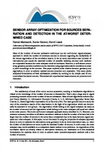
need to generalize the measure defined by (7) for a transformation of arbitrary dimensionality that may be carried out by a chemical sensor array. [Place Figure 2 near here] To do this we need to consider an example transformation for which the sensitivity matrix is not square, as shown in Figure 2. This visualization shows how the cube of unit side within odor space is mapped onto the plane in sensor space. Clearly, in this example the area defining Vs cannot be found by a single determinant. If we consider the three 2 × 2 minors (of order 2) of A then each of these represents how a single face of the cube is transformed into the range. That is, each face of the cube is transformed into a region in sensor space defined by its corresponding minor of A. So, for example, the face of unit area {(0, 0, 0), (0, 0, 1), (0, 1, 1), (0, 1, 0)} in the domain has a transformed area equal ¡ to ¢ the absolute value of the determinant of the 2nd-order minor, abs[ det .52 22 ] = 3, in the range. Furthermore, it is evident from Figure 2 that the total region Vs comprises of the three transformed perpendicular faces of the cube, suggesting the general result Vs =
m m X X p=1 q6=p,q=1
...
m X
c0p c0q . . . c0r abs(|Mpq...r |)
for m > n
(8)
r6=p,r6=q,r=1
where Mpq...r is a minor of order n that is obtained by taking the columns (p, q, . . . , r) of A. Again the absolute value is taken since the areas defined by the minors must be additive. This result can be shown to apply generally (m > n) to any linear transformation between m-dimensional odor space and n-dimensional sensor space and so may be used to calculate the allowable space that may be accessed by a given array for a stimulus volume.[6] For an array of linear chemosensors (8) completely specifies the role of the array tuning in terms of defining the total volume of accessible sensor space, which may be considered as the range of the system as a whole. For instance, applying (8) to the example shown in Figure 2 gives a value for Vs = 8.5 which can be easily verified using elementary geometry.
4. Noise Considerations While the performance of an perfectly specific chemical sensor array (such as one where the off diagonal terms of A are zero) is simple to characterize – by simply measuring the detection limit of the sensors individually – the case for cross-sensitive sensors is less straightforward. In the latter case the overall sensitivity of the array to an individual compound arises from the combined sensitivity of a number of devices. Consequently, it is necessary to understand how these individual sensitivities contribute to the array performance. So far we have considered the transformation carried out by a sensor array to be noiseless, that is, there is a perfect correspondence between points within odor space and points within sensor space. In the noiseless case, the magnitude 8
of Vs is unimportant since it is always possible to perfectly resolve neighboring points in odor space, no matter how close in proximity. In practice, of course, all measurements are limited by noise and so chemical sensors generate a non-reproducible response to the same stimulus. Instead of there being perfect correspondence between odor and sensor space, we must now view the noise process as mapping single points in the stimulus space onto a region (usually small) in sensor space where the likelihood of obtaining a particular measurement is determined by some probability density function. When the noise process is introduced into the transformation, the magnitude of Vs becomes of great importance, since it restricts the total number of discriminable features for a given significance level. [Place Figure 3 near here] In the simplest case, where the noise in each sensor is considered to be independent of both the stimulus and the response magnitude, we may define a confidence interval in sensor space as an m-dimensional hyperellipsoid, where the cross-section along the principal axes is given by, δxi = ±σxi , the standard deviation of the noise (or random error) for sensor i. A representation of the noise process combined with the sensor array transformation is shown in Figure 3 for the 2-sensor case where the region Vs is packed by the error ellipses. After Gardner and Bartlett each ellipse corresponds to a single stimulus point in the domain, the number of ellipses that may be packed into the region Vs gives the Number of Discriminable Odor Features, Nn , a bound for which was given in (3). By also taking into account the accessibility of the sensor space for a defined region of the sensor space, as discussed, we can estimate the number of features which can be discriminated by the array on the average Nn ≈
Vs Vn
(9)
Most importantly (9) provides an estimate of the number of discriminable features that can be coded by a chemosensor array, taking into account both noise and array tuning. The value of Vs limits the access to the sensor space depending upon the dynamic range of the stimulus and the array tuning, through (8). By using the formulæ given for Vs in the linear case, (8), and non-linear case, (23), (as will be discussed in Section 5) it is possible to produce an estimate for Nn for any chemical sensor array. [Place table 1 near here] Of particular interest is how the noise generated in sensor space determines the measurement accuracy of the array to individual components of the odor stimulus. This may be achieved by considering the inverse mapping of noise in sensor space onto odor space. We first define a noise matrix, ηx , which comprises each of the sensor errors as a diagonal matrix of the form σx1 0 ... 0 .. 0 σx2 . ,. ηx = . (10) . . . . . 0 0 . . . 0 σxn 9
We can now quantify the inverse transformation of the noise matrix, ηx , via A−1 so as to generate the noise components in terms of the odor space, to give a corresponding detection limit for each individual odor component, ∆c. This corresponds to solving the system of equations ηx = A∆c for ∆c. Depending upon the form of A there are three possible cases to consider, as shown in Table 1. The most straightforward case is where there are the same number of odor components as there are sensors, which produces a square matrix A, and is of full rank (all sensors are linearly independent but not necessarily orthogonal , if this is not the case then we consider the system to be underdetermined). The overdetermined case occurs when there are more independent sensors than individual chemical compounds. Due to the typically high dimensionality of the stimulus in the case of olfaction, the overdetermined case would not be usual. However it is of direct interest to researchers who use arrays of broadly tuned chemical sensor arrays for single gas analysis or sensing mixtures of gases using such systems. This case is dealt with in Appendix A. More usual in electronic nose systems is the underdetermined case where there are more odor compounds than independent sensors within the array. This case is studied in Appendix B assuming that the distribution of the stimuli is Gaussian. In the case of n = m and A is of full rank there is no loss of dimensionality during the forward transformation – i.e. Vs > 0. A unique two-sided inverse exists, A−1 , and each point within the domain has a 1-to-1 mapping with points in the range (subject to noise constraints) –. Now ∆c = A−1 ηx
(11)
and so the detection limit for the array is simply the noise matrix scaled by the elements of the two-sided inverse of the sensitivity matrix and so is simple to calculate. The solution is then of the form δc11 δc12 . . . δc1n δc21 δc22 . . . δc2n ∆c = (12) .. .. .. ... . . . δcm1
δcm2
. . . δcmn
where each column (δc1i , δc2i , . . . , δcmi )T gives the noise vector for sensor i projected onto odor space and each row (δcj1 , δcj2 , . . . , δcjn ) gives the noise components for each sensor projected onto the odor component j. These noise components may act in the same or opposite directions and so the total squared error for the array is ²2 =
m X n X
δc2ij
(13)
i=1 j=1
whereas the overall contribution of sensor i to error in odor space is ²2xi =
m X j=1
10
δc2ji
(14)
and finally the total error produced by all the sensors for odor component j is ²2cj =
n X
δc2ji
(15)
i=1
The latter expression is particularly important since it provides a measure of the detection limit of the noisy chemosensor array to each compound j in view of the array tuning and noise properties. Finally it is also useful to define a signal-to-noise ratio for neighboring points in odor space. This tells us how easy it will be to discriminate between these points given the array tuning and noise performance. For two given stimuli separated by ∆c0 we see that this corresponds to a sensor response of magnitude ∆x0 = A∆c0
(16)
which leads to the local signal-to-noise ratio for stimulus difference ∆c0 SNR∆c0 =
||∆x0 ||2 tr(ηx ηxT )
(17)
where || • || is the Euclidean vector norm and tr(•) is the matrix trace operation. This measure is extremely useful since it allows us to predict the likelihood of discrimination between two points in odor space using a particular chemosensor array. To apply this theory the experimentalist or practitioner needs to be able to provide suitable values for the parameters within (11) and (17). In particular, measuring values for A and ηx is the key requirement. The sensitivity matrix, A, can be measured directly by varying individual stimulus components and calculating the regression parameters of a linear fit between concentration and sensor response (least squares). Since at this point the model assumes a linear behavior, it is straightforward (although time consuming) to estimate all of the values for A, since the sensitivity of each sensor to a particular compound can be measured independently and then assumed to sum linearly in our model. Therefore, over some linear operating region (often assumed to be for low concentrations), regression parameters for the concentration dependence of each sensor to each compound can be estimated directly from the sensor response data. Of course, the number of individual compounds may be too high to be able to realistically estimate an individual sensitivity between each sensor and each compound. However, note that many compounds may be grouped together to act as a single component (dimension in our model) as long as the sensor responds linearly to the mixture over the operating region. Estimating values for ηx provides more of a challenge since it requires estimation of noise properties in each of the sensors. The model assumes the noise for each sensor is constant over the stimulus range and is independent of noise sources in other sensors (later we will show that we can also deal with stimulus dependent noise properties). This assumption makes estimation of the standard deviation of the noise straightforward. There may be two forms of noise that 11
the practitioner might wish to take account of when using the model. Firstly, intermediate to high frequency noise in the sensor response (arising from instantaneous noise sources in the sensor or interface electronics) which may be quantified from the fluctuations in the time series of data to no stimulus or constant stimulus. Secondly, the reproducibility of response of the sensor to repeated stimulus. This would require repeating identical stimuli many times and quantifying the dispersion of responses in each of the sensors. Since the noise is assumed here to be independent, then the noise can be characterized independently in each sensor. If the noise varies over the stimulus range then some mean value can be assumed for the purposes of the linear model. If any of these restrictions do not seem reasonable given the data available for the sensors being optimized, then a more complex, non-linear model such as those discussed below, will need to be considered.
4.1. 2-sensor 2-odor example Some of the concepts become clearer through a trivialized example of a 2 linear sensor array responding to 2 odor compounds. To simplify the calculations we assume that both sensors have the same noise σ and this is independent of the stimulus or sensor response. The sensitivity matrix is then simply µ ¶ a11 a21 (18) a12 a22 and ηx is
µ
σ 0
0 σ
¶ (19)
and so applying (11) we obtain the solution ∆c =
σ a11 a22 − a12 a21
µ
a11 a12
a21 a22
¶ (20)
giving the formula for the total squared error for the array as ²2 = σ 2
a211 + a212 + a221 + a222 (a11 a22 − a12 a21 )2
(21)
[Place Figure 4 near here] As an example of performance optimization we might wish to choose a11 , a12 , a21 , and a22 in order to minimize this error. Clearly a unique solution is not possible, but by choosing the sensitivities of one of the sensors, say a1j , to both stimuli, we can visualize the effect on the error as we vary the tunings for the other sensor, say a2j (Figure 4). The results are intuitive by considering the situation when one sensor possesses sensitivity terms which are multiples of the other (i.e. the sensors are identical after normalization). In this case, the array is unable to distinguish between the individual stimuli so the reconstruction error tends asymptotically towards infinity, reflecting the impossibility of 12
discrimination betweem the separate stimuli in this case. This is represented by the ridge along the center of Figure 4, (left), where the ratio between the sensitivity terms a21 : a22 is 2 : 1. If we constrain each of the sensitivity terms to the range [0, 1] (i.e. sensor can only increase in value and its sensitivity is constrained) then the best performance is obtained when a21 = 0 and a11 = 1, that is, when the second sensor is as different as possible from from the first sensor within the specified constraints.
5. Non-linear Transformations Since only a subset of chemical sensors is considered to behave linearly up to some operating limit, it is necessary to extend the methods developed in Sections 3 & 4 so that they may be applied more generally. [Place Table 2 near here] The concentration dependence of the most popular chemical sensor types to be used within electronic nose systems are shown in Table 2. Of these, metal oxide semiconductor sensors are arguably the most widely used in existing systems. These have been modeled by a Power Law, where ri typically lies between 0.6 and 0.8 but may also depend upon the stimulus. Conducting polymer devices are also very popular for use within chemical sensor arrays and these have been described as behaving according to a Langmuir Isotherm model. For these and other non-linear sensors, a sensitivity matrix may be formed in the non-linear case from the Jacobian matrix, A ∂x1 ∂x1 ∂x1 ¯ ¯ . . . ∂c ∂c1 ∂c2 m ¯ ∂x2 ∂x2 . . . ∂x2 ¯ ∂cm ¯ ∂c1 ∂c2 A= . (22) ¯ .. .. .. .. . . . ¯¯ ∂xn ∂xn . . . ∂xn ¯ ∂c1
∂c2
∂cm
c1 ,c2 ,...,cm
for some operating point (c1 , c2 , . . . , cm ) in odor space. This linearized sensitivity matrix may then be used in place of A, as defined by (6) so that the analysis developed in Sections 3 & 4 may then be applied in the general nonlinear case. The determinant of the Jacobian, J = |A|, may then be used to approximate the localized hypervolume for the transformation for a particular operating point. Furthermore, the Jacobian may also be applied to calculate the hypervolume of accessible sensor space in the non-linear case, since Z Vs = 0
c0m
Z ... 0
c02Z c01
J dc1 dc2 . . . dcm .
(23)
0
[Place Figure 5 near here] [Place Figure 6 near here] The fitting of experimental data for the practitioner using these non-linear models is straightforward. Rather than finding the regression parameters that 13
fit the concentration dependence of sensor reponse in the linear case we should now estimate the regression parameters of the model in the general non-linear case. Such non-linear regression can be achieved by most statistical software packages. Because of the nature of the models described in Table 2, the action of each of the compounds still sums linearly (even though their dependence on individual compounds may be non-linear) and so the sensor response to each compound may be analyzed independently. More complex models of analyte competition for sites in each sensor could be developed and may still be applied using the preceding equations, (23) and (22). As with the linear models the noise is considered to be independent of the stimulus. The Fisher information approach, to be described below, should be used in the case of stimulus-dependent noise. Examples of calculations for the noiseless non-linear case are shown for metal oxide semiconductor sensors in Figure 5 and for conducting polymer sensors in Figure 6, using the sensor models summarized in Table 2. For both examples the non-linear mapping of 2-odour space is shown, showing how the non-linearity in each sensor contributes to the transformation as a whole. The nature of the models implies that the metal oxide semiconductor devices are far more linear in their behaviors which is verified by contrast the mappings onto sensor space for both sensor varieties. In particular, the localized volume of the transformation in the conducting polymer case is shown to tend towards zero with increasing stimulus concentration. This is also shown by Figure 6 which shows the linearized Jacobian at different points in the stimulus space. As c1 , c2 → 1, J → 0, verifying the observation. In contrast the determinant of the Jacobian for the metal oxide array never reaches zero, since the behavior of these sensors is more linear. Note that the same analysis on an array of linear sensors would produce a perfectly flat feature localized volume. Hence the localized feature volume map provides an intuitive visualization of the performance of the sensor array in detecting the stimulus.
6. Array Performance as a Statistical Estimation Problem We can also consider the definition of chemosensor array performance in a different context, one which we will show provides certain advantages in the calculation of the array error. Here we consider the data produced by a chemosensor array as being part of a statistical estimation problem as outlined in Figure 7. Each sensor within the array produces a response dependent on its tuning to the stimulus plus some noise. A hypothetical statistical estimator (one produced using for instance maximum likelihood or Bayesian estimation methods) uses the noisy response from the array in order to attempt to reconstruct the stimulus. Due to this noise, if we present several times the same stimulus c to the system, the estimator response ˆ c will not be the same on each occasion but
14
will fluctuate around a certain mean value. An unbiased estimator should be right on the average, that is, if we present many times the same stimulus c, the mean of the different estimations ˆ c should be equal to c. Moreover, the variance of the response of the estimator when the stimulus is fixed should be as small as possible. If the estimator is unbiased, its squared error in the estimation coincides with its variance. [Place Figure 7 near here] Depending upon the tuning parameters of the individual sensor elements and their noise properties, the accuracy of the overall sensor system in estimating the stimulus varies in addition to the range of stimuli that may be appreciated. A typical goal in choosing which sensors to incorporate into an artificial olfactory system is to maximize the accuracy with which the sensory system can estimate/predict the stimulus or optimally discriminate between neighboring stimuli. By considering a hypothetical unbiased statistical estimator that uses the sensor array response in order to estimate the individual stimuli within a complex odor mixture, we can define and test how different tuning parameters of the sensor array effect the accuracy of stimulus reconstruction. This arrangement is shown in Figure 7 where each sensor, i, generates a response xi to the multicomponent stimulus c. Conveniently, our problem when placed in this context is well known to the field of statistical estimation, and classical results exist that we can call upon here. For example, the variance (directly related to the error) of any unbiased estimator that might be constructed for this purpose has a well defined limit through the “Cram´er-Rao bound” which we will make use of.[3] Furthermore a direct relationship between the Cram´er-Rao bound and Fisher information exists that allows us to calculate this bound and therefore quantify the performance of the array in reconstructing the stimulus.
7. Fisher Information Matrix and the Best Unbiased Estimator When a multicomponent odor stimulus c is exposed to the sensor array, the array of sensors gives a response x which component i denotes the response of sensor i. Due to the noise, the array response is not deterministic so it follows some probability density function p(xi |c) conditioned on the stimulus. The elements of the Fisher information matrix (FIM), Jjj 0 (c), are defined as [3] ¶µ ¶ µ Z ∂ ∂ ln p(x|c) ln p(x|c) Jjj 0 (c) = d x p(x|c) (24) ∂cj ∂cj 0 where j and j 0 are both individual stimulus components. Some understanding of what is being measured by the Fisher information can be gained by considering the simplified case of a single sensor responding to a single odor component. For ease of the analysis let us assume that the sensor responds to stimulus concentration with a Gaussian tuning curve (note this is not physically reasonable 15
for a chemosensor but is for illustrative purposes only). In this case we have the situation shown in Figure 8(a). Now (24) reduces to µ ¶2 1 df (c) J(c) = 2 (25) σ dc where f (c) is the mean sensor output to the stimulus c, hx|ci, in this example following the Gaussian curve (see Figure 8a) and σ is the standard deviation of the noise shown as error bars in the same figure. From this simplified example we see that the Fisher information scales inversely with the noise variance but is linearly dependent upon the square of the slope of the tuning curve (here concentration dependence). We see that the slope of the tuning curve is greatest at the inflexion points of the Gaussian, which from (25) is also where the Fisher information is maximum, Figure 8(b). At the peak of the Gaussian where the slope is zero, the Fisher information is also zero, Figure 8(c). This result is intuitive since if we wish to measure a small change in the stimulus it is far better to be operating on the slopes of the tuning curve, where we obtain a relatively large change in sensor output for a given stimulus change, compared to at the peak, where the change in sensor response will be close to zero. So we see that the Fisher information concisely describes the combined role of sensor tuning and noise in defining estimation performance. [Place Figure 8 near here] Although (24) may not be straightforward to interpret directly, we can relate it to the reconstruction error of the stimulus through the “Cram´er-Rao bound”. This states that for every unbiased estimator that uses the data x for estimating ˆ, the squared error for stimulus component j satisfies the stimulus c, as c D E var(cˆj |c) ≥ (J−1 (c))jj ≡ ²2cj (26) opt
where “var” means variance, h•i is the expected value or mean, and cˆj is the estimation of the component j of c, j = 1, . . . m.[3] And so this also provides a valuable link to the geometric theory of array error given by (15). This result allows us to directly calculate the minimum expected reconstruction error for a given stimulus component j from the jth diagonal element of the inverse of the Fisher information matrix. Furthermore, the total expected squared reconstruction error across the entire array is equal to the summation of the errors in each of the components. That is, var(ˆ c|c) =
m X
var(cˆj |c) ≥
j=1
m X
® (J−1 (c))jj = ²2 opt
(27)
j=1
and so the overall performance of the array in detecting all of the stimuli is defined by the elements of the Fisher information matrix, Jjj 0 . In Appendix C we show that the Fisher information and geometric approaches to sensor array optimization are equivalent when the noise in the sensors is independent from the stimulus. In the case of stimulus-dependent noise, the Fisher information approach should be used. 16
There is another notion related to Fisher information called “discriminability”. This measures the ability of the system to distinguish between two similar stimuli c1 and c2. If we call ∆c = c2 − c1, the ability of the system to discriminate between these is given by d 0 ≡ ∆cT F∆c
(28)
The maximization of this quantity can be shown to be equivalent to the maximization of the local signal-to-noise ratio defined in equation 17. We now need to be able to calculate the FIM for different sensor array configurations in order to proceed.
8. Fisher Information Matrix Calculations for Chemosensors Firstly, the FIM for an individual sensor i is given by the elements of the matrix µ ¶µ ¶ Z ∂ ∂ i Jjj 0 (c) = dxi p(xi |c) (29) ln p(xi |c) ln p(xi |c) ∂cj ∂cj 0 It can easily be shown that when the array of sensors has uncorrelated noise, the FIM of the entire array, J, is equal P toithe summation of the individual FIM matrices for each sensor i, that is i J . This is valid in a general sense – in other words the noise and concentration dependence of the sensors can be different across the array and can comprise different sensor technologies, noise properties and tunings. We now calculate the FIM elements for two example cases of chemical sensor by substituting the appropriate probability density function into (29) and rearranging. Case 1: Analog chemical sensor with Gaussian noise: i Jjj 0 (c) =
1 σx2i (c)
∂fxi (c) ∂fxi (c) 1 ∂σxi (c) ∂σxi (c) +2 2 ∂cj ∂cj 0 σxi (c) ∂cj ∂cj 0
(30)
where fxi is the mean response for sensor xi , i.e. fxi (c) = hxi |ci which would be expected to follow some model of concentration dependence, e.g. a simple linear model such as given by Eq. (1) However, the sensor model for the concentration dependence can be a far more complex, non-linear one. Note also that, in principle, the noise dispersion can depend on the stimulus. The Gaussian noise case is most appropriate for describing metal-oxide semiconductor and conducting polymer chemosensors used within electronic nose systems, where the partial derivatives can be calculated for the sensor models given in Table 2. Case 2: Analog chemical sensor with Laplacian noise: i Jjj 0 (c) =
1 αx2 i (c)
∂fxi (c) ∂fxi (c) 1 ∂αxi (c) ∂αxi (c) + 2 ∂cj ∂cj 0 αxi (c) ∂cj ∂cj 0 17
(31)
where αxi (c) is the dispersion parameter of the Laplacian noise for that sensor. The Laplacian case is most appropriate for describing fluorescence-based optical chemosensors used within artificial olfactory systems, where the concentration dependence is approximately linear up to saturated vapor pressures of analyte.[4]
8.1. 2-sensor 2-odor example To illustrate these concepts we again consider two linear sensors to generate an analog response that is corrupted by Gaussian noise, identical to the example given in section 4.1. This is a linear model and so the sensitivity of sensor i to ∂fxi (c) stimulus component j is a constant aij ≡ ∂c . Using (30) we can calculate j the FIMs for each sensor µ ¶ µ ¶ 1 1 a211 a11 a12 a221 a21 a22 1 2 J = 2 J = 2 a11 a12 a212 a21 a22 a222 σ σ Adding these to form the FIM of the array, then substituting into (27) and rearranging we obtain exactly the same form as (21), demonstrating equivalence between the geometric and information theoretic approaches in this case. In Appendix C we show that this equivalence holds for any input dimension.
9. Performance Optimization [place Fig. 9 near here] An outline of the optimization problem we will consider is shown in Figure 9. A pool of k different sensor types is available, each with a unique profile of response to the m distinct molecular species relevant to the problem. Our instrument provides n channels, each of which we can assume may house any of the available sensors. Furthermore, we will not consider duplication of sensor types amongst the array since this yields no additional information about the stimulus, but acts to reduce the noise in the system if averaging is employed (this case can be dealt with for independent noise by replacing the l identical sensors in the calculations with a single sensor of the same type but with noise σ2
variance, σx02i = xl i ). The optimization problem is then to select the single configuration¡ that ¢ provides the best sensing performance to the compounds of interest out of nk = k! n!(k−n)! possible configurations. Best here depends upon the detection task to be solved. We envisage three possible criteria to be optimized in a practical system 1. Maximize the total number of Nn separate features that can be detected by an array. This is optimizing the range of the system and can be directly quantified from the geometric approach (eq. 9). Shannon information theoretic approaches are more suited to calculating this value than the Fisher information. 18
2. Maximize the SNR obtained from the array for some vector or set of vectors in stimulus space. This is optimizing the resolving power or discrimination ability of the array and may be quantified using either the geometric (eq. 17) or Fisher information (eq. 28) approaches. 3. Estimate the concentrations of some of the compounds or some function of these, e.g. interfering compounds (distractors) could be present. This is optimizing the detection threshold of sensitivity for the system to specific components, which can be quantified using either the geometric or Fisher information approaches. The case where we are interested in reconstructing the concentration of all the stimulus compounds has been extendedly described in this chapter.
9.1. Optimization Example We will illustrate the Fisher information maximization principle with a simple example. Consider a set of linear chemosensors each responding to combinations of 3 single odour components (m = 3). The noise in all the sensors available to us is assumed to be Gaussian, independent of each other and the stimulus, and with equal variance. For this example we assume each sensor is available with 5 graded levels of sensitivity to each of the 3 components, that is, 0, 0.25, 0.50, 0.75 or 1.0. Therefore, there are k = 53 = 125 possible sensor types. We would like to select a sensor array consisting of any 3 of these available sensors (that is, n=3). Therefore, we should select those 3 sensors from the 125 available that optimize the performance of the system in terms of the overall reconstruction 125! error (criteria 3 above). For each of the (125−3)! 3! = 317, 750 possible array configurations we calculate the system Fisher information as previously described, in order to evaluate their performances. [Place Table 3 near here] [Place Figure 10 near here] In Table 3 we show the three best groups of solutions. Note that the optimal configuration is formed by sensors with non-zero sensitivities as well as zero sensitivities – they are mixed. The non-zero sensitivities are maximum in each case, showing that intermediate sensitivities are disregarded. This is intuitive, since providing as much gain as possible to each of the analytes will maximize the performance under all three optimization criteria discussed above – increased gain is always advantageous as long as it is not commensurate with equal amounts of noise. Importantly the specific case (in which each sensor responds to a different component with maximum gain while its sensitivity to the others is zero) is not the best in our example (the expected squared error of this configuration is exactly 3σ). This demonstrates that even if it were possible to develop perfectly specific sensors for given compounds, this would not yield the best possible performance for electronic nose systems, since some amount of overlap in sensor response is shown to be advantageous. Interestingly, the sensors forming the optimal configuration tend to have the same number of zero and non-zero sensitivities as the input dimension increases (data not shown). 19
Arrays formed by non-independent sensors (some linear relationship between the sensitivities exists within the array) have infinite expected error since they are not able to between discriminate 3-dimensional stimuli. For example, the singular configuration shown in table ?? has only 2 independent sensors. Therefore, it can only discriminate between 2-dimensional stimuli. The errors of all the 317, 750 possible arrays are sorted and shown in Figure 10. Critically, the error of any given configuration can be orders of magnitude greater than the error of the optimal configuration. Therefore, if the sensory array is designed randomly choosing 3 of the awailable sensors, we are likely select a far-from-optimal configuration. We stress this point to indicate the importance of optimization in chemical sensor array design. For example, the probability of having an expected squared error more than 100 times the optimal one is 22.46% (see Figure 10). The technique illustrated in this example can be analogously used in general conditions: non-linear sensors noise that depends on the stimulus, other types of noise (non-Gaussian), bipolar sensor sensitivities, and arrays of sensors with different kinds of responses and noises [8]. Many more complex examples can be easily constructed.
10. Conclusions In this chapter we have described two unified theories of chemical sensor array performance – using both geometric-based linear algebra and Fisher information approaches. The theories may be applied in a variety of conditions – for different sensor noise properties and different concentration dependence models. More generally, any variety of different sensor types may be optimized within the same array. The geometric theory is particularly suited to visualization of the sensor array performance whilst the Fisher information copes with more complex scenarios, where, for example the sensor noise is dependent on the stimulus. The utility of the approaches for array optimization is demonstrated using a number of simple examples that serve as the basis for more realistic applications of the theory. Manufacturers of electronic nose instruments may easily apply this theory in order to optimize the sensing performance of the systems they sell. Furthermore, we can envisage a catalog of parameters for each sensor used within practical systems today which would make the optimization of sensor arrays to particular detection tasks a simple and routine operation.
11. Acknowledgments T.C.P. was supported by grant IST-2001-33066 from the European Commission and GR/R37968/01 from the United Kingdom Engineering and Physical Sciences Research Council. M.A.S.-M. was supported by grant BFI2000-0157 from MCyT.
20
References [1] Zaromb S. & Stetter J.R., Theoretical basis for identification and measurement of air contaminants using an array of sensors having partly overlapping selectivities. Sensors & Actuators, 6 (1984), 225-243. [2] Gardner J.W. & Bartlett P.N., Performance definition and standardization of electronic noses. Sensors & Actuators B, 33 (1996), 60-67. [3] Cover T.M. & Thomas J.A., Elements of Information Theory, John Wiley, 1991. [4] Pearce T.C., Verschure P.F.M.J, White J., Kauer J.S., Robust Stimulus Encoding in Olfactory Processing: Hyperacuity and Efficient Signal Transmission, in Neural Computation Architectures Based on Neuroscience, eds. Wermter S., Austin J., and Willshaw D., Springer-Verlag, 2001. [5] Wicks J.R., Linear algebra an Interactive Approach with Mathematica., Addison-Wesley, 1996. [6] Wicks J.R., personal communication. [7] Pearce T.C., Odor to sensor space transformations in biological and artificial noses, Neurocomputing, 32-33 (2000), 941-952. [8] S´anchez-Monta˜ n´es M.A., Pearce T.C., Fisher Information and Optimal Odor Sensors, Neurocomputing, 38-40 (2001), 335-341.
A. Overdetermined Case The Fisher information approach described in the main text operates correctly in the overdetermined case. However, for the geometric approach described in the main text, we must find the least squares solution which leads to ∆c = (AT ηx−2 A)−1 AT ηx
(32)
and ²2 =
n X m X
∆c2ij
(33)
i=1 j=1
It can be easily verified that when A is square these equations are the same as (11) and (13) respectively.
21
B. General Case with Gaussian Input Statistics The global optimal estimator is that which minimizes the global expected error. When the sensors are linear and the noise is Gaussian this minimum error can be shown to be tr((AT ηx −2 A + V−1 )−1 ), where V is the covariance matrix of the input stimuli, which are assumed to be Gaussian distributed. This equation is valid for all the cases (square A, undetermined and overdetermined cases) as well as when the input statistics are not homogeneous and so is the most general result.
C. Equivalence Between the Geometric Approach and the Fisher Information Maximization Since
P i,j
x2ij = tr(xxT ), and using (32) and (33) can be rewritten as
²2 = tr((AT ηx −2 A)−1 AT ηx ηx T A((AT ηx −2 A)−1 )T ) = tr((AT ηx −2 A)−1 ) (34) On the other hand, if the sensors are linear and their noise does not depend on the stimulus, the equations 30 and 31 can both be expressed as −2 i Jjj 0 (c) = (ηx )ii aij aij 0
(35)
Then the total Fisher information matrix is J = AT ηx −2 A so by equation (27) the optimal error is simply tr((AT ηx −2 A)−1 ), which coincides with that derived for the geometrical approach. A similar proof can be shown for when the sensors are non-linear.
22
Odor Space
Sensor Space
c2
x2
1 0 A= =I 0 1 c1
Vo=1
(a) c2
.75 .25 A= .25 .75
c1
c2
.75 .55 A= .55 .75 (c)
(d)
Vs= 0.5
x1
x2
c1
Vo=1 c2
.75 .75 A= .75 .75
x1
x2
Vo=1
(b)
Vs=1
Vs= 0.26
x1
x2
c1
Vo=1
Vs= 0
x1
Figure 1: Visualization of a 2-odour to 2-sensor transformation for different examples of linear sensitivity matrices, A, a) orthogonal sensors through to, d) identical sensors. Vo : Hypervolume of accessible odor space, Vs : Hypervolume of accessible sensor space. (Reprinted with permission from Pearce 2000,[7])
23
�������� �� �� c
����� ������� �� �� x2
Vo= 1
2
1 (0,1,0)
Vs= 8.5
5
(1,1,0)
(1,1,1) (0,1,1)
4 (0,1,1)
3
(1,1,1)
2
1 (0,0,0)
(1,1,0)
(1,0,1)
(0,1,0)
(1,0,0)
c1
(0,0,1)
1
(1,0,0)
1 c3
(0,0,1)
(1,0,1)
(0,0,0)
1
2
3
4
5
Figure 2: Visualization of a 3-odour to 2-sensor transformation �
x2= 2
x
�
x1= 1
x2
�
x1
Figure 3: Sensor space representation where sensor noise has been represented as ellipses superimposed on the region Vs . The addition of the noise components for each sensor δxi = σxi . For illustration purposes we assume here that the noise is independent of the stimulus or sensor response. (Reprinted with permission from Pearce 2000 [7]). 24
x1
Table 1: Models of concentration dependence for a variety of chemical sensors and their behaviors. All models assume that no competition for sites within sensor takes place, and that chemicals act independently on the sensor. (Reprinted with permission from Pearce 2000 [7]). Model PLinear m x = j=1 aj cj + a0
Behaviour
Sensor Response, x
Device Electrochemical Fuel Cell, Fluorescent Indicators
20 15
10 5
0 0
2
4
6
8
10
8
10
Concentration, c j
x=
Power Pm r j=1 aj cj + a0 Sensor Response, x
Metal Oxide Semiconductor
10
8
6
4 0
2
4
6
Concentration, c j
x=
Langmuir Pm bj aj cj j=1 1+aj cj
+ a0 Sensor Response,x
Conducting Polymer
3.8 3.6 3.4 3.2 3 0
2
4
6
8
Concentration, c j
25
10
Table 2: Possible cases of transformations between odor and sensor space, showing examples for each case. Odor space
Sensor Space
n=2
m=2 c2
x2
x2
c2 x1
x2 c1 c1
Uniquely Determined (n = m) ∪ (Vs > 0)
x1
x1
n=2 x2
m=1 x2 x1
Overdetermined (n > m)
x2
c1
x1
m=3
n=2
c2 x2
x2
x1
Kernel
c1 26 Underdetermined (m > n) ∪ (n = m ∩ Vs = 0)
c3
x1
x2 x1
x1
0
a21
0.2 0.4
0.6 0.8 4
1
3 2 Log e �
2 1 0
0 0.2 0.4 0.6
a 22
0.8 1
Figure 4: The effect on the optimal squared by estimation error, ²2 , to variations in the tuning of one sensor within an odor sensing array of two sensors after fixing the sensitivities for the other sensor. The array is composed by 2-linear sensors with Gaussian noise, where the tunings of one of the sensors is fixed, a11 = 1, a12 = 0.5. (Reproduced with permission from S´anchez-Monta˜ n´es & Pearce, 2001 [8])
Sensitivities Sensor 1 Sensor 2 Sensor 3 2® ²
a1 0 1 1
Best a2 1 0 1 2.25
a3 1 1 0
a1 0 1 1
2nd Best a2 a3 0.75 1 0 1 1 0 2.51
a1 0 1 1
3rd Best a2 a3 1 1 0.25 1 1 0 2.65
a1 0.5 0.25 0.25
Singular a2 a3 0.25 1 0 0.25 0.25 0.75 inf
Table 3: Best 3 groups of solutions in the optimization example, and one singular solution (dependent sensors). The errors are given in units of the noise variance. The best error is achieved by just one solution (shown in the table), while the 2nd best error and 3th best error are each achieved by 6 solutions (corresponding to replace a 1 sensitivity with 0.75 and 0.25 respectively). The table shows instantiations of these suboptimal solutions.
27
Odor Space yc2 axis
Sensor Space
Domain
x2 axis
1
Range
�
0.7 0.6
0.8
0.5 0.6
0.4 0.3
0.4
0.2 0.1
0.2
x1 axis �
0.2
0.4
0.6
0.8
1
0.2
c1 axis
0.4
0.6
0.8
1
(a)
J, Feature Volume 0.8 0.6 0.4 0
0 0.2
0.2 0.4
0.4 0.6 c2
0.6 0.8
0.8
c1
1
(b) Figure 5: (a) Visualization of 2-odor to 2-sensor transformation using the nonlinear Power Law model for metal oxide semiconductor devices: x1 = a11 cr11 + a12 cr21 , x2 = a21 xr12 + a22 cr22 , where r1 = r2 = 0.8 and a11 = 0.8, a12 = 0.25, a21 = 0.6, and a22 = 0.25 (b) plot of the determinant of the Jacobian for the same 2-sensor metal oxide device array showing how the localized feature volume varies with the stimulus. (Reprinted with permission from Pearce 2000)[7]).
28
Odor Space
Sensor Space x2 axis
x ��� �axis
Domain
Range
0.7
1
0.6 0.8 0.5 0.6
0.4
0.4
0.3 0.2
0.2
0.1 0.2
0.4
0.6
0.8
1
c1 axis 0.1
0.2
0.3
0.4
0.5
x1 � axis
(a)
0.3 J, Feature Volume 0.2 0.1
0
0 0.2
0
0.2 0.4
0.4 0.6 c2
0.6 0.8
0.8
c1
1
(b) array showing how the localized feature volume varies with the stimulus. (Reprinted with permission from Pearce 2000)[7]). Figure 6: (a) Visualization of 2-odour to 2-sensor transformation using the non-linear Langmuir Isotherm model for conducting polymer devices: x1 = a11 c1 a12 c2 a21 c1 a22 c2 1+a11 c1 + 1+a12 c2 , x2 = 1+a21 c1 + 1+a22 c2 , (b) plot of the determinant of the Jacobian for the same 2-sensor conducting polymer device array showing how the localized feature volume varies with the stimulus. (Reprinted with permission from Pearce 2000)[7]).
29
Sensor Parameters
c1 c^2 c^3
Estimator
.....
c1
c3
Sensor
.....
. .. .. .. .
^
x1 x2 x3 x4 x5
Array
cm
c
. . . . .. . .
c^3
1
c
Array Response
Estimated Stimulus
x
Noise
c^
^ m
xn
Stimulus
^
c2
.....
c1 c2 c3
c 2.
Estimator Parameters
c^
Figure 7: A hypothetical statistical estimator takes the response vector, x, from a sensor array and uses this in order to estimate (reconstruct) the stimulus. The tuning parameters for each of the sensors are represented as parameters to the sensor array. (Reproduced with permission from S´anchez-Monta˜ n´es & Pearce, 2001 [8])
1
1
Sensor response
Sensor response
Sensor response
1
0.8
0.8
0.8
0.6
0.6
0.6
0.4
0.4
0.4
0.2
0.2
0.2
0 10
15
20
25
30
35
40
Stimulus
(a)
0 10
15
20
25
Stimulus
(b)
30
35
40
0 10
15
20
25
Stimulus
30
(c)
Figure 8: In this example the sensor is characterized by (a) a bell-shaped tuning curve with overlapping Gaussian noise. The bars show the standard deviation of the noise. (b) The points that maximize Fisher information are those where the slope of the receptive field is higher. (c) Points where the slope is zero make the Fisher information minimum.
30
35
40
� �#�� $� "% $���&�('�� "� �)� * � ����� ���,+-� '��)�
.
����������
/ 0 �������� �� ���������������������� �! "����� ���� �
�
Figure 9: A cartoon of the optimization problem for chemical sensor arrays.
31
Expected Square Error
1000.0
800.0
600.0
400.0
200.0
0.0
0
100000
200000
300000
Rank Configuration Figure 10: Expected squared error for all possible sensor array configurations. The configurations are ranked according to their squared error. The grey zone indicates solutions with infinite error (dependent sensors). The error is normalized by the best expected squared error. Dotted line indicates the configuration in which the squared error starts to be greater than 100. The percentage of configurations whose error is greater than 100 is 22.46%.
32