Computing a High Depth Point in the Plane. Stefan Langerman, William Steiger. Department of Computer Science, Rutgers University. Abstract Given a set S ...
Metrika manuscript No. (will be inserted by the editor)
Computing a High Depth Point in the Plane Stefan Langerman, William Steiger Department of Computer Science, Rutgers University
Abstract
Given a set S = {P1 , . . . , Pn } of n points in Rd , the depth δ(Q)
of a point Q ∈ Rd is the minimum number of points of S that must be in a closed halfspace containing Q. A high depth point is a point whose depth is at least maxi [δ(Pi )]. For dimension d = 2 we give a simple, easily implementable O(n(log n)2 ) deterministic algorithm to compute a high depth point and we give an Ω(n log n) lower bound for this task.
1 Introduction and Summary Given a set S = {P1 , . . . , Pn } of n real numbers, the depth of x ∈ R is defined to be d(x) = min(|{Pi ≤ x}|, |{Pi ≥ x}|),
(1)
and may be thought of as the “size” of the smallest halfspace containing x. A median is a point of maximal depth (d(n + 1)/2e) and may be found in O(n) time.
2
Stefan Langerman, William Steiger
There are many situations where multivariate generalizations of ranks and order statistics are useful, and several suggestions for depth in Rd have been made (Chazelle [2], Gill et. al. [8], Rousseeuw and Hubert [14], Rousseeuw and Hubert [15]). One of the more familiar ones was proposed by John Tukey [17], a natural extension to d > 1 of the notion in (1). Given a set S = {P1 , . . . , Pn } of n points in Rd , the Tukey depth, or simply depth of x ∈ Rd is defined by
δS (x) = min (du (x)) u:kuk=1
(2)
where du (x) is the directional depth of x in direction u and is defined as the depth (as in (1)) of the Pi projected orthogonally onto the line {x + tu, t ∈ R}. Clearly δS (x) measures the smallest number of points of S in any halfspace containing x, and we could take
δS (x) =
min halfspace
|h ∩ S|
(3)
h3x
as the definition of Tukey depth. When the set that defines depth is clear we write δ for δS . A median is a point µ of maximal depth, and we write δ ∗ = δS∗ for the Tukey depth of a median. For integer k > 0 let Ck (S) ⊂ Rd denote the set of points of depth at least k. Then δ ∗ = max (k : Ck (S) 6= φ).
(4)
It follows from (3) that Ck (S) is convex. A well known consequence of Helly’s Theorem (e.g., Edelsbrunner [7]) is that there is a point x ∈ Rd
Computing a High Depth Point in the Plane
3
(not necessarily in S) of depth at least dn/(d + 1)e. Such a point is called a centerpoint. The center is the set of all centerpoints. The question addressed in this paper is related to the computational complexity of selection; that is, finding points of a given depth k, or finding points of maximal depth δ ∗ = δS∗ , along with the value of δ ∗ . Clearly dn/(d + 1)e ≤ δ ∗ ≤ d(n + d)/2e. We use the unit cost RAM model of computation in which every arithmetic operation (+, −, ∗, /) and each binary comparison is assigned a unit cost. A centerpoint in Rd can be found by solving a set of Θ(nd ) linear inequalities, using linear programming (Clarkson et. al. [3]). When d = 2 the situation improves. Cole, Sharir and Yap [6] described an O(n(log n)5 ) algorithm to construct a centerpoint, and subsequent ideas of Cole [4] could be used to lower the complexity to O(n(log n)3 ). Recently, Jadhav and Mukhopadhyay [9] described a linear time algorithm to find a Tukey centerpoint. Matouˇsek [11] attacked the harder problem of computing a Tukey median. Let us first observe that a “brute-force” approach could compute a point of maximum depth in O(n4 ): The N = lines which subdivide the plane into
� N 2
�
n 2
pairs of points define N
convex cells. The points in each
cell have the same Tukey depth and the max can be found in O(n4 ) using Lemma 1 from the next section. Matouˇsek first described an O(n(log n)4 ) algorithm that gives a description of Ck (S), k ≥ dn/3e. Then, using this in a binary search on k ∈ [dn/3e, d(n + 2)/2e], the largest k for which Ck (S) 6= φ is found in O(n(log n)5 ). Langerman and Steiger [10] described an algo-
4
Stefan Langerman, William Steiger
rithm that can compute a median in O(n(log n)4 ), and recently improved it to O(n(log n)3 ). It would not be easy to implement any of these algorithms and all have large constants hidden in the O(). The contribution of the present paper is a simple, easily implemented algorithm to compute a deep point in the plane. We call a point Q “deep” if δ(Q) ≥ δ(Pi ) for all points Pi ∈ S. Note that Q need not be a point in S. Deep points should be useful, in view of the interest in maximal depth points and in the apparent difficulty in obtaining them. Specifically we prove Theorem 1 Given n points in general position in R2 , in time O(n(log n)2 ) a deep point Q can be found along with δ(Q), its depth. There is not much scope for improvement in view of the Ω(n log n) lower bound we establish for finding a deep point and reporting its depth. Theorem 2 An algebraic decision tree to decide whether a deep point has depth ≥ (n + 1)/2 has height Ω(n log n). Theorem 1 is proved via an algorithm having the asserted complexity. It is quite simple and easy to implement, using (i) the O(n) centerpoint algorithm or some randomized variant, (ii) an O(n log n) algorithm to compute the depth of a given point, and a pruning strategy. The lower bound is via a connected components argument. If the points of S are in convex position a deep point Q could have depth δ(Q) = 1, not really deep. It would be easy to modify Theorem 1 to return a deep point of depth at least n/3 by computing in O(n) time a centerpoint
Computing a High Depth Point in the Plane
5
A and then running the algorithm on S ∪ A. Finally, we describe a version of these results for points in Rd , d > 2.
2 Finding a Deep Point in the Plane Given S = {P1 , . . . , Pn }, n points in general position in the plane, the goal is to construct a point whose depth is at least that of any point in S. As is often the case with selection problems, it will be useful to look at the corresponding ranking problem, in this case computing the Tukey depth δ(Q) for some input point Q Here is a natural algorithm, described by Rousseeuw and Ruts [16], but which appeared implicitly in the parametric search in Cole, Sharir, and Yap [6]: 1. Sort the points in S in the order of the slopes of the lines joining them to Q in O(n log n) time. 2. Rotate a line about Q, keeping track of the number of points on each side of the line. Record the minimum number during the rotation, in O(n) time. 3. When the line has returned to its original position, the recorded number is the depth of Q. This algorithm runs in O(n log n) time. Note that if δ(Q) = k, then there must be a closed halfspace through Q containing exactly k points of S. Such a halfspace will be called a witness halfspace for Q. If the Tukey depth of a point is thought of as an indicator of quality for this point as a representative of a set, a well behaved set might be expected
6
Stefan Langerman, William Steiger
to contain a good representative of itself, and thus a point of high Tukey depth. This motivates the notion of a deep point, which we restate here: Definition 1 A point Q ∈ R2 is a deep point for a set S if δ(Q) ≥ δ(P ) for every P ∈ S. A deep point could be found by the brute force algorithm in O(n2 log n) by computing the depth of every point in S. In order to reduce that running time, we use the following: Fact 1 If h is a witness halfspace for the point Q, then for any point P ∈ h, δ(Q) ≥ δ(P ). This follows from equation (3): δ(q) ≤ |h ∩ S| = δ(p). We now describe an algorithm that actually solves a slightly more general problem: given a set S of n points, and a set A∗ of candidate points, the algorithm returns a point Q such that δS (Q) ≥ δS (P ) for every P ∈ A∗ . If A∗ is set to S, the algorithm returns a deep point of S. The algorithm maintains a set A of points “to beat” and works as follows: Algorithm Deep(S,A∗ ) A ← A∗ ; P ∗ ← any point of A∗ . while A 6= φ repeat find a point Q ∈ A such that δA (Q) ≥ c|A| for some constant c, 0 < c ≤ 1/3. (e.g. a centerpoint of A) compute δS (Q). Let h be a witness halfspace for Q in S. if δS (Q) ≥ δS (P ∗ ) then P ∗ ← Q endif.
Computing a High Depth Point in the Plane
7
A ← A − (A ∩ h) endwhile Lemma 1 In time O(|A∗ | + n log n log |A∗ |) the algorithm returns a point Q of depth δ(Q) ≥ δ(P ), all P ∈ A∗ . Proof: The invariant of the algorithm is that δS (P ∗ ) ≥ δS (P ) for all P ∈ A∗ − A. The invariant is true at the beginning since A∗ − A = φ, and the invariant is preserved after each step of the while loop: by Fact 1, δS (P ∗ ) ≥ δS (P ) for all P ∈ (A ∩ h). For the running time of the algorithm, note that |A ∩ h| ≥ c|A| because δA (Q) ≥ c|A|. This means that the size of A reduces by a constant factor at every step of the loop, and so there are at most O(log |A∗ |) loop traversals. Each traversal takes time O(T (A) + n log n); T (A) is the time needed to find a point Q, guaranteed to have depth δA (Q) ≥ c|A|, and O(n log n), the time to compute its exact depth as defined by the points in S. We may take T (A) = O(|A|) using the centerpoint algorithm of Jadhav and Mukhopadhyay and observe that the overall running time is ≤
X
K(ci |A∗ | + n log n),
i
t K > 0 a constant, the sum starting at i = 0 with O(log|A∗ |) terms. u As an example if A∗ = S, then the algorithm will construct a high depth point in O(n(log n)2 ) time, as claimed in Theorem 1. This method can be easily generalized to find high depth points in Rd . Finding a point Q ∈ A such that δA (Q) ≥ c|A| can be done in any fixed
8
Stefan Langerman, William Steiger
dimension in time O(|A|) for some suitably small positive constant c [3]. The next step of the algorithm, finding a witness halfspace, can be done in O(nd−1 + n log n) [1], and all the other steps take O(n) time, so the total running time for finding a high depth point in Rd is O(nd−1 log n + n(log n)2 ). Remark: These algorithms are practical. The O(n) centerpoint algorithm of Jadhav and Mukhopadhyay is easily implemented using the linear-time, separated ham-sandwich cut algorithm of Megiddo [12]. Alternatively, we could compute in constant time, a centerpoint of a random sample of size (say) 100 and this would have depth at least n/4 with high probability. Using this for the pruning in the algorithm for Theorem 1, we will have a simply implemented randomized algorithm which has the asserted running time with high probability.
3 The Lower Bound Given a set S of n points in the plane, let δ ∗ denote the depth of a median. We show that Lemma 2 The height of an algebraic decision tree T that can decide if δ ∗ > n/2 is Ω(n log n). Lemma 2 implies Theorem 2 because if a median were actually a point of S, a deep point would have to have the same depth. Proof: Let C denote the circumference of the unit circle in R2 and let T denote an algebraic decision tree (see e.g., Preparata and Shamos [13]) that
Computing a High Depth Point in the Plane
9
can decide whether δ(S) ≥ d(m + 1)/2e for a set S of m points in R2 . We restrict attention to sets S with P0 = (0, 0) and Pi = (cos zi , sin zi ) ∈ C, i = 1, . . . , 4n + 3, zi ∈ [0, 2π]. These restricted inputs can be encoded by points (z1 , . . . , zm−1 ) ∈ [0, 2π]m−1 . We argue that the subset Y ⊆ [0, 2π]m of restricted inputs where T returns YES has Ω(n!) path connected components.
4j
P0
k
Let
� θi =
i 4n + 3
k+1
� 2π, i = 1, . . . , 4n + 3.
(5)
This encodes a set S with m = 4n + 4 points, 4n + 3 of them equally spaced on C, and no two of them diametric in C. The diameter containing Pi , i > 0, is a halving line and both its closed halfspaces contain 2n + 3 points of S. A diameter containing no Pi , i > 0, is a non-halving diameter and has one closed halfspace with 2n + 2 points and the other with 2n + 3 points, so δ(P0 ) is 2n + 2. This is maximal because for any x 6= P0 the line through x perpendicular to xP0 has a closed halfspace with less than 2n + 2 points of S.
10
Stefan Langerman, William Steiger
For inputs to T , we take P0 and 4n + 3 other points encoded via the set I, where z = (z1 , . . . , zm−1 ) ∈ I if all zi ∈ [0, 2π] and zj = θj , j ≡ 1, 2, 3 mod 4}. Let π and ρ be two different permutations of the integers 4, 8, . . . , 4n, and define inputs zπ ∈ I by (θ1 , θ2 , θ3 , θπ1 , . . . , θ4n−1 , θπn , θ4n+1 , θ4n+2 , θ4n+3 ) and input zρ ∈ I by (θ1 , θ2 , θ3 , θρ1 , . . . , θ4n−1 , θρn , θ4n+1 , θ4n+2 , θ4n+3 ). Both zπ and zρ are in Y ∩ I, as they describe the m points in S, but in different order. They are in different components because on a continuous path from zπ to zρ in I, some z4j must “cross” (i.e., reverse its radial ordering) a neighbor, θ4j−1 or θ4j+1 (see figure). Write k = 4j + 2n + 1 mod (m + 1); θk and θk+1 are the neighbors of the diameter through θ4j . If θ4j crosses a neighbor, it first will cross the diameter through θk or the diameter through θk+1 . After this occurs, that diameter will have closed halfspaces with 2n + 2 points on one side and 2n + 4 on the other, and the depth of P0 described by this input z ∈ I will be δ(S) = 2n + 1, so z 6∈ Y . Therefore Y ∩ I has ≥ n! different components. As m = 4n + 3, the height of T is Ω(m log m). u t
References 1. M.W. Bern and D. Eppstein. Computing the depth of a flat. Proc. 12th Symp. Discrete Algorithms, 700-701, (2001).
Computing a High Depth Point in the Plane
11
2. B. Chazelle. Geometric Order statistics. Proc ACM Geometry, 1988. 3. K. L. Clarkson, D. Eppstein, G. L. Miller, C. Sturtivant, and S.-H. Teng. “Approximating center points with iterative Radon points” Internat. J. Comput. Geom. Appl. 6, 357-377 (1996) 4. R. Cole. Slowing Down Sorting Networks to Obtain Faster Sorting Algorithms. J. ACM 34(1), 200-208, (1987). 5. R. Cole, J. Salowe, W. Steiger, and E. Szemer´edi. An Optimal Time Algorithm for Slope Selection, SIAM J. Comp. 18, 792-810 (1989). 6. R. Cole, M. Sharir, and K. Yap. On k-Hulls and Related Problems. Siam J. Comput. 16(1),61-77, (1987). 7. H. Edelsbrunner. Algorithms in Combinatorial Geometry. Springer-Verlag, Berlin, 1987. 8. J. Gill, W. Steiger, and A. Wigderson. Geometric Medians, Discrete Math. 108, 37-51. (1992), 9. S. Jadhav and A. Mukhopadhyay. Computing a Centerpoint of a Finite Planar Set of Points in Linear Time. Discrete and Comp. Geom. 12, 291-312. (1994). 10. S. Langerman and W. Steiger. Computing a Maximal Depth Point in the Plane. Japan Conference on Discrete and Computational Geometry 2000, p46, (2000). 11. J. Matouˇsek. Computing the Center of a Planar Point Set. Discrete and Computational Geometry: Papers from the DIMACS Special Year Amer. Math. Soc., J.E. Goodman, R. Pollack, W. Steiger, Eds, (1992), 221-230. 12. N. Megiddo. Partitioning with Two Lines in the Plane. J. Algorithms 6, 430–433, 1985. 13. F. Preparata and M. Shamos. Computational Geometry. An Introduction. Springer-Verlag, New York, 1985.
12
Stefan Langerman, William Steiger
14. P. Rousseeuw and M. Hubert. Depth in an Arrangement of Hyperplanes. Discrete and Comp. Geom. 94, 388-402 (1999). 15. P. Rousseeuw and M. Hubert. Regression Depth. J. Amer. Statist. Assoc. 94, 388-402 (1999). 16. P. Rousseeuw and I. Ruts. Algorithm AS 307: Bivariate Location Depth. Applied Statistics (JRSS-C), 45, 516–526 (1996). 17. John Tukey. “Mathematics and the Picturing of Data”. International Conf. of Mathematicians, Vancouver, 1975.