Revised CAD LP-99-080
Former title: Animating and sweeping polyhedra along interpolating screw motions
5/1/00
Computing and visualizing pose-interpolating 3D motions Jarek R. Rossignac GVU Center and College of Computing, Georgia Institute of Technology 801 Atlantic Drive, NW, Room 241,Atlanta, GA 30332-0280 Tel: +1-404-894-0671, Fax: +1-404-894-0673,
[email protected]
Jay J. Kim School of Mechanical Engineering, Hanyang University, Seoul, Korea Tel: +822-2290-0447, Fax: +822-2298-4634,
[email protected]
Abstract CAD and animation systems offer a variety of techniques for designing and animating arbitrary movements of rigid bodies. Such tools are essential for planning, analyzing, and demonstrating assembly and disassembly procedures of manufactured products. In this paper, we advocate the use of screw motions for such applications, because of their simplicity, flexibility, uniqueness, and computational advantages. Two arbitrary control-poses of an object are interpolated by a screw motion, which, in general, is unique and combines a minimum-angle rotation around an axis A with a translation by a vector parallel to A. We explain the advantages of screw motions for the intuitive design and local refinement of complex motions. We present a new, simple and efficient algorithm for computing the parameters of a screw motion that interpolates any two control-poses and explain how to use it to produce animations of the moving objects. Finally, we discuss a new and efficient variant of a known procedure for computing a set of faces which may be used to display the 3D region swept by a polyhedron that moves along a screw motion. Keywords: Animation, Assembly, Screw motion, Minimal rotation, Swept region, Polyhedron
INTRODUCTION CAD systems provide a rich variety of techniques for designing models of surfaces or solids and for combining them into large assemblies for digital mock-up or entertainment applications. Many design activities also involve the design of rigid body motions. In some applications, these motions are tightly constrained by function or aesthetics. For example, manufacturing plans may involve representations of precise cutter trajectories [Blackmore92, Boussac96]. Manufacturing automation modules may carry representation of the hierarchical motions of articulated robots. Artistic applications [Witkin88] may call for physically correct or emotionally charged animations. In such applications, motions are formulated in terms of precise or abstract constraints that make manual editing unnecessary, impractical, or tedious. In this paper, we focus on a different breed of applications, where engineers or animators must quickly design series of loosely constrained motions that interpolate two or more control-poses. Examples include the creation of animations that slowly explode CAD models to reveal their internal structures, that show how parts must be handled and assembled for online maintenance manuals, or that define camera trajectories for design verification using walkthrough of virtual mock-ups. We propose a simple technique for computing such interpolating motions, for animating them, for refining and adjusting them progressively, and for displaying the boundary of the region swept by the moving object.
REQUIREMENTS FOR A MOTION EDITOR In this section, we discuss which features are important in an interactive motion-design system for the applications outlined above. Throughout this paper, we assume that the moving shape is a rigid body called the object. We also assume that it is subject to a continuous movement called the motion. We use the term pose to refer to the position and orientation of the object at any given time during the motion. The terms initial pose and final pose refer respectively to the poses at the beginning and the end of the motion. The terms control-pose refers to any pose specified by the designer that has to be interpolated by the motion. Thus the initial and final poses are key-poses. We will not discuss here the speed at which the animation is to be performed. (Speed control may be achieved in a variety of ways. For example, the designer may attach a time and a time derivative to each control-pose, which usually suffices for synchronizing several motions and for creating dynamic effects of decelerations that delineate consecutive motion components.) We will focus on the geometry of the motion. We also assume that the control-poses are ordered. Key-frame interpolations have been used in animation [Witkin88] and robotics, where motions of objects are specified by their initial and final control-poses, and possibly by an ordered series of intermediate control-poses that should be
LP-99-080
Revised on 5/1/00
J. Rossignac and J. Kim
2
interpolated during the motion. But the motions they define are either dependent on the coordinate system, on the process through which the control-poses were created, or on the structure of a hierarchical description of an assembly or scene. We believe that motion designers should be able to use direct manipulation techniques to specify the starting and ending poses, or even a sequence of control-poses to be interpolated, and should not have to worry about coordinate systems or complex motion sequences and parameters. To be intuitive, the interpolation technique must satisfy several constraints, which are discussed in more detail below: • The motion that interpolates two consecutive control-poses must be intuitive and easily predicted by the designer from the two control-poses, independently of the process through which the control-poses were achieved. • The interpolation should not depend on the choice of a coordinate system. • The motion should not be affected by the decision to interpolate intermediate control-poses that are identical to poses already adopted during the motion. We argue that many motion construction models do not provide such functionality. We also point out a common misunderstanding of the concept of motion smoothness, which cannot guarantee smooth trajectories for all points on a model.
Interpolation should be independent of the design history A rigid body motion is a continuous mapping from the time domain to a set of poses. To relieve the designers from the burden of specifying this mapping in abstract mathematical terms, combinations of simple rigid-body motionprimitives, such as linear translations or rotations around the principal axes, are often used. These simple motions are planar and thus ill-suited, by themselves, for approximating arbitrary motions in 3D-space. Specifying combinations of them that should occur in parallel to produce a 3D motion is difficult and error prone, because each rotation and translation is expressed in a different coordinate system produced by the cumulative effect of the previous motion primitives in the sequence. For example, Figure 1a (left) shows the superposition of several instances of a simple object moving along a natural motion that interpolates the initial to final control-poses. The trajectory of the object is not surprising. The final control-pose may have been specified by the designer interactively by starting with the object in its initial pose and applying a series of rigid body transformations (such as translations and rotations around the three principal axes). For example, the final pose may be the result of a translation by v, followed by a rotation of an angle x around the X-axis, followed by a rotation of an angle y around the Y-axis, followed by a rotation of an angle z around the Z-axis. A continuous motion from the initial to the final pose could be produced by animating each transformation, one after the other. For example, the object would first move along a straight line, then be rotated around the X-axis, and so on. This piecewise-simple motion would be unacceptable in many applications. The popular alternative is to animate all the transformations in the sequence simultaneously, and to combine them for each value of time. A linear interpolation of the parameters of each transformation in this sequence would yield a parameterized transformation, which combines a translation by tv with rotations of angles tx, ty, and tz around the three principal axes. As we vary t between 0 and 1, the combined transformation smoothly moves the object from its initial pose to the final one. Unfortunately, as shown in Figure 1b (right), the resulting trajectory may be rather surprising. The unexpected behavior shown here corresponds to a poor choice of the three angles x, y, and z, which may have resulted from an interactive adjustment of the final pose through trial-and-error. For example, the same final pose may have been obtained by replacing x by π-x and adjusting the other two angles accordingly. We advocate that the natural interpolation of Figure 1a should be computed automatically from the two control-poses.
Figure 1: Screw motion on the left (a) versus linear interpolation of pose parameters right (b)
LP-99-080
Revised on 5/1/00
J. Rossignac and J. Kim
3
Interpolations should not depend on the coordinate system Natural motions, such as the one shown in Figure 1a , are produced by interpolations that involve a minimum angle rotation for which the direction of the axis of rotation is defined (as discussed below). However, there is a choice for selecting the location of the axis of rotation and the translation vector. Most of these choices lead to motions that are affected by the selection of the coordinate system as discussed below, which further complicates the designer’s job [Weld90, Roschel98]. Consider the two initial and final control-poses of Figure 2A and 2B, that define the relative poses of an object (large triangle) with respect to a camera (small triangle). For clarity, the scene (which comprises the object and the camera) is shown so that the object keeps its position and orientation throughout the illustrations of Figure 2. If the interpolating motion is computed as the minimum angle rotation synchronized with a straight line translation, the motion will be different when it is computed in the coordinate system of the camera (Figure 2C) and when it is computed in the coordinate system of the object (Figure 2D). The user may for example rotate an object 180 degree to obtain the final control-pose and use it to produce a motion where the object appears to rotate, or equivalently where the camera appears to circle around the object. Depending on which coordinate system is used to compute the interpolating motion, a minimum angle rotation combined with a straight line translation will either produce the desired motion or will have the camera fly right through the object.
B C D A Figure 2 Two different motions (fig. C and fig. D) defined by the same relative poses, (fig. A and fig. B), but expressed in different coordinate systems. To alleviate this problem, we advocate the use of interpolating screw motions, which in the 2D case degenerates into a pure rotation or a pure translation, because they produce consistently the same relative trajectory (Figure 2C), regardless of the choice of coordinate systems. To pursue our example, when screw motions are used in 2D or 3D to control the view, the object always appears to rotate around its center, regardless of whether the object was rotated around itself in the coordinate system of the camera or whether the camera was rotated around the object in world coordinates.
Interpolations should be stable under sub-sampling In order to refine the motion, the designer should be able to insert a pose that is adopted during the initial motion as a new control pose. Clearly, if that insertion were to change the original motion, the designer would be surprised and would not be able to use this subdivision approach for fine-tuning more complex motions. To better illustrate the importance of this option and to provide a more formal notation, we describe a typical motion design step, as it is supported by the Meditor (motion-editor) design interface developed by the authors. The designer specifies the initial and final control-poses, A and B, for one or a group of 3D objects. These control poses are adjusted through direct manipulation by dragging points on the screen with a mouse or by using a 3D input device. The interpolating motion is a pose-valued expression, P(t,A,B), which is parameterized by A, B, and t. The time parameter t varies between 0 and 1 and the interpolation properties of the motion imply that P(0,A,B)=A and P(1,A,B)=B. By simply turning a dial representing the time, t, the designer changes the value of t and thus animates the object along its motion. If the motion is not satisfactory, the designer may adjust the two control-poses. If that is not an option, because these poses are already constrained, the designer will break the motion into two or more sub-motions. To do so, at a selected value t’ of t, the designer creates a new control-pose, M, defined as P(t’,A,B). The original single motion P(t,A,B) is now replaced by two motions, P(u,A,M) with u in [0, t’] and P(v,M,B) with v in [t’,1]. The concatenation (in time) of P(u,A,M) and P(v,M,B) produces in Meditor a motion that is identical to the original motion P(t,A,B), if we use the following mapping: for t in [0,t’], t is u; and for t in [t’,1], t is v−t’. This control-pose insertion has replaced a single motion from A to B, denoted by A→B, by a composite motion from A to M and from M to B,
LP-99-080
Revised on 5/1/00
J. Rossignac and J. Kim
4
denoted A→M→B. This change has not altered the total motion and the designer is free to adjust the result by editing M, while playing with the time knob to inspect the effect of these changes. A series of instances of the object along the resulting trajectories for discrete time samples may be used to provide feedback during this local fine-tuning. Furthermore, slight perturbations of M through translations by a relatively small vector or through rotations by a small angle will, except at singularities, change the overall motion only slightly. In loose terms, the motion A→M→B is a continuous function of M, and also of A and B . The property that A→P(t’,A,B)→B be identical to A→B is true for interpolating screw-motions, but is in general not true for other interpolating motions. The designer may also choose to insert three new key-frames somewhere in the A→B motion and produce a composite motion A→L→M→N→B. Altering M will only affect the resulting motions between the time parameters associated with L and N. Thus the designer has local control over the motion.
Motion smoothness is a misleading objective Aesthetic concerns may call for a “smooth” motion that interpolates a series of poses [Zefran98]. Although it is relatively simple to compute interpolating motions that produce a geometrically smooth trajectory for a given point on the object, it is more difficult to ensure trajectory smoothness for all points of the moving object simultaneously. We say that a trajectory is smooth when it is continuous and has a continuous tangent. Given that the interpolating motion is defined in terms of control-poses without reference to the moving object, to be smooth regardless of the object being moved, a motion would have to produce smooth trajectories for all points of the three-dimensional space (or at least of a subset of that space that is guaranteed to contain the object). This is not the case for most piecewise-simple motions. Consider for instance an airplane rolling at constant speed along a 2D path made of smoothly connected circular arcs. While sliding along a single arc, the plane (and the entire space attached to it) is subject to a smooth motion (all points of that space travel along smooth curves). When switching between one arc and the next one, the cockpit may still be subject to a smooth motion, but the ends of the wings may abruptly change direction, and thus do not follow a smooth trajectory. If, instead of a piecewise circular motion, we were to use a motion that is a continuous and twice differentiable function of the parameter t, the motion of each point would be C1, and hence smooth, although the trajectory may not. Points on the wings of our plane would come to a halt progressively before changing directions. Although techniques exist for producing smooth interpolating motions, they do not satisfy the requirements discussed above. Therefore, we have focused our studies on motions that are piecewise smooth. We have found, however, that direct manipulation of the control-poses and the local control and refinement offered by our approach enable designers to easily construct visually smooth trajectories, when required.
SCREW MOTIONS The concept of a screw motion was developed in the 18th-19th centuries and later extensively elaborated by Ball [Ball1900] for applications to kinematics and dynamic analysis. Recently, the screw theory has been revisited in the context of spatial mechanism and robots [Ohwovoriole81, Yang64]. A screw motion is a special combination of two simultaneous motions: a linear translations along a vector s and a rotation around a constant axis (screw axis) parallel to s. During a screw motion, the amount of translation and the amount of rotation are linear functions of t. The trajectory of any point on the moving object is a helix and the velocity vector of the point is constant with respect to the object's local (and thus moving) coordinate system. A screw axis can be defined with a unit vector, s, and an arbitrary point, p, on the axis. A finite screw motion, A→B, is specified by the four parameters: s, p, d and b, where d denotes the total translation distance along s and where b denotes the total rotation angle. The quantity d/b is called the pitch of the screw. We will use the notation M(s,p,d,b) to denote a screw motion represented by these four parameters. Note that pure translations and pure rotations are special cases of screw motions: M(s,p,d,0) and M(s,p,0,b) respectively. In this paper, we always refer to the screw motion that has minimal rotation angle, given A and B. With this assumption, the screw motion P(t,A,B) is uniquely defined by the starting and ending poses, A and B, and is independent of the coordinate system. Thus, the screw motion that interpolates a series of key-poses is unique (except for the degenerate cases where two consecutive key-poses correspond to a total motion that is a 180 degree rotation).
Computing the screw parameters An elegant method for computing the parameters of a screw motion that approximates a known arbitrary motion at a given point in time has been used by Hu and Ling [Hu94, Hu94b]. Given an instantaneous velocity vectors at three non-collinear points, they compute the Instantaneous Screw Axis (ISA), the instantaneous angular velocity, and the instantaneous translational velocity. Our task is different: we wish to compute an interpolating screw motion, rather than a local approximation to a known motion. Thus we do not have a velocity field and we cannot use Hu and Ling’s construction. We must derive the screw parameters directly from the control-poses, which we will assume are represented as displacement matrices. In the area of kinematics and robotics, several methods have been developed for computing screw parameters from
LP-99-080
Revised on 5/1/00
J. Rossignac and J. Kim
5
displacement matrices [Paul82, Suh78]. A variation of these methods was used in computer graphics and animation to convert 3x3 rotation matrices to quaternions [Barr92, Pletinckx89, Shoemake85]. These methods are based on matrix inversion and thus involve a fair amount of calculations [Watt92], which are avoided by the method suggested here. A rigid body motion transformation, T, may be represented as a 3x4 matrix, {i j k o }, formed by four column vectors, i, j, k, and o, which each have three coordinates and represent respectively the images by T of the three vectors of an orthonormal basis and of the origin. T may be used to transform an object from some nominal position and orientation into the desired position and orientation. Therefore it defines a control-pose. Note that when homogeneous coordinates are used, transformations may be represented as 4x4 matrices, padding the above {i j k o} matrix with a fourth row vector (0,0,0,1). This notation introduces storage and processing redundancies when dealing with rigid body transformations, but is often preferred to a 3x4 notation, because it unifies the representations of translation, rotation, scaling, and perspective transformations. Nevertheless, we use the 3x4 notation in this paper to emphasize the meaning of the four vectors, presented above. Consequently, the two initial and final poses, A and B, that define a screw motion M(s,p,d,b) may each be represented by a 3x4 matrix, which defines the rigid-body transformation that takes the global coordinate system to the associated pose. Let {iA jA kA oA} denote the matrix associated with pose A and let {iB jB kB oB} denote the matrix associated with pose B (see Figure 3). To further simplify the notation, let i=iB–iA, j=jB–jA, k=kB–kA, and o=oB–oA. jA
Z
X
jB oA
kA O
oB iA
A
Y
iB
kB
B
Figure 3: Initial and final poses of the object The four parameters s, p, d, and b may be derived from {iA jA kA oA} and {iB jB kB oB} by the procedure described below and comprising the following four simple steps: 1. Compute s from the cross-products of the three column vectors of {i j k} (Figure 4), 2. Compute b as the angle between s×iA and s×iB, where × denotes the cross product (Figure 5), 3. Compute p as the center of the circular trajectory of o, as it moves from oA to oB (Figure 6), 4. Compute d as o•s, where • denotes the dot product. To compute the direction s of the screw axis, we consider only the 3x3 rotational part of the matrices, ignoring the images of o by A and B. In a pure rotation, each point moves along a circle. All these circles lie in planes orthogonal to the axis of the rotation (Figure 4) and so do the chords joining the starting and ending point of each circular arc. Therefore, each one of the three difference vectors: i, j, and k is either null or orthogonal to s. For example, i represents the vector that is the chord of an arc described by the image of point (1,0,0) as it moves along a pure rotation interpolating the two orientations defined by the rotational parts of poses A and B. One can easily show that when the screw motion is not a pure translation, at least two of the three vectors, i×j, j×k, and k×i, are non-degenerate. Therefore, we compute s as: s = i×j + j×k + k×i. j jA jB
b
b
oA
iB
b
kA k
i
iA kB
Figure 4: Difference vectors, as seen from the s direction.
LP-99-080
Revised on 5/1/00
J. Rossignac and J. Kim
6
When s is a null vector, the screw is a pure translation by vector o. Throughout the rest of this paper, we assume that the screw is not a pure translation and that s has been divided by its norm and is thus a unit vector that defines the direction of the axis of the screw∗. The angle b of minimal rotation is the angle between the projections of i B and iA on the plane orthogonal to s (Figure 5). Because these two projections have the same length, they form the two equal sides of an isosceles triangle. The third side of that triangle is i, which is already orthogonal to s (Figure 6). Therefore: sin(b/2)=||i||/(2||s×iA||), where ||v|| denotes the norm of vector v. Note that b is always positive and less than π. iB _
s
i iA b
Figure 5: b is the angle between the projections of iB and iA on the plane orthogonal to s A point p on the screw axis may be chosen as the center of a circular arc of angle b and chord joining oA and oB that is orthogonal to s. A simple geometric construction (Figure 6), which starts at the mid-point between oB and oA and moves by the appropriate amount in the direction s×o leads to: p = (oB+oA+s×o/tan(b/2))/2. o
B
p b /2
o
A
+ o
B
2
s × (o
B
− o
A
)
o
A
2 ta n (b / 2 ) Figure 6: A fixed point p on the screw axis may be derived from the mid-point between oA and oB. The translation distance d is simply defined by: d = o•s
SWEPT VOLUMES The region swept by a moving object provides a powerful computational and visualization tool in many areas. For example, it is used in NC machining simulation [ElMounayri98, Sambandan89] to model the volume removed by a cutter. It provides an excellent aid in the determination of collisions between the moving object and static obstacles [Keiffe91] and even between pairs of moving objects. We discuss in this section a simple approach for displaying such swept regions. Several alternatives have been proposed elsewhere. Some were focused on 2D sweeps [Kim93]. Our contribution to this sub-problem is limited to rendering applications and is focused on implementation simplicity, robustness and efficiency. Let W@P(t,A,B) denote the instance of an object W at time t, when W is moving along a screw motion P(t,A,B) from its initial instance W@A to its final instance W@B. A moving object is an extension of R3 into the four-dimensional space. A slice of this hyper-solid by a hyper-plane of constant t corresponds to W@P(t,A,B). Thus, a moving object, W, may be represented as a hyper-solid in 4D. The projection of this hyper-solid into a three-dimensional space orthogonal to the time-axis is the 3D region, S(W,A,B), swept by W. We can formulate S(W,A,B) as the infinite union of W@P(t,A,B), for all values of t in [0,1]. Three-dimensional renderings of S(W,A,B) provide the designer with ∗
To assure a right handed screw, we flip the screw direction when (s×iA)•i