Feb 10, 1999 - on a general state space (see, e.g., Henderson and Glynn 1998). General state-space Markov chains are also prevalent in the theory of control ...
COMPUTING DENSITIES FOR MARKOV CHAINS VIA SIMULATION Shane G. Henderson University of Auckland, Auckland, New Zealand Peter W. Glynn� Stanford University, Stanford, California February 10, 1999
Abstract We introduce a new class of density estimators, termed look-ahead density estimators, for performance measures associated with a Markov chain. Look-ahead density estimators are given for both transient and steady-state quantities. Look-ahead density estimators converge faster (especially in multi-dimensional problems) and empirically give visually superior results relative to more standard estimators, such as kernel density estimators. Several numerical examples that demonstrate the potential applicability of look-ahead density estimation are given.
1 Introduction Visualization is becoming increasingly popular as a means of enhancing one's understanding of a stochastic system. In particular, rather than just reporting the mean of a distribution, one often nds that more useful conclusions may be drawn by seeing the density of the underlying random variable. We will consider the problem of computing the densities of performance measures associated with a Markov chain. For chains on a nite state space, this typically amounts to computing or estimating a nite number of probabilities, and standard methods may be applied easily in this case (see below). When the chain evolves on a general state space, however, the problem is not so straight-forward. General state-space Markov chains arise naturally in the simulation of discrete-event systems (Henderson and Glynn 1998). As a simple example, consider the customer waiting time in the single-server queue with tra�c intensity � < 1 (see Section 6). The sequence of customer waiting times forms a Markov chain that evolves on the state space [0; 1). More generally, many discrete-event systems may � The
research of the second author was supported by the U.S. Army Research O�ce under Contract No. DAAG55-971-0377 and by the National Science Foundation under Grant No. DMS-9704732.
1
be described by a generalized semi-Markov process, and such processes can be viewed as Markov chains on a general state space (see, e.g., Henderson and Glynn 1998). General state-space Markov chains are also prevalent in the theory of control systems; see Chapter 2 of Meyn and Tweedie (1993). This paper is an outgrowth of, and considerably extends, Glynn and Henderson (1998), in which we introduced a new methodology for stationary density estimation. For a general overview of density estimation from i.i.d. observations, see Prakasa Rao (1983), Devroye (1985) or Devroye (1987). Yakowitz (1985), (1989) has considered the stationary density estimation problem for Markov chains on state space S � IRd where the stationary distribution has a density with respect to Lebesgue measure. He showed that under certain conditions, the kernel density estimator at any point x is asymptotically normally distributed with error proportional to (nhdn )?1=2 , where hn is the so-called \bandwidth", and n is the simulation runlength. One of the conditions needed to establish this result is that hn ! 0 as n ! 1. Hence, the rate of convergence for kernel density estimators is typically strictly slower than n?1=2 , and depends on the dimension d (see Remarks 5 and 7). In contrast, the estimator we propose converges at rate n?1=2 independent of the dimension d. In fact, the estimator that we propose has several appealing features. 1. It is relatively easy to compute (compared, say, to nearest-neighbour or kernel density estimators). 2. No tuning parameters need to be selected (unlike the \bandwidth" for kernel density estimators, for example). 3. Well-established steady-state simulation output analysis techniques may be applied to analyze the estimator. 4. The error in the estimator converges to 0 at rate n?1=2 independent of the dimension of the state space, where n is the simulation runlength. 5. Under relatively mild assumptions, look-ahead density estimators consistently estimate not only the density itself, but also the derivatives of the density; see Theorem 9. 6. The estimator can be used to obtain a new quantile estimator. The variance estimator for the corresponding quantile estimator has a rigorous convergence theory, and converges at rate n?1=2 (Section 5). 7. Empirically, the estimator yields superior representations of stationary densities compared with other methods (Example 1 of Section 6). We rst introduce the central ideas behind look-ahead density estimation in a familiar context. Although this problem is subsumed by the treatment of Section 3, a separate development should prove helpful in understanding the look-ahead approach. Let X = (X (n) : n � 0) be an irreducible positive recurrent Markov chain on nite state space S , and �(y) be the stationary probability of a point y 2 S . Our goal is to estimate the stationary \density" �(�); in the nite state space context, the stationary \density" coincides with the stationary probabilities �(y), for y 2 S . To estimate �(y), the standard
2
estimator is
41 �~n (y) = n
nX ?1 i=0
I (X (i) = y);
where I (�) is the indicator function that is 1 if its argument is true, and 0 otherwise. The estimator �~n (y) is simply the proportion of time the Markov chain X spends in the state y. Notice however, that one could also estimate �(y) by nX ?1 1 4 �n (y) = P (X (i); y);
n i=0
where P (�; �) is the transition matrix of X . The estimator �n (y) is a (strongly) consistent estimator of �(y) as can be seen by noting that
�n (y) !
X
x2S
�(x)P (x; y) = �(y)
as n ! 1, by the strong law for positive recurrent Markov chains on discrete state space. Notice that P (X (i); y) = P (X (i + 1) = yjX (i)), so that the quantity P (X (i); y) is, in e�ect, \looking ahead" to see whether the next iterate of the Markov chain will equal y. This is the motivation for the name \look-ahead" density estimator. In the remainder of this paper we assume a general state-space (not necessarily discrete) unless otherwise speci ed. We refer to the density we are trying to estimate as the target density, and the associated distribution as the target distribution. In Section 2, look-ahead density estimators are developed for several performance measures associated with transient simulations, and their pointwise asymptotic behaviour is derived. Steady-state performance measures are similarly considered in Section 3. In Section 4, we turn to the global convergence behaviour of look-ahead density estimators. In particular, we give conditions under which the look-ahead density estimator converges to the target density in an Lq sense (Theorem 5), is uniformly convergent (Theorem 7), and is di�erentiable (Theorem 9). In Section 5 we consider the computation of several features of the target distribution, including the mode of the target density, and quantiles of the target distribution. Finally, in Section 6 we give three examples of look-ahead density estimation.
2 Computing Densities for Transient Performance Measures Let X = (X (n) : n � 0) be a Markov chain taking values in a state space S . Since our focus in this section is on transient performance measures, we will permit our chain to possess transition probabilities that are non-stationary. Recall that Q = (Q(x; dy) : x; y 2 S ) is a transition kernel if Q(x; �) is a probability measure on S for each x 2 S , and if Q(�; dy) is suitably measurable. (If S is a discrete state space, Q corresponds to a transition matrix.) By permitting X to have non-stationary transition probabilities, we are asserting that there exists a sequence (P (n) : n � 0) of transition kernels such that
P (X (n + 1) 2 dy j X (j ) : 0 � j � n) = P (n; X (n); dy) a.s. 3
for n � 0 and y 2 S . Our basic assumption is:
A1. There exists a (�- nite) measure on S and a function p : ZZ+ � S � S ! [0; 1) such that P (n; x; dy) = p(n; x; y) (dy) for n � 0 and x; y 2 S .
Remark 1: Assumption A1 is automatically satis ed when S is nite or countably in nite. Remark 2: Given that this paper is concerned with density estimation, the case where is Lebesgue measure and S is a subset of IRd is of the most interest to us. However, it is important to note that A1 does not restrict us to this context. In fact, Example 1 in Section 6 shows that this apparent subtlety can in fact be very useful.
Remark 3: If X has stationary transition probabilities, P (n) = P for some transition kernel P and n � 0. In our discussion of steady-state density estimation (see Section 3), we will clearly wish to restrict ourselves to such chains.
We will now describe several di�erent computational settings to which the ideas of this paper apply. In what follows, we will adopt the generic notation pZ (�) to denote the -density of the r.v. Z . In other words, pZ (�) is a function with the property that
P (Z 2 dy) = pZ (y) (dy) for all y in the range of Z . Also, for a given initial distribution � on S , let P� (�) be the probability distribution on the path-space of X under which X has initial distribution �.
Problem 1: Compute the density of X (r). For r � 1, let pX (r) (�) be the -density of X (r). Note that P� (X (r) 2 B ) =
Z
so that
Z
B S
P� (X (r ? 1) 2 dx)p(r ? 1; x; y) (dy)
Z
P� (X (r ? 1) 2 dx)p(r ? 1; x; y) S = E� p(r ? 1; X (r ? 1); y);
pX (r)(y) =
where E� is the expectation operator corresponding to P� . To compute the density pX (r)(y), simulate n i.i.d. replicates X1 ; X2 ; : : : ; Xn of X under P� . Then, A1 and the strong law of large numbers together guarantee that n 4 1 X p(r ? 1; X (r ? 1); y) ! p (y) a.s. p1n (y) = i X (r) n i=1
as n ! 1, so that pX (r) (y) can indeed be computed by our look-ahead estimator p1n (y).
Remark 4: Suppose that A1 is weakened to P (X (n + m) 2 dyjX (n) = x) = p(n; X (n); y) (dy) 4
for n � 0, and x; y 2 S , so that now we are assuming the existence of a density only for the m-step transition probability distribution. Provided r � m, we can write
pX (r) (y) = E� p(r ? m; X (r ? m); y); so that pX (r)(y) can again be easily computed via independent replication of X . For a given subset A � S , let T = inf fn � 0 : X (n) 2 Ag be the rst entrance time to A.
Problem 2: Compute the density of X (T ). Suppose that P� (X (0) 2 Ac ) = 1, so that X starts in Ac under initial distribution �. Then, for B � A, 1 Z Z X P� (X (n) 2 dx; T > n)p(n; x; y) (dy); P� (X (T ) 2 B ) = so that for y 2 A,
n=0 B S
1
X
Z
P� (X (n) 2 dx; T n=0 S TX ?1 = E� p(n; X (n); y): n=0
pX (T ) (y) =
> n)p(n; x; y)
Again, A1 and the strong law of large numbers ensure that 41 p2n (y) = n
n T?
i 1 X X
i=1 j =0
p(j; Xi (j ); y) ! pX (T ) (y) a.s.
as n ! 1, where the Xi 's are independent replicates of X under P� , and Ti = inf fn � 0 : Xi (n) 2 Ag. An important class of transient performance measures is concerned with cumulative costs. Speci cally, let ? = (?(n) : n � 1) be a sequence of real-valued r.v.'s in which ?(n) may be interpreted as the \cost" associated with running X over [n ? 1; n). Then,
C (n) =
n
X
i=1
?(i)
is the cumulative cost corresponding to the time interval [0; n). We assume that
P� (?(1) 2 dy1 ; : : : ; ?(n) 2 dyn jX ) =
n
Y
i=1
P� (?(i) 2 dyi jX (i ? 1); X (i))
(1)
so that, conditional on X , the ?(i)'s are independent r.v.'s and the conditional distribution of ?(i) depends on X only through X (i ? 1) and X (i). An important special case arises when ?(n) = f (X (n ? 1)) for n � 1, for some deterministic function f : S ! IR. In this case, (1) is automatically satis ed and f (x) may be viewed as the cost associated with spending a unit amount of time in x 2 S . (We permit the additional generality of (1) because such cost structures are a standard ingredient in the general theory of \additive functionals" for Markov chains, and create no di�culties for our theory.) Before proceeding to a discussion of the cumulative cost C (n), we note that Problems 1 and 2 have natural analogues here. However, we will need to replace A1 with: 5
A2. There exists a (�- nite) measure on S and a function p~ : ZZ+ � S � S � S ! [0; 1) such that P� (?(n) 2 dy jX (n ? 1) = xn?1 ; X (n) = xn ) = p~(n ? 1; xn?1 ; xn ; y) (dy) for n � 1 and xn?1 ; xn ; y 2 S .
Problem 3: Compute the density of ?(r). For y 2 IR, the density p?(r)(y) can be consistently estimated by 41 p3n (y) = n
n
X
i=1
p~(r ? 1; Xi (r ? 1); Xi (r); y);
where X1 ; X2 ; : : : ; Xn are independent replicates of X .
Problem 4: Compute the density of ?(T ).
Here, the density p?(T ) (y) can be consistently estimated via 41 p4n (y) = n
n T?
i 1 X X
i=1 j =0
p~(j; Xi (j ); Xi (j + 1); y):
As usual, X1 ; X2; : : : ; Xn are independent replicates of X under P� , and Ti is the rst entrance time of Xi to the set A. In addition to consistency of p3n (y) and p4n (y), A2 permits us to solve a couple of additional computational problems that relate the to the density of the cumulative cost r.v. introduced earlier.
Problem 5: Compute the density of C (r).
We assume here that is Lebesgue measure. Then, if r � 1, we may use A2 to write
P� (C (r) � y) = E� PZ� (C (r) � yjX ) = E� P� (C (r ? 1) 2 dz jX )P� (?(r) � y ? z jX ) IR Z
Z
= E�
y?z
IR ?1
P� (C (r ? 1) 2 dz jX )~p(r ? 1; X (r ? 1); X (r); u) du;
so that
P� (C (r) 2 dy) = E�
Z
IR
P� (C (r ? 1) 2 dz jX )~p(r ? 1; X (r ? 1); X (r); y ? z ) dy
Z
= E� P� (C (r ? 1) 2 dz jX )~p(r ? 1; X (r ? 1); X (r); y ? C (r ? 1)) dy IR = E� p~(r ? 1; X (r ? 1); X (r); y ? C (r ? 1)) dy: Evidently, A2 and the strong law of large numbers together guarantee that n 4 1 X p~(r ? 1; X (r ? 1); X (r); y ? C (r ? 1)) p5n (y) = i i i n i=1 ! pC (r)(y) a.s.
as n ! 1, so that p5n (y) is a consistent estimator of pC (r) (y), the (Lebesgue) density of C (r). 6
Problem 6: Compute the density of C (T ).
As we did earlier, we assume that (dy) = dy and P� (X (0) 2 Ac ) = 1. Similar arguments to those used above establish the identity
pC (T )(y) = E�
TX ?1 j =0
p~(j; X (j ); X (j + 1); y ? C (j )):
Thus A2 and the strong law prove that n TX ?1 X 1 4 p (y) = p~(j; X (j ); X (j + 1); y ? C (j )) 6n
n i=1 j=0
i
i
i
is a consistent estimator for pC (T ) (y).
To this point, we have constructed unbiased density estimators for each of the six density computation problems described above. We now turn to the development of asymptotically valid con dence regions for these densities. The key is to recognize that each of the six estimators may be represented as n X p (y) = 1 � (y); in
n j=1 ij
where (�ij (y) : y 2 �) is i.i.d. in j � 1. (Here, the index set � is either S or IR, depending on which of the 4 E� (y). For d points y ; : : : ; y 2 �, let ~y = estimators is under consideration.) For y 2 �, let p(y; i) = ij 1 d (y1 ; : : : ; yd), and de ne p~in (~y) (p~(~y; i)) to be a d-dimensional vector with j th component pin (yj ) (p(yj ; i)). A straightforward application of the multivariate central limit theorem (CLT) yields the following result.
Proposition 1 Let y1; y2; : : : ; yd be d points in �, selected so that E�ij (yk )2 < 1 for 1 � k � d, and let ~y = (y1 ; : : : ; yd). Then,
n1=2 (p~in (~y) ? ~p(~y; i)) ) N (0; �i (~y)) as n ! 1, where N (0; �i (~y)) is a d-dimensional multivariate normal random vector with mean vector zero and covariance matrix �i (~y) having (j; k)th element given by cov(�i1 (yj ); �i1 (yk )). Proposition 1 suggests the approximation
D ~pin (~y) � ~p(~y; i) + n?1=2 �1i =2 (~y)N (0; I )
(2)
D for n large, where � denotes the (non-rigorous) relation \has approximately the same distribution as", 1=2 and �i (~y) is a square root (Cholesky factor) of the non-negative de nite symmetric matrix �i (~y). Since �i (~y) is easily estimated consistently from X1 ; : : : ; Xn by the sample covariance matrix, it follows that (2) may be used to construct asymptotically valid con dence regions for p~(~y; i).
Remark 5: Equation (2) implies that the error in the look-ahead density estimator decreases at rate
n?1=2 . This dimension-independent rate stands in sharp contrast to the heavily dimension-dependent
rate exhibited by other density estimators, including kernel density estimators; see Prakasa Rao (1983). The convergence rate for such estimators is typically (nhdn )?1=2 , where hn is the bandwidth parameter and d is the dimension of �. To minimize mean squared error, the bandwidth hn is typically chosen to be of the order n?1=(d+4) , and then the error in the kernel density estimators decreases at rate n?2=(d+4). Even in one dimension, this asymptotic rate is slower than that exhibited by the look-ahead density estimator, and in higher dimensions, the di�erence is even more apparent; see Example 2 of Section 6. 7
3 Computing Densities for Steady-State Performance Measures We now extend our look-ahead estimation methodology to the steady-state context. In order for the concept of steady-state to be well-de ned, we assume that X has stationary transition probabilities, so that the transition kernels (P (n) : n � 0) introduced in Section 2 are independent of n. In other words, we assume that there exists a transition kernel P such that P (n) = P for n � 0. Let p(x; y) = p(0; x; y) for x; y 2 S , where p(0; x; y) is de ned as in A1.
Proposition 2 Under A1, any stationary distribution of X possesses a density � with respect to . Proof: Let � be a stationary distribution of X . (Note that we are using � to represent both the
stationary distribution and its density with respect to . The appropriate interpretation should be clear from the context.) Then, P� (X (1) 2 B ) = P� (X (0) 2 B ) (3) for all (suitably) measurable B � S . But P� (X (0) 2 B ) = �(B ). And
P� (X (1) 2 B ) = = =
Z
�(dx)P (X (1) 2 B jX (0) = x)
SZ
Z
S ZB
Z
B S
�(dx)p(x; y) (dy) �(dx)p(x; y) (dy):
(4)
It follows from (3) and (4) that the stationary distribution � has a -density �(�) having value
�(y) =
Z
S
�(dx)p(x; y)
(5)
at y 2 S . 2 According to Proposition 2, the density �(y) may be expressed as an expectation, namely
�(y) = E� p(X (j ); y);
(6)
see (5). Relation (6) suggests using the estimator
�n (y) = n1
nX ?1 i=0
p(X (i); y)
to compute �(y); �n (y) requires simulating X up to time n ? 1. To establish laws of large numbers and CLT's for �n (y), we require that X be positive recurrent in a suitable sense.
A3. Assume that there exists a subset B � S , positive scalars �; a and b, an integer m � 1, a probability distribution '(�) on S , and a (deterministic) function V : S ! [1; 1) such that 1. P (X (m) 2 � jX (0) = x) � �'(�); x 2 B , and 2. E [V (X (1))jX (0) = x] � (1 ? a)V (x) + bI (x 2 B ); x 2 S , where I (x 2 B ) is 1 or 0 depending on whether or not x 2 B . 8
In the language of general state-space Markov chain theory, A3 ensures that X is a geometrically ergodic Harris recurrent Markov chain; see Meyn and Tweedie (1993) for details. Condition 1 of A3 is typically satis ed for reasonably behaved Markov chains by choosing B to be a compact set; �; ', and m are then determined so that 1 is satis ed. Condition 2 is known as a Lyapunov function condition. For many chains, a potential choice for V is something of the form V (x) = exp(�kxk) for � > 0; for others, a great deal of ingenuity may be necessary in order to construct such a V . See Example 1 of Section 6 for an illustration of the veri cation of A3. In any case, A3 ensures that X possesses a unique stationary distribution.
Remark 6: Assumption A3 is a stronger condition than is necessary to obtain the laws of large numbers and CLT's below. However, in most applications, A3 is a particularly straightforward su�cient condition to verify, and we o�er it in that spirit.
Let ~y = (y1 ; : : : ; yd) consist of d points selected from S , and let ~�n (~y) (~�(~y)) be a d-dimensional vector in which the j th component is �n (yj ) (�(yj )).
Theorem 3 Assume A1, A3, and suppose that for 1 � i � d, p(�; yi) � V 1=2(�). Then, ~�n (~y) ! ~� (~y) a.s. as n ! 1. Also, there exists a non-negative de nite symmetric matrix � = �(~y) such that
n1=2 t(~�bntc (~y) ? ~� (~y)) ) �1=2 (~y)B (t) as n ! 1, where (B (t) : t � 0) is a d-dimensional standard Brownian motion and ) denotes weak convergence in D[0; 1).
Proof: The proof follows directly from results from Meyn and Tweedie (1993). The strong law is a
consequence of Theorem 17.0.1. Lemma 17.5.1 and Lemma 17.5.2 together imply the existence of a square integrable (with respect to �) solution to Poisson's equation. This then enables an application of Theorem 17.4.4 to yield the result. 2
Remark 7: Equation (2) implies that the error in the look-ahead density estimator for estimating
stationary densities decreases at rate n?1=2 . This is the same rate we observed in Remark 5 for the case of independent observations. Furthermore, exactly as in the independent setting, other existing estimators, including kernel density estimators, converge at a slower rate; see Yakowitz (1989). The convergence rate for such estimators is typically (nhdn )?1=2 , where hn is the bandwidth parameter, and d is the dimension of the (Euclidian) state space. Since hn ! 0 as n ! 1 this convergence rate is slower than n?1=2 . Yakowitz (1989) does not give the optimal (in terms of minimizing mean squared error) choice of bandwidth hn . However, an i.i.d. sequence is a special case of a Markov chain, and, as noted in Remark 5, the fastest possible root mean square error convergence rate in that setting is of the order n?2=d+4. This rate is heavily dimension dependent, so that in large-dimensional problems, one might expect very slow convergence of kernel density estimators. 9
To obtain con dence regions for the density vector ~�(~y), several di�erent approaches are possible. If �(~y) is positive de nite and there exists a consistent estimator �n (~y) for �(~y), then Theorem 3 asserts that for D � IRd , P� (~�(~y) 2 ~�n (~y) ? �n (~y)1=2 D) � P (N (0; I ) 2 n1=2 D) (7) for large n, where �n (~y)1=2 D is de ned to be the set fx : x = �n (~y)1=2 w~ for some w~ 2 Dg etc. Approximate con dence regions for ~� (~y) can then be easily obtained from (7). If X enjoys regenerative structure, the regenerative method for steady-state simulation output analysis provides one means of constructing such consistent estimators for �(~y); see, for example, Bratley, Fox, and Schrage (1987). An alternative approach exploits the functional CLT provided by Theorem 3 to ensure the asymptotic validity of the method of multivariate batch means; see Mu~noz and Glynn (1998) for details.
Remark 8: The discussion of this section generalizes to the computation of the density ?(1) under the stationary distribution �. In particular, suppose that X satis es A2 and A3. Then for y 2 IR, P� (?(1) 2 dy) = E� p~(X (0); X (1); y) dy; 4 p~(0; x ; x ; y) for x; x ; y 2 IR and p~(0; x ; x ; y) is de ned as in A2; the methodology where p~(x0 ; x1 ; y) = 0 1 0 0 1 of this section then generalizes suitably.
4 Global Behaviour of the Look-ahead Density Estimator In the previous section we focused on the pointwise convergence properties of the look-ahead density estimator. Speci cally, we showed that for any nite collection y1 ; y2 ; : : : ; yd of points in either S or IR (depending on the estimator), the look-ahead density estimator converges a.s. and the rate of convergence is described by a CLT in which the rate is dimension independent. In this section, we turn to the estimator's global convergence properties. We assume throughout the remainder of this paper that S is a complete separable metric space. (In particular, this includes any state space that is a \reasonable" subset of IRk .) Let be as in Sections 2 and 3, and let � be either S or IR (depending on the estimator considered). Then, for any function f : � ! IR, we may de ne, for q � 1, the Lq -norm
kf kq =4
�Z
�
jf (y)jq (dy)
=q
�1
:
For any two functions f1 and f2 , kf1 ? f2kq is a measure of the \distance" from f1 to f2 . We rst analyze the look-ahead density estimators introduced in Section 2.
Theorem 4 Suppose that E� R� j�i1 (y)jq (dy) < 1 for q � 1. Then, kpin (�) ? p(�; i)kq ) 0 as n ! 1.
Proof: Evidently,
E� j�i1 (y)jq < 1 10
(8)
for a.e. y. Note that
q
n n 1X 1X q � ( � ( y ) ? p ( y ; i )) ij n j=1 n j=1 j�ij (y) ? p(y; i)j ;
(9)
due to the convexity of jxjq . For each y satisfying (8), the right hand side of (9) converges a.s. and in expectation to E� j�i1 (y) ? p(y; i)jq . Consequently, the right-hand side of (9) is uniformly integrable. Also, for each such y, the left-hand side of (9) converges to zero a.s. Since the left-hand side is dominated by a uniformly integrable sequence, it follows that
E jpin (y) ? p(y; i)jq ! 0
(10)
as n ! 1 for a.e. y. Also, taking the expectation of both sides of (9) yields the inequality
E jpin (y) ? p(y; i)j � E� j�i1 (y) ? p(y; i)jq � E� max(j�i1 (y)jq ; p(y; i)q ) � E� (j�i1 (y)jq + p(y; i)q ) = E� (j�i1 (y)jq ) + jE� �i1 (y)jq ) � 2E� (j�i1 (y)jq ); the right-hand side is integrable in y, by hypothesis. The Dominated Convergence Theorem, applied to (10), then gives Z E jpin (y) ? p(y; i)jq (dy) ! 0 and hence
�
E kpin (�) ? p(�; i)kqq ! 0:
Consequently,
kpin (�) ? p(�; i)kqq ) 0 as n ! 1, from which the theorem follows. 2 3.
We turn next to obtaining the analogous result for the steady-state density estimator �n (�) of Section
Theorem 5 Suppose
Z
S
p(x; y)q (dy) � V (x)
(11)
for x 2 S , with q � 1. If A3 holds and the initial distribution � has a density with respect to , then
k�n (�) ? �(�)kq ) 0 as n ! 1.
Proof: Condition (11) guarantees that E�
Z
S
p(X (0); y)q (dy) < 1; 11
see Theorem 14.3.7 of Meyn and Tweedie (1993). So, E� p(X (0); y)q < 1 for a.e. y, and the proof follows the same pattern as that for Theorem 2. That argument yields the conclusion that for � > 0,
P� (k�n (�) ? �(�)kq > �) ! 0 as n ! 1. Hence, P (k�n (�) ? �(�)kq > �jX (0) = x) ! 0 as n ! 1 for � almost every x. Therefore, the Dominated Convergence Theorem allows us to conclude that
P� (k�n (�) ? �(�)kq > �) =
Z
S
�(dx)u(x)P (k�n (�) ? �(�)kq > �jX (0) = x) ! 0
as n ! 1, where u(�) is the �-density of �. This is the desired conclusion. 2
Remark 9: Note that the hypotheses of both Theorems 2 and 3 are automatically satis ed when q = 1. Convergence of the estimated density in Lq ensures that for a given runlength n, errors of a given size can only occur in a small (with respect to ) set. We now turn to the question of when the look-ahead density estimator converges to its limit uniformly. Uniform convergence is especially important in a visualization context. If one can guarantee that the error in the estimator is uniformly small, then graphs of the estimated density will be \close" to the graph of the limit. We will focus our attention here on the steady-state density estimator �n ; similar results can be derived for our other density estimators through analogous arguments.
Theorem 6 Suppose that A1 is in force, and p : S � S ! [0; 1) is continuous and bounded. If A3 holds, then for each compact set K ,
sup j�n (y) ? �(y)j ! 0 a.s.
y2K
as n ! 1.
Proof: Fix � > 0. Since � is tight (see Billingsley 1968), there exists a compact set K (�) for which � assigns at most � mass to its complement. Write
�n (y) = n1
n
X
j =1
p(X (j ); y)I (X (j ) 2 K (�)) + n1
n
X
j =1
p(X (j ); y)I (X (j ) 2= K (�)):
(12)
Let � = supfp(x; y) : x; y 2 S g < 1. The second term on the right-hand side of (12) may be bounded by P �n?1 nj=1 I (X (j ) 2= K (�)), which has an a.s. limit supremum of at most ��. As for the rst term, note that if K is compact, then K (�) � K is compact and p is therefore uniformly continuous there. Because of uniform continuity, there exists �(�) such that whenever (x1 ; y1 ) 2 K (�) � K is within distance �(�) of (x2 ; y2 ) 2 K (�) � K , jp(x1 ; y1 ) ? p(x2 ; y2)j < �. Since K is compact, we can nd a nite collection y1 ; : : : ; y` of points in K such that the open balls of radius �(�) centered at y1 ; : : : ; y` cover K . Then, for each y 2 K , there exists yi in our collection such that jp(X (j ); y) ? p(X (j ); yi)j < � whenever X (j ) 2 K (�). So, for y 2 K , n X j�n (y) ? �n (yi )j � � + n� I (X (j ) 2= K (�)): j =1
12
Letting n ! 1, we conclude that j�(y) ? �(yi )j < (� + 1)�. Hence, for y 2 K , we obtain the uniform bound
j�n (y) ? �(y)j � 1max j� (y ) ? �(yi )j �i�` n i
n X � +� + n I (X (j ) 2= K (�)) + (� + 1)�: j =1
P By letting n ! 1, applying the strong law for Harris chains to n?1 nj=1 p(X (j ); yi ) (1 � i � `), and sending � ! 0, we obtain the desired conclusion. 2
Remark 10: If S is compact, Theorem 6 yields uniform convergence of �n to � over S , under a continuity hypothesis on p. (The boundedness is automatic in this setting.)
Our next result establishes uniform convergence of �n to � over all of S , provided that we assume that p(x; �) \vanishes at in nity".
Theorem 7 Suppose that A1 holds and p : S � S ! [0; 1) is uniformly continuous and bounded. Assume that for each x 2 S and � > 0, there exists a compact set K (x; �) such that whenever y 2= K (x; �), p(x; y) < �. If A3 holds, then sup j�n (y) ? �(y)j ! 0 a.s. y2S as n ! 1. Proof: Fix � > 0, and choose �(�) so that whenever (x1 ; y1) lies within distance �(�) of (x2 ; y2), jp(x1 ; y1)? p(x2 ; y2 )j < �. Next, choose K (�) as in the proof of Theorem 6 and let x1 ; x2 ; : : : ; xr 2 K (�) be a nite
collection of points such that the open balls of radius �(�) centred at x1 ; : : : ; xr cover K (�). For each xi , there exists Ki (xi ; �) such that p(xi ; y) < � whenever y 2= Ki (xi ; �). Put K = K1(x1 ; �) [ � � � [ Kr (xr ; �) and note that K is compact. Theorem 6 establishes that sup j�n (y) ? �(y)j ! 0 a.s.
(13)
y2K
as n ! 1. To deal with y 2= K , construct the sequence (X 0(n) : n � 0) so that X 0 (n) = X (n) whenever X (n) 2= K (�) and X 0 (n) is the closest point within the collection fx1 ; : : : ; xr g whenever X (n) 2 K (�). Then, for y 2= K , n n X X � (y) = 1 p(X (j ); y)I (X (j ) 2 K (�)) + 1 p(X (j ); y)I (X (j ) 2= K (�)) n
n j=1
n j=1
n 1X (p(X (j ); y) ? p(X 0(j ); y))I (X (j ) 2 K (�))
� n j =1 + n1
n
X
j =1 n 1X
n X p(X 0 (j ); y)I (X (j ) 2 K (�)) + n� I (X (j ) 2= K (�)) n
j =1
(14)
� 2� n I (X (j ) 2 K (�)) + n� I (X (j ) 2= K (�)): j =1 j =1 Sending n ! 1 allows us to conclude that �(y) � (2 + �)� for y 2= K . The inequality (14) then yields lim sup sup j�n (y) ? �(y)j � (4 + 2�)�: (15) X
n!1 y=2K
13
Since � was arbitrary, (13) and (15) together imply the theorem. 2 The following consequence of Theorem 7 improves Theorem 5 from convergence in probability to a.s. convergence when q = 1, and is basically Sche��e's Theorem (see, for example, p. 17, Ser ing 1980).
Corollary 8 Under the conditions of Theorem 7, Z j�n (y) ? �(y)j (dy) ! 0 a.s. S as n ! 1. Proof: The result is immediate if is a nite measure (since j�n (�) ? �(�)j is uniformly bounded and converges to zero a.s. by Theorem 7. If is an in nite measure (like Lebesgue measure), Theorem 7 asserts that �n (�) ! �(�) a.s. so that path-by-path, we may argue that Z
Z
j�n (y) ? �(y)j (dy) = 2 (�(y) ? �n (y))I (�(y) > �n (y)) (dy) S S ! 0 a.s.
(since the integrand is dominated by �(�), which integrates to one, thereby permitting the application of the Dominated Convergence Theorem path-by-path). 2 A very important characteristic of the look-ahead density estimator is that it \smoothly approximates" the density to be computed. To be speci c, suppose that either S = IRd , or that we are considering the density of one of the real-valued r.v.'s associated with the estimators p3n (�); p4n (�), p5n (�) or p6n (�). Since we are then working in a subset of Euclidian space, it is reasonable to measure smoothness in terms of the derivatives of the density. Without any real loss of generality, assume d = 1, so that y 2 IR. The look-ahead density estimators we have developed take the form n 4 1 X G (y) pn (y) = i n i=1
for some sequence of random functions (Gi (�) : i � 1). (Both the estimators of Section 2 and Section 3 admit this representation.) To estimate the kth derivative of the target density to be computed, the natural estimator is therefore n dk dk p (y) = 1 X dyk n n dyk Gi (y): i=1
Under quite weak conditions on the problem, it can be shown that the above estimator computes the kth derivative of the target density consistently; see below for a discussion. Such a result proves that not only does look-ahead density estimation compute the density, but it also approximates the derivatives of the density in a consistent fashion. In other words, it \smoothly approximates" the target density. As an illustration of the types of conditions needed in order to ensure that the look-ahead density estimator smoothly approximates the target density, we consider the steady-state density estimator of Section 3. Let p0 (x; y) = dyd p(x; y).
Theorem 9 Suppose A1 holds, S = IR, and p : S � S ! IR is continuously di�erentiable with bounded derivative. If A3 holds, then � has a di�erentiable density �(�), and sup j�n0 (y) ? �0 (y)j ! 0 a.s. (16) y2K
14
as n ! 1 for each compact K � S . Furthermore, if jp0 (x; y)j � V 1=2 (x) for x 2 S , then there exists d(y) such that n1=2 (�n0 (y) ? �0 (y)) ) d(y)N (0; 1) (17) as n ! 1.
Proof: Note that h?1 (�(y + h) ? �(y)) =
Z
S
�(dx)[h?1 (p(x; y + h) ? p(x; y))]:
(18)
But h?1 (p(x; y + h) ? p(x; y)) = p0 (x; � ) where � lies between y and y + h. Because the derivative is assumed to be bounded, the Bounded Convergence Theorem then ensures that the limit in (18) exists and equals E� p0 (X (0); y). Since p0 is bounded and continuous, exactly the same argument as that used in proving Theorem 6 can be used here to obtain (16). The CLT (17) is an immediate consequence of Theorems 17.0.1 and 17.5.4 of Meyn and Tweedie (1993). 2 An important implication of Theorem 9 is that the look-ahead density estimator computes the derivative accurately. In fact, the density estimator converges at rate n?1=2 , independent of the dimension of the state space, and furthermore, independent of the order of the derivative being estimated.
Remark 11: It is also known that kernel density estimators smoothly approximate the target density;
see Prakasa Rao 1983 p. 237, and Scott 1992 p. 131. The choice of bandwidth that minimizes mean squared error of the kernel density derivative estimator is larger than in the case of estimating the target density itself. The resulting rates of convergence of kernel density derivative estimators are adversely a�ected by both the order of the derivatives, and the dimension of the state space. For example, in one dimension, kernel density derivative estimators of an rth order derivative converge at best at rate n?2=(2r+5) ; see Scott 1992 p. 132. This rate is fastest when estimating the rst derivative, and even then, is slower than the rate of convergence of the look-ahead density derivative estimator discussed above.
5 Computing Special Features of the Target Distribution Using Look-ahead Density Estimators As discussed earlier, computation of the density is a useful element in developing visualization tools for computer simulation. In this section, we focus on the computation of certain features of the target distribution, to which our look-ahead density estimator can be applied to advantage.
5.1 Computing the Relative Likelihood of Two Points In Sections 2 and 3, we introduced a number of di�erent look-ahead density estimators, each of which we can write generically as pn (�). The look-ahead density estimator pn (�) is an estimator for a target density p(�) say. For each pair of points (y1 ; y2 ) 2 S � S , p(y1 )=p(y2 ) represents the likelihood of the point y1 relative to that of y2 . 15
The joint CLT's developed in Proposition 1 and Theorem 3 can be used to obtain a CLT (suitable for construction of large-sample con dence intervals for the relative likelihood) for the estimator pn (y1 )=pn (y2 ). Speci cally, if
n1=2 (pn (y1 ) ? p(y1 ); pn (y2 ) ? p(y2 )) ) (N1 ; N2) as n ! 1, where (N1 ; N2 ) is bivariate Gaussian and p(y2 ) > 0, then � � p ( y n 1 ) p(y1 ) 1 = 2 n (19) pn (y2 ) ? p(y2 ) ) (N1 ? (p(y1 )=p(y2 ))N2 )=p(y2) as n ! 1. If the covariance matrix of (N1 ; N2 ) can be consistently estimated (as with, for example, the regenerative method), then con dence intervals for the relative likelihood (based on (19)) can easily be obtained. Otherwise, one can turn to the batch means method to produce such con dence intervals; see Mu~noz and Glynn (1997).
5.2 Computing the Mode of the Density The mode of the density provides information as to the region within which the random variable of interest attains its highest likelihood. Given that the target distribution here has density p(�), our goal is to compute the modal location y� and the modal value p(y� ). As discussed earlier in this section, we write our look-ahead density estimator generically as pn (�). The obvious estimator of y� is, of course, any yn� which maximizes pn(�), and the natural estimator for p(y� ) is then pn (yn� ), (We can and will assume that the maximizer yn� has been selected to be measurable.) We denote the domain of p(�) by �. Because our analysis involves using a Taylor expansion, we require that � 2 IRd.
Theorem 10 Suppose that: 1. p(�) has a unique mode at location y� ; 2. sup jpn (y) ? p(y)j ! 0 a.s. as n ! 1; y2�
3. there exists an �-neighbourhood of y� with � > 0 such that p(�) and pn (�) are twice continuously di�erentiable there a.s.; 4. 5.
sup jrpn (y) ? rp(y)j ! 0 a.s. as n ! 1;
ky?y�k 0, and (dx) = �0 (x) + I (x > 0) dx, where �0 is the probability measure that assigns unit mass to the origin. Noting that p(�; �) is bounded by max(�; 1), it follows (after possibly scaling the function V by �2 ) that the conditions of Theorem 3 are satis ed, and the look-ahead density estimator therefore converges at rate n?1=2 to the stationary density of W . De ning a suitable kernel density estimator is slightly more problematical, due to the presence of the point mass at 0 in the stationary distribution and the need to select a kernel and bandwidth. To estimate the point mass at 0 we use 4 n?1 �K (0; n) =
nX ?1 k=0
21
I (Wk = 0);
the mean number of visits to 0 in a run of length n. For y > 0, we estimate �(y) using 4 (nh )?1 �K (y; n) = n
where
nX ?1 k=0
I (Wk > 0)'((y ? Wk )=hn ); ?x2 =2
'(x) = ep
2�
is the density of a standard normal r.v., and hn = n?1=5 . This choice of hn (modulo a multiplicative
constant) yields the optimal rate of mean-square convergence in the case where the observations are i.i.d. (Prakasa Rao 1983, p. 182), and so it seems a reasonable choice in this context. For this example we chose � = 0:5 and � = 1, so that the tra�c intensity � = 0:5. To remove the e�ect of initialization bias (note that both estimators are a�ected by this), we simulated a stationary version of W by sampling W0 from the stationary distribution. Density Estimators for the M/M/1 Queue 0.5 exact look-ahead kernel
0.45 0.4 0.35
density
0.3 0.25 0.2 0.15 0.1 0.05 0 0
1
2
3
4
5 6 waiting time
7
8
9
10
Figure 1: Density estimates from a run of length 100. The density estimates for x > 0, together with the exact density, are plotted for simulation runlengths of n = 100 (Figure 1) and n = 1000 (Figure 2). We observe the following. 1. Visually, the look-ahead density estimate appears to be a far better representation of the true density than the kernel density estimate. 2. The kernel density estimate has several local modes, and its performance near the origin is particularly poor, even for the run of length 1000. The previous example is a one-dimensional density estimation problem. Our results suggest that the rate of convergence of the look-ahead density estimators is insensitive to the underlying dimension of the problem. However, the rate of convergence of kernel density estimators is known to be adversely a�ected by the dimension; see Remarks 5 and 7. To assess the di�erence in performance in a multi-dimensional setting, we provide the following example. 22
Density Estimators for the M/M/1 Queue 0.6 exact look-ahead kernel 0.5
density
0.4
0.3
0.2
0.1
0 0
1
2
3
4
5 6 waiting time
7
8
9
10
Figure 2: Density estimates from a run of length 1000.
Example 2: Let W = (W (k) : k � 1) be a sequence of d dimensional i.i.d. normal random vectors with zero mean and covariance matrix the identity matrix I . De ne the Markov chain X = (X (k) : k � 0) inductively by X (0) = 0, and for k � 0, X (k + 1) = rX (k) + W (k + 1); where ?1 < r < 1. The Markov chain X is a (very) special case of the linear state space model de ned on p. 9 of Meyn and Tweedie (1993). We chose such a model for this example so that the steady-state density is easily computed. In particular, the stationary distribution of X is normal with mean zero and covariance matrix (1 ? r2 )?1 I , and thus X has stationary density � � 2 �d=2 2 T � �(x) = 1 ?2�r exp ? (1 ? r2 )x x : We estimate this density at x = 0 for dimensions d = 1; 2; 5 and 10, using both a kernel density estimator and a look-ahead density estimator, with r = 1=2. Both estimators are constructed from simulated sample paths of length 10, 100 and 1000. We sample X (0) from the stationary distribution to remove any initialization bias. To estimate the mean squared error (MSE) of the density estimators at x = 0, we
repeat the simulations 100 times. The kernel density estimator we chose uses a multivariate standard normal distribution as the kernel, and a bandwidth hn = n?1=(d+4) (see Example 1 for the rationale behind this choice of bandwidth). Table 1 reports the root MSE for the two estimators as a percentage of the true density value �(0). Observe that as the dimension increases, the rate of convergence of the kernel density estimator deteriorates rapidly. In contrast, the rate of convergence of the look-ahead density estimator remains constant (for each increase in runlength by a factor of 10, relative error decreases by a factor of approximately 3), independent of the dimension of the problem.
Remark 17: It is possible to construct look-ahead density estimators for far more complicated linear state space models than the one considered here. The critical ingredient is A1 which is easily satis ed, 23
d
�(0)
1 1 2 2 5 5 10 10
0.3455
Estimator
Kernel Lookahead 0.1194 Kernel Lookahead 4.923e-3 Kernel Lookahead 2.423e-5 Kernel Lookahead
Runlength 10 100 1000 28 14 6 7 2.4 0.8 41 22 10 9 3.5 1.1 66 51 33 16 5.3 1.7 90 82 71 22 7.8 2.5
Table 1: Root MSE of estimators of �(0) as a percentage of �(0). for example, if the innovation vectors W (k) have a known density with respect to Lebesgue measure. Our nal example is an application to stochastic activity networks (SANs). This example is not easily captured within our Markov chain framework, and therefore gives some idea of the potential applicability of look-ahead density estimation methodology.
Example 3: In this example, we estimate the density of the network completion time (the length of the
longest path from the source to the sink) in a simple stochastic activity network taken from Avramidis and Wilson (1998). Consider the SAN in Figure 3 with independent task durations, source node 1, and sink node 9. The labels on the arcs give the mean task durations. We assume that tasks (6, 9) and (8, 9) have densities (with respect to Lebesgue measure), so that the network completion time L has a density p(�) (with respect to Lebesgue measure).
Figure 3: Stochastic activity network with mean task duration shown beside each task. Suppose that we sample all task durations except task (6, 9) and (8, 9), and compute the lengths L(6) and L(8) of the longest paths from the source node to nodes 6 and 8 respectively. Then
P (L 2 dx) = EP (L 2 dxjL(6); L(8)) = E ff69 (x ? L(6))F�89 (x ? L(8)) + f89 (x ? L(8))F�69 (x ? L(6))g; where, for a given task ab, Fab denotes the task duration distribution function, F�ab (�) = 1 ? Fab (�), and 24
fab (�) is the (Lebesgue) density. Then, A1 and the strong law of large numbers ensure that the look-ahead density estimator
41 pn (y) = n
n
X
i=1
f69 (x ? Li (6))F�89 (x ? Li (8)) + f89 (x ? Li (8))F�69 (x ? Li (6));
is a strongly consistent estimator of p(y). For the purposes of our simulation experiment, we assumed that all task durations were exponentially distributed with means as indicated on Figure 3. The resulting density estimate is depicted in Figure 4 for a run of length 1000. Estimated Network Completion Time Density 0.03
0.025
density
0.02
0.015
0.01
0.005
0 0
50
100
150
Completion Time
Figure 4: Estimate of the Network Completion Time Density.
Remark 18: The approach taken in this example clearly generalizes to other SANs where all of the arcs entering the sink node have densities (with respect to Lebesgue measure).
Remark 19: One need not base a look-ahead density estimator on the arcs that are incident on the
sink. For example, one might instead focus on arcs that leave the source. In the above example, these arcs correspond to tasks (1, 2) and (1, 3), and one would condition on the longest paths from nodes 2 and 3 to the sink.
Acknowledgments References 1. Asmussen, S. 1987. Applied Probability and Queues. Wiley, New York. 2. Avramidis, A. N., J. R. Wilson. (1998). Correlation-induction techniques for estimating quantiles in simulation experiments. Opns. Res. 46 574{591. 25
3. Billingsley, P. 1968. Convergence of Probability Measures. Wiley, New York. 4. Bratley, P., B. L. Fox, L. E. Schrage. 1987. A Guide to Simulation, 2nd ed. Springer, New York. 5. Devroye, L. 1985. Nonparametric Density Estimation: The L1 View. Wiley, New York. 6. Devroye, L. 1987. A Course in Density Estimation. Birkhauser, Boston. 7. Glasserman, P. 1993. Filtered Monte Carlo. Math Oper. Res. 18 610{634. 8. Glynn, P. W., S. G. Henderson. 1998. Estimation of Stationary Densities of Markov Chains. Proceedings of the 1998 Winter Simulation Conference. Medeiros, D., E. Watson, J. Carson, M. Manivannan, eds. IEEE, Piscataway, New Jersey. 9. Glynn, P. W., P. L'Ecuyer. 1995. Likelihood ratio gradient estimation for stochastic recursions. Advances in Applied Probability. 27 1019{1053. 10. Heidelberger, P., P. A. W. Lewis. Quantile estimation in dependent sequences. Oper. Res. 32 185{209. 11. Henderson, S. G., P. W. Glynn. 1998. Regenerative steady-state simulation of discrete-event systems. In Preparation. 12. Henderson, S. G., P. W. Glynn. 1999. Asymptotic results for steady-state quantile estimation in Markov chains. In Preparation. 13. Hesterberg, T., B. L. Nelson. Control variates for probability and quantile estimation. To appear, Management Sci. 14. Iglehart, D. L. 1976. Simulating stable stochastic systems; VI. Quantile estimation. J. Assoc. Comput. Mach. 23 347{360. 15. Kappenman, R. F. 1987. Improved distribution quantile estimation. Comm. Statist. B16 307{320. 16. Meyn, S. P., R. L. Tweedie. 1993. Markov Chains and Stochastic Stability. Springer-Verlag. 17. Mu~noz, D. F. 1998. A batch means methodology for the estimation of quantiles of the steady-state distribution. Preprint. 18. Mu~noz, D. F., P. W. Glynn. 1998. Multivariate standarized time series for output analysis in simulation experiments. Preprint. 19. Mu~noz, D. F., P. W. Glynn. 1997. Batch means methodology for estimation of a nonlinear function of a steady-state mean. Management Science. 43 1121{1135. 20. Prakasa Rao, B. L. S. 1983. Nonparametric Functional Estimation. Academic Press. 21. Scott, D. W. 1992. Multivariate Density Estimation: Theory, Practice, and Visualization. Wiley, New York. 26
22. Seila, A. 1982. A batching approach to quantile estimation in regenerative simulations. Management Sci. 28 573{581. 23. Ser ing, R. J. 1980. Approximation Theorems of Mathematical Statistics. Wiley, New York. 24. Yakowitz, S. 1985. Nonparametric density estimation, prediction and regression for Markov sequences. Journal of the American Statistical Association 80 215{221. 25. Yakowitz, S. 1989. Nonparametric density and regression estimation for Markov sequences without mixing assumptions. Journal of Multivariate Analysis 30 124{136.
27