Computing Smooth Approximations of Scalar Functions with Constraints Giuseppe Patan`ea , Bianca Falcidienoa a Istituto
di Matematica Applicata e Tecnologie Informatiche - Consiglio Nazionale delle Ricerche, Genova, Italy
Abstract In engineering, geographical applications, scientific visualization, and bio-informatics, a variety of phenomena is described by a large set of data modeled as the values of a scalar function f : M → R defined on a surface M. A low quality of the discrete representations of the input data, unstable computations, numerical approximations, and noise might produce functions with a high number of critical points. In this context, we propose an algorithmic framework for smoothing an arbitrary scalar function, while simplifying its redundant critical points and preserving those that are mandatory for its description. From our perspective, the critical points of f are a natural choice to guide the approximation scheme; infact, they usually represent relevant information about the behavior of f or the shape itself. To address the aforementioned aims, we compute a smooth approximation f˜ : M → R of f whose set of critical points contains those that have been preserved by the simplification process. The idea behind the proposed approach is to combine smoothing techniques, critical points, and spectral properties of the Laplacian matrix. Inserting constraints in the smoothing of f allows us to overcome the traditional error-driven approximation of f , which does not provide constraints on the preserved topological features. Finally, the computational cost of the proposed approach is O(n log n), where n is the number of vertices of M. Key words: Signal and function smoothing, critical points, Laplacian matrix, shape analysis, Morse complex, level sets. 1. Introduction Scalar functions are extensively used to model data in engineering, geographical applications, scientific visualization, and bio-informatics. In each of these research fields, a variety of phenomena is described by a large set of data modeled as the values of a scalar function defined on a surface. These values can be acquired from the real world (e.g., terrain models in GIS) or generated by solving simulation problems (e.g., fluid dynamics, heat equation [3, 18]). In the aforementioned contexts, an arbitrary scalar function f : M → R, defined on a 2-manifold surface M, is usually associated to a high differential noise, which is due to a low quality of the discrete representations of the input data, unstable computations, and numerical approximations. Here, as differential noise of f we refer to a high number of critical points, which have very close positions or f -values, include multiple saddles, and generally do not verify the Euler formula. From our perspective, the critical points of f are a natural choice to guide the approximation and smoothing of f ; infact, they usually represent relevant information about its behavior. Computing and controlling the distribution of the critical points of smooth approximations of noisy maps is also crucial for quadrilateral remeshing [8, 18], shape [6, 9, 10] and molecular [17] analysis. In the following, as (discrete) smooth approximation of f we refer to any approximation of f with regular (i.e., unnoisy) level sets and a generally low number of non-clustered critical points. Email addresses:
[email protected] (Giuseppe Patan`e),
[email protected] (Bianca Falcidieno) Preprint submitted to Computer & Graphics
In the literature (see Section 2.2), there are two main approaches to discarding irrelevant critical points. The former is to cancel pairs of critical points [6, 9, 10], relying on their topological structures as captured by the Morse complex. At the end of the procedure, the Morse complex is no more associated to a corresponding scalar function. The latter works in the function space and applies isotropic Laplacian filters [8, 18, 24] or bilateral smoothing operators to the function itself [15]. Here, the main drawback of these techniques is the lack of control on the final number and distribution of the critical points of the smoothed function, which also depend on the number of times the filter has been applied. In this context, we present a novel framework for simplifying the critical points of a noisy scalar function f : M → R and computing a smooth approximation f˜ : M → R of f constrained to the f -values at a set C of feature points for f . The set C is defined by evaluating the significance of the critical points through a novel simplification procedure, which considers the variation of the f -values on M. Then, we compute a smooth approximation f˜ of f using the f -values at C as interpolating or least-squares constraints. Finally, the computational cost of the proposed framework is O(n log n), where n is the number of vertices of M. Even though we mainly use the critical points of f to guide its smoothing and approximation, other choices of the set of feature points are possible without changing the overall structure of the proposed approach. For instance, the feature points can be defined through the analysis of the f -values based on clustering techniques (e.g., principal component analysis, k-means clustering) or guided by a-priori information on f or the appliMarch 2, 2009
cation context. The idea behind our approach is to combine the least-squares approximation [12] and Tikhonov regularization [4, 26] with the smoothing and spectral properties of the Laplace-Beltrami operator. By adapting Tikhonov regularization to the case of scalar functions defined on surfaces, we introduce an unconstrained smoothing algorithm based on the minimization of a functional F. Here, F is a trade-off between approximation accuracy and smoothness of the solution. This choice also allows us to easily insert constraints in the smoothing process and to control the number of preserved critical points. The constrained and unconstrained smoothing reduces to solving a sparse linear system with direct or iterative techniques [12]. In case of interpolating constraints, the set of critical points of f˜ contains C plus a number of additional and well-behaved maxima, minima, and saddles, which is low with respect to those of f . With our approach, the points of C are preserved in f˜ without diffusing them. On the contrary, the isotropy of the Laplacian matrix indiscriminately smooths noise and topological features [8, 18, 24] without constraints on their relocations or cancellations. Constrained least-squares techniques [22] have been efficiently used to define compression schemes based on the selection of a set of anchors. While in [22] the choice of the constrained vertices is guided by the final approximation accuracy of the reconstructed surface, in this work the emphasis is on the preservation of the differential properties of f through the simplification of its critical points. Figure 1 gives an overview of the proposed approach. The paper is organized as follows: in Section 2, we introduce the theoretical background on the representation and differential analysis of an arbitrary scalar function f defined on triangulated surfaces. Section 3 introduces a novel method to robustly classify and simplify the critical points of f . In Section 4, we describe two approaches to smoothing a scalar function using interpolating or least-squares constraints. Section 5 discusses the main properties of the proposed approach and Section 6 concludes the paper.
which the level sets split, merge, and join. In the following, we refer to the critical points of f as the topological features of f . Assuming that f is general, the critical points of f occur only at the mesh vertices. These points correspond to the maxima, minima, and saddles of f and are computed by analyzing the distribution of the f -values on the neighborhoods of each vertex [2]. For more details on the computation of the critical points, we refer the reader to [5] and Section 3. Since the critical points and shape of the level sets are independent of positive re-scalings of the function values, we assume that the values of the piecewise linear function f have been normalized in such a way that Image(f ) := {f (p), p ∈ M} is the interval [0, 1]. Among several error metrics, we use the L∞ -error between two functions f1 , f2 : M → R, which is defined as k f1 − f2 k∞ := maxi=1,...,n {|f1 (pi ) − f2 (pi )|}. 2.2. Simplification and smoothing of scalar functions Given a scalar function f with a large number of critical points associated to a low variation of the f -values, [6] defines a topological hierarchy for f that is constructed by performing a progressive simplification of the Morse complex F of f through the cancellation of pairs of critical points. Then, the critical points are paired by visiting M with respect to the reordering of its vertices according to increasing values of f . The importance weight associated to the pair (pi , pj ) is measured as the persistence of pi , pj , that is, |f (pi ) − f (pj )|. The local updates of the complex are performed by iteratively removing those pairs with the lowest persistence and reconnecting the neighbors of the removed nodes. Each node removal affects the number and configuration of the critical points of F without changing f . Therefore, the simplification provides a hierarchy for f where each Morse complex F (k) is not associated to a corresponding scalar function f (k) on M. Recently, [10] has proposed a technique that replaces f with a new function f˜ that has the same points of persistency of f higher than a given threshold ² and the L∞ -error between f and f˜ is lower than ². The ²-simplification of the structure of f and the construction of f˜ are based on an iterative process, which cancels minimum-saddle pairs by sweeping the vertices from bottom to top and lower the saddles that belong to a pair of persistency lower than ². An alternative way is to consider a polynomial transfer function ϕ and define the Laplacian low-pass filter f → ϕ(L)f [18, 24]. Here, L ∈ Rn×n is the Laplacian matrix associated to M and f := (f (pi ))ni=1 ∈ Rn×1 is the vector of function values at the mesh vertices (see Section 4.1). Small powers of L attenuate higher frequencies of f and the definition of the Laplacian filter resembles the convolution operator. Finally, [15] introduces a bilateral filter operator, which updates f (pi ) using a weighted average sσ (pi ) of the function differences between its neighboring vertices and pi . For i = 1, . . . , n, this value is defined as P p ∈N (pi ,σ) fij ϕσ1 (dij )ϕσ2 (fij ) , sσ (pi ) := Pj pj ∈N (pi ,σ) ϕσ1 (dij )ϕσ2 (fij )
2. Related work We briefly introduce the theoretical background on the triangle-based representation (see Section 2.1), simplification and smoothing (see Section 2.2) of scalar functions defined on triangulated surfaces. 2.1. Discrete scalar functions defined on triangulated surfaces We represent a 2-manifold surface as a triangle mesh M := (P, T ) where P := {pi , i = 1, . . . , n} is a set of n vertices and T is an abstract simplicial complex that contains the adjacency information about M. The piecewise linear function f : M → R is defined by linearly interpolating the values (f (pi ))ni=1 of f at the vertices by using barycentric coordinates. Finally, we assume that f is a general scalar function; that is, f (pi ) 6= f (pj ), for each edge (i, j) of M. The analysis of f : M → R is usually based on the study of its level sets γα := {p ∈ M : f (p) = α}; as α varies, the behavior of f is mainly conveyed by the critical points of f at 2
(a)
(b)
(c)
(d)
(e)
(f)
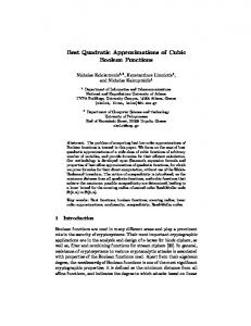
Figure 1: Level sets and critical points (a,b) of an input scalar function (m = 174, M = 180, s = 370) and its smoothed version achieved by applying the Tikhonov regularization without (c,d) (m = 44, M = 31, s = 91) and (e,f) with (m = 65, M = 23, s = 104) least-squares constraints. In both cases, the L∞ -approximation error is lower than 1%. Reb, black, and green points locate the m minima, M maxima, and s saddle points of the corresponding function.
with weights dij := kpj − pi k2 and fij := |f (pj ) − f (pi )|.
where jk+1 := j1 . For the definition of the lower link, we replace the inequality “>δ ” with “ δ implies Cδ ⊆ Cδ0 and the set {Cδ }δ gives a hierarchy of simplified critical points. Increasing δ, a larger number of critical points of f is simplified. In our implementation, the parameter δ is proportional to the maximum variation max(i,j) edge {|f (pi ) − f (pj )|} of the f -values along the edges of M. Note that the computational cost of the simplification procedure is O(n), where n is the number of vertices. Infact, we need to visit all the 1-stars of M and compare the f -values along their edges. Examples of simplification of the critical points are shown in Figure 2 and 3.
3. Simplifying the critical points of scalar functions In the following, we introduce a novel method to robustly classify and simplify the critical points of a function f : M → R. The idea behind our simplification of the critical points is to modify the definition in [2], which classifies the vertices of M on the base of the distribution of the f -values on their local neighborhoods. We propose to check the changes of the sign of f along the edges of the 1-star of each vertex with respect to a positive threshold δ. Indeed, the δ-sensitive sign of f along the oriented edge (pi , pj ) is defined as positive if f (pj ) − f (pi ) > δ; in this case, we write f (pj ) >δ f (pi ). Similarly, the δ-sensitive sign of f along the previous edge is considered as negative if f (pj ) − f (pi ) < −δ; hence, we write f (pj ) δ f (pi )},
This section describes two approaches to smooth a scalar function f through the properties of the Laplace-Beltrami operator (see Section 4.1). The first one uses the Tikhonov regularization to smooth arbitrary signals and treat all the function values with the same degree of importance (see Section 4.2).
and the (δ-sensitive) mixed link as Lk ± (i) := {jl ∈ Lk(i) : f (pjl+1 ) >δ f (pi ) >δ f (pjl ) or f (pjl+1 )