Computing Upper and Lower Bounds for the J−integral in Two ...

Computing Upper and Lower Bounds for the J−integral in Two-Dimensional Linear Elasticity Z.C. Xuan a 1 N. Par´es b J. Peraire c 2 a Department b Laboratori

of Computer Science, Tianjin University of Technology and Education, China

de C` alcul Num`eric, Universitat Polit`ecnica de Catalunya, Barcelona, Spain

c Department

of Aeronautics and Astronautics, Massachusetts Institute of Technology, USA

This paper is dedicated to the memory of Kwok Hong Lee

Abstract We present an a-posteriori method for computing rigorous upper and lower bounds for the J−integral in two dimensional linear elasticity. The J−integral, which is typically expressed as a contour integral, is recast as a quadratic continuous functional of the displacement involving only area integration. By expanding the quadratic output about an approximate finite element solution, the output is expressed as a known computable quantity plus linear and quadratic functionals of the solution error. The quadratic component is bounded by the energy norm of the error scaled by a continuity constant, which is determined explicitly. The linear component is expressed as an inner product of the errors in the displacement and in a computed adjoint solution, and bounded by an appropriate combination of the energy norms of the error in the displacement and the adjoint. Upper bounds for the energy norm of the error are obtained by using a complementary energy approach requiring the computation of equilibrated stress fields. The method is illustrated with two fracture problems in plane strain elasticity. An important feature of the method presented is that the computed bounds are rigorous with respect to the exact weak solution of the elasticity equations. 1

Previously at the Department of Mechanical Engineering, National University of Singapore, Singapore 2 Corresponding author : J. Peraire, Department of Aeronautics and Astronautics, Massachusetts Institute of Technology, 37-451, Cambridge, MA 02139, USA

Preprint submitted to Elsevier Science

21 December 2004

1

Introduction

The accurate prediction of stress intensity factors in crack tips is essential for assessing the strength and life of structures. A crack is assumed to be stable when the magnitude of the stress concentration at its tip is below a critical material dependent value. Stress intensity factors derived from linearly elastic solutions are widely used in the study of brittle fracture, fatigue, stress corrosion cracking, and to some extend for creep crack growth. Since the analytical methods for solving the equations of elasticity are limited to very simple cases, the finite element method is commonly used as the alternative to treat the more complicated cases. The methods for extracting stress intensity factors from computed displacement solutions fall into two categories: displacement matching methods, and energy based methods. In the first case, the form of the local solution is assumed, and the value of the displacement near crack tip is used to determine the magnitude of the coefficients in the asymptotic expansion. In the second case, the strength of the singular stress field is related to the energy released rate, i.e. the sensitivity of the total potential energy to the crack position. An expression for calculating the energy release rate in two dimensional cracks was given in [12] and is known as the J−integral. The J−integral is a path independent contour integral involving the projection of the material force derived from Eshelby’s [2] energy momentum tensor along the direction of the possible crack extension. An alternative form of the J−integral in which the contour integral is transformed into a domain integral involving a suitably defined weighting function is given in [5]. This alternative expression for the energy release rate appears to be very versatile and has an easier and more convenient generalization to three dimensions than the original form [12]. Regardless of the method chosen to evaluate the stress intensity factor, a good approximation to the solution of the linear elasticity equations is required. Unfortunately, the problems of interest involve singularities and this makes the task of computing accurate solutions difficult. For instance, it is well known [16] that the convergence rate of the energy norm of a standard finite element solution for a linear elasticity problem involving a 180o reentrant corner 1 is no higher than O(H 2 ), where H is the mesh size. This problem was soon realized and as a consequence, a number of mesh adaptive algorithms have been proposed. In some cases [6,7], the adaptivity is driven by errors in the energy norm of the solution, whereas in some others [3,4,13], a more sophisticated goal-oriented approach based on a linearized form of the output is used. Despite the improved accuracy generally afforded by the mesh adaptive algorithms, the computed energy release rates are still uncertain in that, it is very difficult to quantify, in absolute terms, the magnitude of the approximation errors. 2

In this paper, we present a method for computing strict upper and lower bounds for the value of the J−integral in two dimensional linear fracture mechanics. The method presented makes use of some previous results on implicit a-posteriori bounds for linear functional outputs of coercive partial differential equations [8,10,11]. Originally, these bounds were strict with respect to the output computed with a conservatively enriched finite element solution. More recently, these methods have been extended to produce bounds which are strict with respect to the exact weak solution of the partial differential equation [9,14,15]. The method presented involves no unknown constants or uncertain parameters and therefore the computed bounds are strict with respect to the exact weak solution of the underlying partial differential equation. The J-integral is written as a bounded quadratic functional of the displacement and expanded into computable quantities plus additional linear and quadratic terms in the error [17]. The linear terms are bounded using our previous work for linear functional outputs and the quadratic term is bounded by the energy norm of the error scaled by a suitably chosen continuity constant, which can be determined a priori. Moreover, the bound gap can be decomposed into a sum of positive elemental contributions thus naturally leading to an adaptive mesh adaptive approach [11]. We think that the algorithm presented is an attractive alternative to the existing methods as it guarantees the certainty of the computed bounds. This is particularly important in safety critical problems relating to structural failure. The method is illustrated for an open mode and a mixed mode crack examples.

2

Problem Formulation

We consider a linear elastic body occupying a polygonal region Ω ⊂ R2 where the boundary ∂Ω is composed of a Dirichlet portion ΓD , and a Neumann portion ΓN , i.e. ∂Ω = ΓD ∪ ΓN . For simplicity of presentation the Dirichlet boundary conditions are assumed to be homogeneous. The displacement field u = (u1 , u2 ) ∈ X ≡ {v = (v1 , v2 ) ∈ (H 1 (Ω))2 | v = 0 on ΓD } satisfies the weak form of the elasticity equations a(u, v) = (f , v) + hg, vi , in which

∀v ∈ X ,

Z

(f , v) =

Ω

(1)

Z

f · v dΩ ,

hg, vi =

ΓN

g · v dΓ ,

where f ∈ (H −1 (Ω))2 is the body force and g ∈ (H −1/2 (ΓN ))2 is the traction applied on the Neumann boundary. The bi-linear form a(w, v) : X × X → R is given by, Z

a(w, v) =

Z Ω

σ(w) : ε(v) dΩ =

3

Ω

ε(w) : C : ε(v) dΩ .

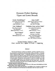
Here, ε(v) denotes the second order deformation tensor which is defined as the symmetric part of the gradient tensor ∇v. That is, ε(v) = (∇v + (∇v)T )/2. The stress σ(v) is related to the deformation tensor through a linear constitutive relation of the form σ(v) = C : ε(v), where C is the constant fourth-order elasticity tensor. It is well known that the solution, u, to the problem (1) minimizes the total potential energy functional Π(v) : X → R, 1 Π(v) = a(v, v) − (f , v) − hg, vi , 2 and that Π(u) = − 12 ||u||2 , where || · || = a(·, ·)1/2 denotes energy norm associated with the coercive bilinear form a(·, ·). In fracture mechanics we are often interested in determining the strength of the crack tip stress fields. A common way to do that is to relate the so called stress intensity factors to the energy released per unit length of crack advancement (see figure 1). If the total potential energy Π(u) decreases by an amount δΠ(u) when the crack advances by a distance δ` in its plane, we are interested in determining the energy release rate, J(u), such that, δΠ(u) = −J(u)δ` . For a two-dimensional linear elastic body the energy release rate, J(u), can x2 G

dl x1 Wc

Fig. 1. Crack geometry showing coordinate axes and the J−integral contour and domain of integration.

be calculated as a path independent line integral known as the J-integral [12]. If we consider the geometry shown in figure 1, the J-integral has the following expression, ! Z Ã ∂u e dΓ , J(u) = W n1 − T · ∂x1 Γ where Γ is any path beginning at the bottom crack face and ending at the top crack face, W e = (σ : ε)/2 is the strain energy density, T is the traction given as T = σ · n, and n = (n1 , n2 ) is the outward unit normal to Γ. An alternative expression for J(u) was proposed in [5], where the contour integral 4

is transformed to the following area integral expression, Z

J(u) =

Ωχ

Ã

∂χ ∂u − We (∇χ) · σ · ∂x1 ∂x1

!

dΩ .

(2)

Here, the weighting function χ is any function in H 1 (Ωχ ) that is equal to one at the crack tip and vanishes on Γ. For a given χ, J(u) is a bounded quadratic functional of u. For our bounding procedure it is convenient to make the quadratic dependence of J(u) more explicit. To this end, we define the bilinear form q¯(w, v) : X × X → R as, Z

Z ∂v 1 ∂χ q¯(w, v) = (∇χ) · σ(w) · dΩ − dΩ , σ(w) : ε(v) ∂x1 ∂x1 Ωχ Ωχ 2

and its symmetric part q(w, v) : X × X → R, q(w, v) = 21 (¯ q (w, v) + q¯(v, w)). It is clear from these definitions that, J(u) = q(u, u), and that there exists η < ∞ such that, |q(v, v)| ≤ η||v||2 , ∀v ∈ X . (3)

3

Bounding Procedure

Our objective is to compute upper and lower bounds for J(u), where u satisfies problem (1). We follow [17] and introduce a finite element approximation uH ∈ XH satisfying a(uH , v) = (f , v) + hg, vi ,

∀v ∈ XH .

(4)

Here, XH ⊂ X is a finite dimensional subspace of X. For simplicity, we shall assume that XH is the space of piecewise linear continuous functions defined over a triangulation, TH , of Ω which satisfies the Dirichlet boundary conditions. An approximation to J(u), JH , can be obtained as JH = q(uH , uH ), where, for convenience, χ in (2) is chosen to be piecewise linear over the elements TH ∈ TH . Exploiting the bi-linearity and symmetry of q(w, v), we can write J(u) − JH = q(u, u) − q(uH , uH ) = q(u − uH , u − uH ) + 2q(u, uH ) − 2q(uH , uH ) = q(e, e) + 2q(e, uH ) , where e = u − uH is the error in the approximation uH . It is clear that if we are able to bound the linear and quadratic terms by L± and Q, respectively, L− ≤ q(e, uH ) ≤ L+

and 5

|q(e, e)| ≤ Q ,

then, the bounds for J(u), J ± , follow as, J − ≡ JH − Q + 2L− ≤ J(u) ≤ JH + Q + 2L+ ≡ J + .

(5)

3.1 Linear term

In order to derive upper an lower bounds for the linear term q(e, uH ), we consider the following adjoint problem: find ψ ∈ X such that a(v, ψ) = q(v, uH ) ,

∀v ∈ X ,

(6)

and the corresponding finite element approximation, ψ H ∈ XH ⊂ X, such that a(v, ψ H ) = q(v, uH ) ,

∀v ∈ XH .

(7)

From (1) and (4), it follows that a(e, v) = 0 for all v ∈ XH . In particular, a(e, ψ H ) = 0. This, combined with the above equations (6) and (7) gives the following representation for the linear error term, q(e, uH ) = a(e, ψ) = a(e, ψ − ψ H ) = a(e, ²) , where ² = ψ − ψ H is the error in the adjoint solution. Now, using the parallelogram identity, we have that for all κ ∈ R+ , 1 1 1 1 a(e, ²) = ||κ e + ²||2 − ||κ e − ²||2 , 4 κ 4 κ and therefore, bounds for q(e, uH ) can be recovered as 1 1 1 1 1 1 1 1 ||κ e+ ²||2LB − ||κ e− ²||2UB ≤ q(e, uH ) ≤ ||κ e+ ²||2UB − ||κ e− ²||2LB , 4 κ 4 κ 4 κ 4 κ (8) where the subscripts U B and LB denote upper and lower bound, respectively. Strict upper bounds for ||κ e ± κ1 ²|| are found using the technique presented in [9] based on the use of the complementary energy principle. Here, the lower bounds are set to zero, that is ||κ e ± κ1 ²||LB = 0. We note that inexpensive methods for computing strict lower bounds are available and could be used to sharpen the results presented here (see [1], for instance). 6

3.2 Quadratic term In [17] it was shown that for two dimensional linear elasticity, a suitable value for the continuity constant in expression (3) is given by ηχ = max

TH ∈TH

s

µ

(3κ + 4µ)|∇χ|2

4 (3κ + µ) 3µ

³

´ ∂χ 2 ∂x1

+ (3κ + 4µ)

³

´ ∂χ 2 ∂x2

¶ ,

(9)

where µ = E/(2(1 + ν)) is the elastic shear modulus, κ is the elastic bulk modulus which is given by κ = E/(1 + 2ν)/(3(1 − ν 2 )) for plane stress, and κ = E/(3(1 − 2ν)) for plain strain. Here, E is the Young’s elastic modulus and ν is the Poisson’s ratio. The derivation of expression (9) is included in the appendix for completeness. Therefore, we write |q(e, e)| ≤ ηχ ||e||2 ,

(10)

and the computation of a bound for q(e, e) is straightforward once an upper bound for the error in the energy norm ||e|| has been obtained.

4

Computing Upper Bounds for the Energy

In this section, we give a brief description of the method employed for calculating upper bounds for the energy norm of the solution. A more detail presentation can be found in [9]. To this end, we consider the generalized problem: find z ∈ X such that a(z, v) = `∗ (v),

∀v ∈ X ,

(11)

and develop a procedure for calculating an upper bound for ||z||. It should be clear that if we set `∗ (v) ≡ κ ((f , v) + hg, vi − a(uH , v)) ±

1 (q(v, uH ) − a(v, ψ H )) , κ

(12)

then z ≡ κe ± ²/κ, as required in expression (8), whereas the choice `∗ (v) ≡ (f , v) + hg, vi − a(uH , v) ,

(13)

will give z ≡ e, as required in expression (10). We consider the space of symmetric second order stress tensors, S ≡ {σ ∈ (L2 (Ω))3×3 }, and introduce the symmetric positive definite bilinear form ac (τ , σ) : 7

S × S → R,

Z c

a (τ , σ) =

Ω

τ : C−1 : σ dΩ .

We note that if τ and σ are related to w ∈ X and v ∈ X, respectively, through the stress-strain relationships τ (w) = C : ε(w) and σ(v) = C : ε(v), then ac (τ (w), σ(v)) = a(w, v), for all w, v ∈ X. Further, we consider the subspace of equilibrated stress fields S eq ⊂ S defined as Z

S eq = {σ ∈ S |

Ω

σ : ε(v) dΩ = `∗ (v),

∀v ∈ X} .

(14)

The bounding result is based on the following Lemma: Lemma 1 Let z be the solution of (11). Then, for all σ ∈ S eq , we have ||z|| ≤ ac (σ, σ)1/2 .

PROOF. Let σ(z) = C : ε(z) then, Z

0≤ Z

=

Ω

(σ − σ(z)) : C−1 : (σ − σ(z)) dΩ Z −1

Ω

σ:C

: σ dΩ +

Ω

Z

σ(z) : ε(z) dΩ − 2

Ω

σ : ε(z) dΩ

= ac (σ, σ) + a(z, z) − 2`∗ (z) = ac (σ, σ) − a(z, z) . In the above expression, we have used the fact that, from (11), a(z, z) = `∗ (z). Adding −a(z, z) to both sides of the last expression above completes the proof. 2

Thus, we see that the problem of computing bounds for the energy norm of z reduces to determining stress fields in S eq . This is clearly a non-trivial task, but it turns out that the problem is greatly simplified if a domain decomposition strategy is adopted and the problem of determining global stress fields is reduced to that of determining equilibrated stress fields over each of the triangles of a mesh subject to some prescribed stress condition at the triangle boundaries. Here, we shall not consider this further and refer to [9] for a more detailed explanation including an explicit algorithm for constructing equilibrated stress fields by post-processing a finite element solution. The algorithm given in [9] applies to linear forcing functionals of the form `∗ (v) = (f ∗ , v) − a(z ∗ , v) +

X Z TH ∈TH

8

∂TH

λ∗ · v dΓ ,

(15)

where, the forcing data f ∗ and λ∗ and the displacement field z ∗ are piecewise polynomial functions. Further, the boundary of the computational domain is assumed to be represented by a collection of piecewise linear segments. Removing these restrictions seems feasible but effective algorithms for doing so are the subject of current research. Note that the linear forcing `∗ (·) associated with the primal error e given in equation (13) is already in the form of equation (15) provided that the forcing f and g are polynomial functions (take f ∗ ≡ f , z ∗ = uH and λ∗ = g ∗ in ΓN and λ∗ = 0 at the rest of the edges of the mesh). The linear forcing `∗ (·) associated with the errors κe ± ²/κ given in equation (12), on the other and, does not have the same form due to the term q(v, uH ). However, the term q(v, uH ) may be rewritten as Z

q(v, uH ) =

Ω

σ χ : ε(v) dΩ + (f χ , v) +

X Z TH ∈TH

∂TH

g χ · v dΓ ,

(16)

where ³ 1 ∂uH ´ 1 ∂χ σ χ = C : ∇χ ⊗ − σ(uH ) , 2 ∂x1 2 ∂x1

fχ = −

1 ∂((∇χ) · σ(uh )) , 2 ∂x1

and

1 g χ = (∇χ) · σ(uH ) n1 . 2 Note that if XH is the space of piecewise linear continuous functions over each triangle, then f χ ≡ 0 and the second term in (16) vanishes. The problem of determining an upper bound for the energy norm of κe ± ²/κ reduces to finding σ ∈ S verifying Z

X Z 1 1 1 (κg± g χ )·v dΓ, σ : ε(v) dΩ = (κf ± f χ , v)−a(κuH ± ψ H , v)+ κ κ κ Ω TH ∈TH ∂TH

where the right hand side is clearly in the form of equation (15) with f ∗ ≡ κf ± κ1 f χ , z ∗ ≡ κuH ± κ1 ψ H and λ∗ ≡ κg ± κ1 g χ . Finally, the upper bound for the energy norm is given by 1 1 1 ||κ e + ²||2UB = ac (σ ∓ σ χ , σ ∓ σ χ )1/2 . κ κ κ An attractive feature of the proposed approach is that the final expression for the bound gap, that is, the difference between the upper and lower bound, can be decomposed into the sum of positive elemental contributions. This leads naturally to an effective error estimation algorithm that can be used to adapt the grid in case the computed bounds are not considered to be sufficiently accurate. See [9–11,14,15] for further details. 9

5

Examples

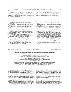
In this section, we present some numerical examples which illustrate the bound algorithm proposed for a plane strain problem under pure open mode and mixed mode loading. 5.1 Open Mode Example We consider a two dimensional rectangular section with two edge cracks subjected to a uniformly distributed tensile stress as shown in figure 2. The value of the tensile force acting on the two ends of the section is p = 1. The nondimensionalized Young’s modulus is 1.0 and the Poisson’s ratio is 0.3. p

5

60

5

5 Crack tip 30

5

Crack tip

20

p

Fig. 2. Geometry of a double edge-cracked section subjected to a uniform tensile stress (left) and support of weighting function χ for the evaluation of the J−integral (right).

Due to the symmetry of the problem, only one quarter of the domain is required for the analysis. We use a 5 by 5 square area surrounding the crack tip as the support, Ωχ , of the weighting function χ (see figure 2). Four estimates of J(u) are considered: the upper and lower bounds (J + and J − , respectively), their average, J ave = (J + +J − )/2, and also the output given by the finite element approximation, JH . An adaptive procedure has been used to reach a relative bound gap, (J + − J − )/(2J ave ), of less than 2%. Table 1 shows the results for the output JH , the computed upper and lower bounds, J ± , for J, and the relative bound gap for some of the intermediate meshes used in the adaptive procedure. Also, the first three linear finite element meshes of the adaptive procedure and the mesh for a 5% relative bound gap are shown in figure 3. It is worth noting that due to the very slow convergence of the 10

finite element solution, which is dominated by the singularity, it is crucial to use adaptive strategies to yield accurate bounds. Table 1 Bound results nel

416

525

759

1368

2962

10622

43733

JH

17.4156

18.5208

19.1307

19.3498

19.4601

19.5196

19.5369

J−

-27.7619

-2.7875

10.1176

15.1668

17.3981

18.6596

19.1712

J+

86.0779

49.2769

31.5315

24.9273

22.0868

20.5178

19.9343

J ave

29.158

23.245

20.825

20.047

19.742

19.589

19.553

1.952

1.110

0.514

0.243

0.119

0.047

0.0195

J + −J − 2J ave

(a)

(b)

(c)

(d)

Fig. 3. Finite element meshes: (a) coarse mesh nel = 416, (b) nel = 525, (c) nel = 759 and (d) mesh for a relative bound gap of 5%, nel = 10622.

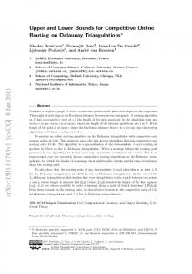
5.2 Mixed Mode Example Here, we consider a section with an inclined crack subjected to a uniformly distributed tensile stress as shown in figure 4. The value of the tensile force acting on the two ends of the domain is p = 1. The non-dimensionalized Young’s modulus is 1.0 and the Poisson’s ratio is 0.3. We use a 3 by 3 square area surrounding the crack tip as the support, Ωχ , of the weighting function χ (see figure 4). As in the previous example, an adaptive procedure has been used to reach the desired relative bound gap (J + − J − )/(2J ave ). Table 2 shows the results for the output JH , the computed upper and lower bounds, J ± , for J(u), and the relative bound gap for some of the steps of the adaptive procedure. Here, only 11

p

45

6

20

O

Crack tip

Crack tip 3

5 1.

Wc 3

10

5 1.

p

Fig. 4. Geometry of plate with an inclined crack subjected to a uniform tensile stress (left) and support of weighting function χ for the evaluation of the J−integral (right).

an accuracy of about 7% is obtained for J(u) in the finest mesh used. In order to determine the relative contributions of the linear and quadratic terms in expression (5), the bound gap, J + −J − , is written as J + −J − = 2Q+2L+ +2L− where 2Q and 2L+ + 2L− are the contributions due to the quadratic and linear error terms, respectively. Table 2 shows the bound for the quadratic term Q, its contribution to the relative bound gap Q/J ave and the percentage it represents of the total relative bound gap 2Q/(J + − J − ). We note that, for coarse meshes, the quadratic term represents the larger contribution to the bound gap, whereas for the more refined meshes, the larger contribution is due to the linear terms. Table 2 Bound results nel

164

302

632

1291

3231

8534

20217

41139

JH

4.601

5.528

6.043

6.261

6.405

6.469

6.492

6.501

J−

-32.079

-13.879

-4.130

0.961

3.958

5.273

5.829

6.079

J+

57.319

32.443

19.627

13.281

9.577

7.944

7.273

6.981

J ave

12.620

9.282

7.746

7.121

6.766

6.609

6.551

6.530

Q

29.292

14.168

6.785

3.320

1.316

0.511

0.215

0.104

Q/J ave

2.321

1.526

0.876

0.466

0.195

0.077

0.033

0.016

2Q J + −J −

66%

61%

57%

54%

47%

38%

30%

23%

J + −J − 2J ave

3.542

2.495

1.533

0.865

0.415

0.202

0.110

0.069

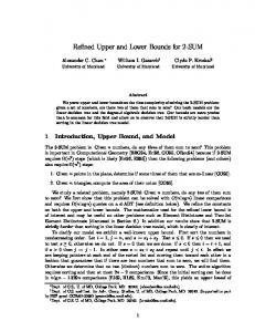
The first four meshes of the adaptive procedure as well as the final mesh are shown in figure 5. 12

(a)

(b)

(c)

(d)

(e)

J+ Jave J J(u)

50

Output bounds

40 30 20

Error in the Output bounds (positive)

Fig. 5. Finite element meshes: (a) coarse mesh nel = 164, (b) nel = 302, (c) nel = 632, (d) nel = 1291 and (e) final mesh nel = 41139.

4

2

10

10 0 -10

1

10

J+ J ave J

2

1 1

0

10

-20 -30 5000 10000 15000 20000 25000 30000 35000 40000

3

4

10 10 Number of elements

Number of elements

Fig. 6. Convergence of the upper and lower bounds J ± and the bound average J ave .

The convergence of the bounds J ± and the output estimate J ave versus the number of elements in the mesh are illustrated graphically in figure 6. Thanks to the mesh adaptive algorithm we are able to obtain an approximate convergence rate of one. This is certainly much faster than the convergence rate that would be obtained with uniform refinement. It is interesting to note, for comparison purposes, that if we were to consider a problem without singularities, a piecewise linear approximation will give, for uniform refinement, a convergence rate of one for the square of the energy norm of the error. Note that here, the convergence rate is measured with respect to the number of elements in the mesh and not the characteristic element size.

6

Conclusions

We have presented a procedure for the computation of upper and lower bounds for the exact value of the J−integral in linear fracture mechanics. To our 13

knowledge this is the first algorithm capable of computing such bounds for general geometries and general polynomial loading cases. Due to the presence of highly singular solutions, typical of fracture mechanics applications, finite element computations to estimate energy release rates exhibit very slow convergence rates. As a consequence, it is often difficult to determine, even in a heuristic manner, the magnitude of the errors in computed solutions. We feel that our approach is an important alternative to existing methods as it provides a certificate of accuracy with every computed solution. Given a finite element solution, the additional cost required to calculate the bounds is not significant as it only involves local operations.

Acknowledgments

We would like to acknowledge Professor K.H. Lee for introducing us to the subject of fracture mechanics and Professor A.T. Patera for our longstanding collaboration. Z.C. Xuan and J. Peraire would like to acknowledge the generous support for this research provided by the Singapore-MIT Alliance.

Appendix

Here, we prove expression (3) and provide an upper bound for the value of the constant η. In the two dimensional case, the stress and deformation tensors only have three independent components. Therefore, if we define the vectors σ = {σ11 , σ22 , σ12 }T and ε = {ε11 , ε22 , 2ε12 }T , we have that σ = Dε , where D is the matrix of elastic coefficients 



2 4  κ + 3µ κ − 3µ 0   





2 4 D=  ,  κ − 3µ κ + 3µ 0    0 0 µ

µ is the shear modulus and κ is the bulk modulus as defined in section 3. Let (

vx =

∂v1 ∂v2 ∂v1 ∂v2 , , , ∂x1 ∂x1 ∂x2 ∂x2 14

)T

,

then, for a given displacement field v ∈ X, we have, 



1 0 0 0  

 ε=  0 0 0 1  vx ,     0110 



2 µ 3 

4 µ 3

0 0 κ− κ+    σ =  κ − 23 µ 0 0 κ + 43 µ   vx ,    

(17)

1 1 ˜ W e = σ T · ε = v Tx D vx . 2 2

(18)

0

and ˜ is given by Here, D

µµ

0





2 4  κ + 3µ 0 0 κ − 3µ     0 µµ 0   

˜ = D    

0

µµ

0

κ − 23 µ 0 0 κ + 43 µ

 .    

The quadratic terms in (2) can now be expressed as (∇χ) · σ(v) · where

∂v 1 = v Tx Q v x , ∂x1 2





∂χ ∂χ ∂χ ∂χ 1 2 4  2(κ + 3 µ) ∂x1 (κ + 3 µ) ∂x2 µ ∂x2 (κ − 3 µ) ∂x1     ∂χ ∂χ ∂χ ∂χ  4 1 2µ ∂x µ (κ + µ)  (κ + 3 µ) ∂x2 ∂x1 3 ∂x2  1

Q=    

∂χ µ ∂x 2

∂χ µ ∂x 1

∂χ ∂χ (κ − 32 µ) ∂x (κ + 43 µ) ∂x 1 2

and

∂χ 1 W = v Tx ∂x1 2 Then, q(v, v) can be written as

(

e

0

0

0

0

)

∂χ ˜ D vx . ∂x1

"

#

∂χ ˜ 1Z v Tx Q − D v x dΩ , q(v, v) = 2 Ωχ ∂x1 and ||v||2 , is given by Z

a(v, v) =

Ω

˜ v x dΩ ≥ v Tx D

15

Z Ωχ

˜ v x dΩ . v Tx D

,    

If we consider now the symmetric generalized eigenvalue problem, Ã

!

∂χ ˜ ˜ vx = 0 , D − 2λD Q− ∂x1

(19)

it is clear that if we choose η = max{|λ1 |, |λ2 |, |λ3 |, |λ4 |} then, |q(v, v)| ≤ ηa(v, v) ,

(20)

as required. The eigenvalues of (19) can be found explicitly with the help of a symbolic manipulation program and the final expression for η is given in (9). We note that the value of η thus computed depends on ∇χ. In our context, χ is chosen to be piecewise linear on TH , in which case ∇χ is piecewise constant. In order to determine the appropriate value for η we simply take the maximum over all the elements in TH .

References [1] D´ıez, P., Par´es, N., and Huerta, A. Recovering lower bounds of the error postprocessing implicit residual a posteriori error estimates. International Journal for Numerical Methods in Engineering, 56 (10), 1465–1488, 2003. [2] Eshelby, J.D. The energy momentum tensor in continuum mechanics. Inelastic Behavior of Solids, vol. 77-114. McGraw-Hill, New York, 1970. [3] Heintz, P., and Samuelsson, K. On adaptive strategies and error control in fracture mechanics. Tech. rept. Preprint 2002-14. Chalmers Finite Element Center, Chalmers University of Technology, 2002. [4] Heintz, P., Larsson, F., Hansbo, P., and Runesson, K. Adaptive strategies and error control for computing material forces in fracture mechanics. Tech. rept. Preprint 2002-18. Chalmers Finite Element Center, Chalmers University of Technology, 2002. [5] Li, F.Z., Shih, C.F., and Needleman, A. A comparison of methods for calculating energy release rates. Engineering Fracture Mechanics, 21 (2), 405–421, 1985. [6] Lo, S.H., and Lee, C.K. Solving crack problems by an adaptive refinement procedure. Engineering Fracture Mechanics, 43 (2), 147–163, 1992. [7] Murthy, K.S.R.K., and Mukhopadhyay, M. Adaptive finite element analysis of mixed-mode fracture problems containing multiple crack-tips with an automatic mesh generator. International Journal of Fracture, 108 (3), 251–274, 2001. [8] Paraschivoiu, M., Peraire, J., and Patera, A.T. A posteriori finite element bounds for linear-functional outputs of elliptic partial differential equations. Computer Methods in Applied Mechanics and Engineering, 150 (1-4), 289–312, 1997.

16

[9] Pares, N., Bonet, J., Huerta, A., and Peraire, J. The computation of bounds for linear-functional outputs of weak solutions to the two-dimensional elasticity equations. Submitted to Computer Methods in Applied Mechanics and Engineering, 2004. [10] Patera, A.T., and Peraire, J. A general Lagrangian formulation for the computation of a-posteriori finite element bounds. Chapter in ”Error Estimation and Adaptive Discretization Methods in CFD”. Lecture Notes in Computational Science and Engineering, vol. 25, 2002. [11] Peraire, J., and Patera, A.T. Bounds for linear-functional outputs of coercive partial differential equations: Local indicators and adaptive refinement. In Proceedings of the Workshop On New Advances in Adaptive Computational Methods in Mechanics, edited by P. Ladeveze and J.T. Oden, Elsevier, 1997. [12] Rice, J.R. A path independent integral and approximate analysis of strain concentration by notches and cracks. Journal of Applied Mechanics, 35 (2), 379–386, 1968. [13] R¨ uter, M., and Stein, E. Goal-oriented a posteriori error estimates in elastic fracture mechanics. Fifth World Congress on Computational mechanics, Vienna, Austria, July, 2002. [14] Sauer-Budge A.M, Bonet J., Huerta A., Peraire J. Computing bounds for linear functionals of exact weak solutions to Poisson’s equation. Submitted to SIAM Journal on Numerical Analysis 2003. [15] Sauer-Budge A.M., Peraire J., Computing bounds for linear functionals of exact weak solutions to the advection-diffusion-reaction equation. Submitted to SIAM Journal on Scientific Computing 2003. [16] Szabo, B.A. Accuracy Estimates and Adaptive Refinements in Finite Element Computations. John Wiley. Chap. 3: Estimation and control of error based on p convergence, 1986 [17] Xuan, Z.C., Lee, K.H., Patera, A.T., and Peraire, J. Computing upper and lower bounds for the J-integral in two-dimensional linear elasticity. Presented at the SMA Symposium, National Univeristy of Singapore, Singapore, 2004

17