cesses is a key factor to increase the availability of the machine tool and achiev-
... Keywords: Condition monitoring, machine tool, machining process, milling,.
Condition Monitoring of Machine Tools and Machining Processes using Internal Sensor Signals
JARI REPO
Licentiate thesis Stockholm, Sweden, 2010
TRITA IIP 10-01 ISSN 1650-1888 ISBN 978-91-7415-600-3
School of Industrial Engineering and Management SE-100 44 Stockholm SWEDEN
Akademisk avhandling som med tillstånd av Kungliga Tekniska högskolan framlägges till offentlig granskning för avläggande av teknologie licentiatexamen i produktionsteknik fredagen den 9 april 2010 klockan 10.00 i sal M312, Kungl Tekniska högskolan, Brinellvägen 68, Stockholm. © Jari Repo, Mars 2010 Tryck: Universitetsservice US AB
Abstract Condition monitoring of critical machine tool components and machining processes is a key factor to increase the availability of the machine tool and achieving a more robust machining process. Failures in the machining process and machine tool components may also have negative effects on the final produced part. Instabilities in machining processes also shortens the life time of the cutting edges and machine tool. The condition monitoring system may utilise information from several sources to facilitate the detection of instabilities in the machining process. To avoid additional complexity to the machining system the use of internal sensors is considered. The focus in this thesis has been to investigate if information related to the machining process can be extracted directly from the internal sensors of the machine tool. The main contibutions of this work is a further understanding of the direct response from both linear and angular position encoders due the variations in the machining process. The analysis of the response from unbalance testing of turn tables and two types of milling processes, i.e. disc-milling and slotmilling, is presented. It is shown that operational frequencies, such as cutter frequency and tooth-passing frequency, can be extracted from both active and inactive machine axes, but the response from an active machine axis involves a more complex analysis. Various methods for the analysis of the responses in time domain, frequency domain and phase space are presented.
Keywords: Condition monitoring, machine tool, machining process, milling, position encoders, signal analysis
v
Acknowledgement The major part of the work presented in this thesis is carried out within the DLP-E project at Volvo Aero Corporation in Trollhättan, Sweden, during the years 2007-2009. The project was supported financially by VINNOVA1 through the MERA2 research programme, which is gratefully acknowledged. First of all, I would like to thank my local supervisor Dr. Tomas Beno and cosupervisor Prof. Lars Pejryd at the University West for their excellent guidance and encouragement during this work, even during the busiest periods. I also thank Prof. Mihai Nicolescu for giving me the opportunity to become a PhDstudent at the Royal Institute and for reviewing of this thesis. Project leader Andreas Rudqvist at Volvo Aero Corporation also deserves special thanks for his devoted participation in the project and for driving the project forward. During this work I have had the opportunity to use modern equipment at the Production Technology Centre in Trollhättan. Special thanks to Per Johansson, Tomas Gustavsson, Jörgen Berg, and Ulf Hulling, for your assistance during the experimental work. I also appreciate the support from my colleagues Mattias Ottosson and Hans Dahlin for solving some practical issues, and the support from Anna-Karin Christiansson. The discussions with Niklas Ericsson at the University West and Arne Nordmark at the Royal Institute of Technology also gave valuable guidance in some of the theory, which is gratefully appreciated. Finally, I would like to thank my family for supporting me in this work. Very special thanks to Linda and my children Robin and Ella for their patience and love throughout this journey. Jari Repo Trollhättan, Mars, 2010 1 2
The Swedish Governmental Agency for Innovation Systems Manufacturing Engineering Research Area
vii
Publications The following papers are appended to the thesis. Repo, J., Beno, T., Pejryd, L. (2009). New Aspects on Condition Monitoring of Machine Tools and Machining Processes. Proceedings of the 3’rd Swedish Production Symposium (SPS’09), Göteborg, Sweden, 2-3 December 2009. Repo, J., Beno, T., Pejryd, L. (2010). Machine Tool and Process Condition Monitoring Using Poincaré Maps. The International Conference on Competitive Manufacturing (COMA’10), Stellenbosch, South Africa, 3-5 February 2010.
ix
List of Symbols ap αL C(ε) d(ε) Δϕ(t) ftooth fz f0 Fs ϕ(t) ϕu (t) I(τ ) k λ1 m mu n ω N RL t Ts τ U Ua , Ub , Ur vc x = [x1 , x2 , . . . , xn ] x, y, z, S1 z z
Axial depth of cut [mm] Lissajous angle [rad] Correlation sum Correlation dimension Modulation signal [rad] Tooth-passing frequency [Hz] Feed per tooth [mm/tooth] Main frequency [Hz] Sampling frequency [Hz] Phase of an analytic signal [rad] Unwrapped phase [rad] Mutual information function Discrete time, signal segment index Largest Lyapunov exponent Embedding dimension Unbalance mass [kg] Spindle speed [rpm] Angular velocity [rad/s] Number of samples Lissajous radius [V] Continuous time [s] Sampling interval [s] Reconstruction delay Arbitrary voltage signal [V] Differentially measured voltage signals [V] Cutting speed [m/min] State vector Machine feed axis (x, y, z) and spindle axis (S1) Number of cutting inserts Complex/analytic signal
xi
Abbreviations ACF Autocorrelation function CBM Condition-based maintenance CMS Condition monitoring system CNC Computer numerical control DAC Digital-to-analogue converter DAQ Data acquisition DFT Discrete Fourier transform FAT Factory acceptance test FFT Fast Fourier transform FNN False nearest neighbour HHT Hilbert-Huang transform HT Hilbert transform IAT Installation acceptance test I/O Input/output MI Mutual information function RMS Root mean square SNR Signal-to-noise ratio TCM Tool mondition monitoring TCMS Tool condition monitoring system TFA Time-frequency analysis
xiii
Contents Abstract . . . . Acknowledgement Publications . . . List of Symbols . Abbreviations . .
. . . . .
. . . . .
. . . . .
. . . . .
. . . . .
. . . . .
. . . . .
. . . . .
. . . . .
. . . . .
. . . . .
. . . . .
. . . . .
. . . . .
. . . . .
. . . . .
. . . . .
. . . . .
. . . . .
. . . . .
. . . . .
. . . . .
. . . . .
. . . . .
. . . . .
. . . . .
. . . . .
. . . . .
. . . . .
v vii ix xi xiii
1 Introduction 1.1 Background . . . . . . . . . . . . . . . . . . . . . . . . . . . . 1.2 Aim and scope . . . . . . . . . . . . . . . . . . . . . . . . . . 1.3 Research approach . . . . . . . . . . . . . . . . . . . . . . . .
3 3 6 7
2 Principles of condition monitoring 2.1 Acceptance testing of machine tool components . . . . . . . . 2.2 Role of condition monitoring systems . . . . . . . . . . . . . . 2.3 Sensorless condition monitoring . . . . . . . . . . . . . . . . . 2.3.1 Internal drive signals . . . . . . . . . . . . . . . . . . . 2.3.2 Encoder signals . . . . . . . . . . . . . . . . . . . . . . 2.4 Position encoders in CNC machine tools . . . . . . . . . . . . 2.5 Principles for measuring of the position encoder output signals 2.5.1 Drive modules . . . . . . . . . . . . . . . . . . . . . . . 2.5.2 Counter card . . . . . . . . . . . . . . . . . . . . . . . 2.5.3 Data acquisition . . . . . . . . . . . . . . . . . . . . . .
9 9 11 13 13 14 14 16 16 17 18
3 Signal analysis methods 3.1 Characteristics of the output signals from position encoders for CNC machine tools . . . . . . . . . . . . . . . . . . . . . . . . 3.1.1 General considerations regarding the analysis of position encoder signals . . . . . . . . . . . . . . . . . . . . . . 3.1.2 Estimation of the SNR from measured signals . . . . .
19
I Introductory Chapters
19 23 24 xv
3.2 3.3
3.4
3.5 3.6
3.7
3.1.3 Filtering effects on the encoder signals . . . . . . . . . Fourier analysis . . . . . . . . . . . . . . . . . . . . . . . . . . Lissajous curves . . . . . . . . . . . . . . . . . . . . . . . . . . 3.3.1 Using Lissajous figures as vibration amplitude estimator 3.3.2 Formation of Lissajous figures from samples . . . . . . Hilbert transform . . . . . . . . . . . . . . . . . . . . . . . . . 3.4.1 Separation of the modulation signal from the unwrapped phase . . . . . . . . . . . . . . . . . . . . . . . . . . . . 3.4.2 Scaling of the unwrapped phase . . . . . . . . . . . . . Hilbert-Huang transform . . . . . . . . . . . . . . . . . . . . . Nonlinear time series analysis . . . . . . . . . . . . . . . . . . 3.6.1 Mutual information . . . . . . . . . . . . . . . . . . . . 3.6.2 Embedding dimension . . . . . . . . . . . . . . . . . . 3.6.3 Chaotic invariants . . . . . . . . . . . . . . . . . . . . . 3.6.4 Poincaré sections . . . . . . . . . . . . . . . . . . . . . Selection of signal analysis methods . . . . . . . . . . . . . . .
4 Exeperimental work 4.1 Linear encoder response to rotating unbalance . . . . . . . . . 4.1.1 Description . . . . . . . . . . . . . . . . . . . . . . . . 4.1.2 Signal analysis . . . . . . . . . . . . . . . . . . . . . . 4.1.3 Results . . . . . . . . . . . . . . . . . . . . . . . . . . . 4.2 Machining of aerospace component - industrial trial . . . . . . 4.2.1 Description . . . . . . . . . . . . . . . . . . . . . . . . 4.2.2 Segmentation of the measured signals . . . . . . . . . . 4.2.3 Vibration amplitude estimation from the Lissajous figure 4.2.4 Analysis of the rotary encoder signals . . . . . . . . . . 4.2.5 Phase space reconstruction . . . . . . . . . . . . . . . . 4.2.6 Results . . . . . . . . . . . . . . . . . . . . . . . . . . . 4.3 Slot-milling with various number of cutting inserts . . . . . . . 4.3.1 Description . . . . . . . . . . . . . . . . . . . . . . . . 4.3.2 Segmentation of the measured signals . . . . . . . . . . 4.3.3 Noise characterisation and SNR estimation . . . . . . . 4.3.4 Measuring of the Lissajous angle from the inactive feed axis signals . . . . . . . . . . . . . . . . . . . . . . . . 4.3.5 Spectral analysis . . . . . . . . . . . . . . . . . . . . . 4.3.6 Nonlinear analysis of the active feed axis modulation signal . . . . . . . . . . . . . . . . . . . . . . . . . . . 4.3.7 Phase plane analysis . . . . . . . . . . . . . . . . . . . 4.3.8 Results . . . . . . . . . . . . . . . . . . . . . . . . . . . xvi
25 26 27 27 31 32 35 36 36 37 38 38 39 41 43 47 47 47 49 53 54 54 55 57 58 60 65 67 67 70 71 72 73 75 78 79
5 Conclusions and future work 5.1 Conclusions of experimental work . . . . . . . . . . . . . . . .
83 84
References
87
MATLAB script est_alpha
91
II Included Papers New Aspects on Condition Monitoring of Machine Tools Machining Processes 1 Introduction . . . . . . . . . . . . . . . . . . . . . . . . . 2 Machine tool internal sensor signals . . . . . . . . . . . . 2.1 Linear and rotary encoders for motion control . . 2.2 Encoder output signals . . . . . . . . . . . . . . . 2.3 Additional information from the encoder signals . 3 Experimental setup . . . . . . . . . . . . . . . . . . . . . 3.1 Excitation of the machine tool structure . . . . . 3.2 Experiments with unbalance . . . . . . . . . . . . 3.3 Measurement setup . . . . . . . . . . . . . . . . . 4 Time series analysis . . . . . . . . . . . . . . . . . . . . . 4.1 Measured time signals . . . . . . . . . . . . . . . 4.2 Fourier analysis applied to the time series . . . . 4.3 Poincaré analysis applied to measured time series 5 Results and discussion . . . . . . . . . . . . . . . . . . . 6 Conclusions . . . . . . . . . . . . . . . . . . . . . . . . .
and . . . . . . . . . . . . . . .
. . . . . . . . . . . . . . .
. . . . . . . . . . . . . . .
99 100 101 102 102 103 103 103 104 105 105 105 105 106 109 110
References
113
Machine Tool and Process Condition Monitoring Using Poincaré Maps 1 Introduction . . . . . . . . . . . . . . . . . . . . . . . . . . . . 2 Theoretical framework . . . . . . . . . . . . . . . . . . . . . . 2.1 Dynamical systems . . . . . . . . . . . . . . . . . . . . 2.2 Phase space representation . . . . . . . . . . . . . . . . 2.3 Phase space reconstruction . . . . . . . . . . . . . . . . 2.4 Estimating the reconstruction delay . . . . . . . . . . . 2.5 Estimating the embedding dimension . . . . . . . . . . 2.6 Chaotic invariants . . . . . . . . . . . . . . . . . . . . . 2.7 Poincaré sections . . . . . . . . . . . . . . . . . . . . . 2.8 Visualising of Poincaré maps . . . . . . . . . . . . . . .
117 118 119 119 119 120 120 121 122 124 124 xvii
3
4 5
Experimental studies . . . . . . . . . . . 3.1 Preprocessing of the time series . 3.2 Reconstruction of the phase space Results and discussion . . . . . . . . . . Conclusions . . . . . . . . . . . . . . . .
References
xviii
. . . . .
. . . . .
. . . . .
. . . . .
. . . . .
. . . . .
. . . . .
. . . . .
. . . . .
. . . . .
. . . . .
. . . . .
125 125 127 128 128 131
Introductory Chapters
1
Chapter 1 Introduction 1.1
Background
Machine tools are composed of several subsystems, such as structures, electrical drive systems, controllers and actuators, which are all involved when performing the desired machining operations. The mechanical structure of the machine tool is often designed to be extremely rigid to withstand the forces created during the machining operation. Multitask machine tools are designed to perform several different machining operations such as turning, milling, drilling etc. in the same setup, which requires more degrees of freedom than dedicated machine tools. The additional number of degrees of freedom however, comes with a price - some of the rigidity is sacrificed. Multitask machine tools are not used for their rigidity, but for their capacity of handling large and geometrically advanced components and for their flexibility to allow manufacturing in a single setup, i.e. without the need of refixturing the component. The availability and utilisation of machine tools are key factors which have a direct influence on the economy of the manufacturing company. Non-working machine tools due to scheduled and unscheduled maintenance, process or machine tool component failure etc., have a negative effect on both availability and utilisation, which should be avoided as far as possible. The robustness of the machining process is also a key factor in reaching an economically favourable production simulation. 3
Machine tool structural components, such as guideways, bearings and ball screws, are subjected to gradual wear, which may be long-term. Testing of machine tool components on a regular basis is therefore important to reduce the risk of severe failures and breakdowns. Generally, the testing procedures require that the machine tool must temporarily be taken out of service, thus reducing the availability of the machine tool. The testing is often carried out as a part of maintenance programs, but testing may also be needed when failures, such as unexpected collisions, have occured. Maintenance of machine tools is important to ensure high consistency between the produced parts, especially when i) machine tools and spare parts are expensive ii) part consistency is critical iii) downtime cost is extremely high. Traditional methods to test different machine tool components include Double Ball-Bar (DBB), Laser Doppler Vibrometry (LDV) and Laser Interferometry. These methods require mounting of additional equipment to perform the measurements, which is relatively time consuming. Appropriate maintenance activities, i.e. corrective actions, are then undertaken based on the results from the measurements. It can however be questioned when to motivate the use of such detailed assessments of the machine tool because of the waste of valuable production time. The preferred way is to use quick test of some critical machine tool component to indicate if more advanced test methods must be used. The main drawback with the traditional methods for testing of machine tools is that these tests are performed off-process and are not considering the specific cutting parameters, and the spindle is not running. The positional accuracy of machine tools is dependent on the function of critical components, such as the guideways, ball screws, bearings and spindle shaft. Any deterioration, such as wear or misalignment, of these components, increases the risk of scrap production and later machine tool failures. Wear of spindle components has a strong influence on the performance of the spindle. Typical indicators of poor performance are i) increased temperature in the spindle housing due to wear of spindle bearings and ii) increased power consumption and iii) rotational asymmetry (run out) caused by misalignment of the spindle axis or iv) significantly increased vibration amplitudes. To increase the availability and utilisation of machine tools, a maintenance function based on the actual condition (or health) of the machine tools is therefore desirable. A condition monitoring system, CMS, capable of inprocess monitoring of the actual condition of the machine tool and machining process, may not only provide early indications of problems, but may also activate necessary control functions to perform the appropriate corrective ac4
tion, e.g. temporarily halting the machining process, updating the machining process parameters, or call for human assistance. This type of active control mechanism has a substantial potential to increase the robustness of the machining process. The aim with condition monitoring is early detection of disturbances in the machining process and wear of machine tool components. A machining system is the interaction between the between the machining process and the elastic structure of the machine tool. The cutting forces are created through the interaction between the cutting tool and the workpiece. Tool wear has been excessively researched in the past and have focused on tool wear detection, tool breakage detection, and the estimation of remaining tool life. Various techniques have been applied, with and without additional sensors. Sensor based tool condition monitoring, TCM, are mainly based on measuring of the cutting force components using a multi-channel table dynamometer or rotating dynamometer, vibration amplitude using multi-channel accelerometers, audible sound from the machining process, and high-frequency sound or acoustic emission, AE. Sensorless TCM are mainly based on measuring of internal drive signals, such as the feed motor current, spindle motor current and spindle power. Combined measuring of multiple quantities is also possible. The use of external sensors is however not always practical since it adds complexity to the overall machining arrangement - various number and types of sensors must be mounted in the close vicinity of the machining process, making them subjected to the heat, chips and coolant, which may affect the lifetime of the sensors and also quality of the measurements. The wirering of the sensors is another issue that must be considered especially in more advanced machining operations. External sensors also require additional maintenance and calibration in order to function properly. A potentially attractive way to achieve a more robust solution to condition monitoring, compared with the traditional approach using external sensors, is to use the internal sensors and signals which are already available in the machine tool. Assuming that more information which is relevant to the monitoring task actually can be extracted from the signals, the complexity of the monitoring system may therefore be significantly reduced. Finding signatures of specific phenomena, such as disturbances due to wear of critical machine tool components, and disturbance in the machining process due to tool wear or breakage, may also provide deeper insight into the health of machine tools 5
and further understanding about the dynamics of machining processes due to the choice of machining parameters. The information can then be used at higher level to support a condition based maintenance, CBM, function within the manufacturing company. An issue often experienced in larger manufacturing companies with machine parks comprising multiple machine tools built on the same specification is that even if these machine tools are expected to produce identical parts, there may be some deviations in the dimensions of the produced parts, i.e. machine tools sometimes appear to behave more like individuals. This is detected after a dimensional check of the produced part and additional rework may be needed to achieve the desired dimensions. Very often it is not always possible with the currently used test methods to pin point the root cause of the problem. In general, this has a negative effect on the productivity in that special versions of the numerical code and compensation schemes must be developed and maintained for each of the supposedly identical machine tools. This additional complexity with variations among machine tools is however left outside this thesis.
1.2
Aim and scope
The aim of this work is to investigate the possibilities to use internal machine tool signals for condition monitoring of machine tools and machining processes. This is important in order to achieve more robust machining processes without adding complexity to the overall machining system. In this work, a 5-axis multitask machine and various material removal processes, such as milling and drilling, are considered. Condition monitoring involves measuring, processing and analysis of signals, the characterics of the measured signals must be known in order to select appropriate methods for the processing and analysis of them. A major part in this work is therefore to study the responses during various type of excitations of the machine tool and present suitable strategies to extract the useful part from the signals. The main research question is therefore whether it is possible to extract useful information related to the health of the machine tool and stability of machining processes from the internal sensors of the machine tool. A related question is 6
also are what type of phenoma can actually be detected. The quality of the information can be expressed in terms of its objectivity, repeatability, accuracy and errors, which must must also be considered in order to evaluated the usefulness of the extracted information from the point of view of machine tool availability. The sensitivity of the method is related to the minimum detectable change of the wear and level of disturbance, which needs to be investigated. The research questions for this thesis can be summarised as:
• Is it possible to detect deficient machine tool components using internal sensor signals? • Is it possible to detect machining process instabilities using internal sensor signals? • What signal analysis methods are suitable to extract the useful part from the internal sensors signals?
1.3
Research approach
The thesis has taken an experimental approach and is based on observations obtained during machining in a modern 5-axis multitask machine tool. Various experiments have been performed which allow the systemtic study of certain phenomena. The main focus has been to study the time behaviour of the output signals due to vibration generated for various periodic excitation and vibration generated from rotating unbalance and vibrations generated from impacts. The characteristic behaviour of the encoder output signals was initially unknown and needed a thorough investigation before any further analysis of them could be undertaken. To get a fundamental understanding of the behaviour of the signals, initial experiments with minimal complexity have been carried out, including both non-machining and various machining tests. Several possibilities for the connection of the measurement equipment have been tried 7
out until a final measurement chain were developed which allows high-quality and reliable measurements without disturbing the overall machining system. Various numerical methods have been applied to the encoder signals in order to extract the useful part from the signals. A subset of these methods have then been selected when characterising various machining processes. The analysis has been carried out offline.
8
Chapter 2 Principles of condition monitoring Maintaining the health of macine tools and establishing stable machining processes is of major importance to reduce the risk of malfunctioning equipment and ensure that high quality parts are produced. This can be achieved by testing of critical machine tool components and online measuring and analysis of one or more quantities from the machining process in order to adjust the process towards more stable machining regions. From the initial acceptance tests of machine tools this chapter reviews some principles of condition monitoring of the machining process using various methods found in the literature.
2.1
Acceptance testing of machine tool components
Testing of machine tool components is important through its life cycle to avoid severe breakdowns during operation. The testing procedure itself is carried out both at the suppliers shop and after the installation. Generally, a factory acceptance test, FAT, is carried out first at the suppliers shop before the delivery of the machine tool. After installation at the customers shop, an installation acceptance test, IAT, is performed as a final validation. Rearrangement of machine parks at the customers shop, which may affect the alignment of structural components, is another reason when acceptance tests should be performed. For a 5-axis multitask machine tool, the acceptance test procedure may include measuring of the following properties [1]: 9
• noise level during a well-defined and well-behaved machining operation, • geometrical measurement, • spindle speed, • feed rate, • idling power, • radial and axial spindle vibrations (full spindle speed range), • deflection of the machine tool structure, • clamping force, i.e. the force that pulls the tool into the tool holder, and • position accuracy of the linear and rotary axes The duration of the FAT and IAT depends on the complexity of the machine tool and which properties are measured, but may take several days to complete. These tests are however performed only a few times during the life cycle of the machine tool. The linear and angular position axes are tested for positional accuracy, repeatability and backlash. Measuring of the alignment of the linear axes is normally performed using LASER interferometry. The accuracy of the spindle shaft speed is measured using rotary encoder. The linear and circular interpolation capability of the machine tool is also measured to obtain the maximum deviation from the programmed motion. The circularity test is normally performed using special measuring devices, such as the Renishaw™ Double Ball Bar, DBB. Machining of high quality parts is strongly dependent on that high relative position accuracy between the workpiece being machined and the cutting tool can be achieved by the machine tool. The machine tool structure will however deform over time due to thermal effects and wear of structural components, which makes the long-term behaviour of the machine tool difficult to predict. Deterioration of the machine tool condition may also affect its positional accuracy. Thus, failing in maintaining the positional accuracy may result in that the dimensions of the produced part will fall outside the part specification. The manufacturing company may therefore not entirely rely on initial acceptance tests, ATs, since the results from ATs will most probably only be valid within a limited time window. 10
2.2
Role of condition monitoring systems
The machining process is either continuous, such as turning or drilling, or intermittent, such as the milling operation. Continuous operations are performed with single cutting edge, removing material from one spindle revolution to the next. Intermittent operations involve one or more cutting edges, removing material from one tooth to the other. In both cases, material is removed from the workpiece under the generation of chips. The machining operations are controlled by various parameters, such as the spindle speed, depth of cut and feed rate, etc. If the correct machining parameters are set, the machining operation is expected to perform well and the final produced part will meet the final requirements given in the part specification. Depending on the machining process characteristics, the cutting tool may have a short or long life time. For cost effective production, the number of tool changes should be kept at minimum and the cutting tool inserts must be used close to the limiting tool life without violating the overall machining system. This requires in-depth knowledge about the tool wear rate and maximim tool life for the actual machining setup and machining conditions. In well behaved machining processes, the tool life can be more or less accurately determined and the tool change interval may therefore be optimised using some tool wear criterion, such as the maximum flank wear. The simple case will however require almost a gradual tool wear. For more complex materials and demanding machining processes, tool wear may become excessive and sudden events, such as tool chipping and breakage, will most likely occur. The monitoring of the tool condition may therefore be very difficult since such unexpected events occur within a relatively short time interval. The behaviour of the machining process is also dependent on the workpiece material, cutting tool material and geometry, actual machining process parameters and the condition of the overall machining system. Hardness variations in the workpiece material, which can be traced back to the manufacturing of the workpiece material itself, is another factor which may increase the unpredictability of the machining process, leading to drastically shorter tool life, tool chipping and tool breakage. The cutting tool can be regarded as the limiting component of the machining process and is the main reason why machining process condition monitoring 11
Figure 2.1 – Role of condition monitoring systems.
is mostly concerned with the actual state of the cutting tool. When the cutting tool is worn the cutting force and vibration amplitudes tend to increase and the machining process may become unstable. The main task of the condition monitoring system, CMS, is to collect relevant data from the machining process, then process and analyse the data to detect symptoms of troubles, but also to signal a control function to adjust the machining process parameters to a more stable machining region. Within the stable region, optimisation can be performed to meet some criterion, such as maximising the material removal rate, minimising the production cost, etc., see Figure 2.1. Process instabilities are often recognised as increased vibration amplitudes, which may cause unexpected events such as tool failures, which can be harmful to the workpiece and machine tool. To meet the increasing demands on higher productivity and high quality of the produced parts, vast amount of research has been invested in the development of CMSs in order to prevent failures and compensate for faults. A various number of sensors have been used for the monitoring of the state of the cutting tool. A review on the use of external sensors for monitoring of the state of the cutting tool has been presented by Byrne et al. [2]. The difficulties in designing reliable TCMs can be related to the complexity of the machining process itself, which may have one or more of the following characteristics, apart from the changes of the machine tool itself [3]: 12
1. complex to chaotic behaviour due to non-homogeneities in workpiece material, 2. sensitivity of the process parameters to cutting conditions, and 3. nonlinear relationship of the process parameters to tool wear.
2.3
Sensorless condition monitoring
Sensorless condition monitoring is about monitoring of the machining process by utilising the existing sensors and signals in the machine tool without using external sensors, such as force sensors and accelerometers. The main advantage is that the additional complexity is kept to a minimum while reducing the cost of the condition monitoing system. Two types of internal signals are considered, i.e. internal drive signals and encoder signals.
2.3.1
Internal drive signals
Internal drive signals, such as the spindle motor current and feed drive current, can be measured with a non-intrusive Hall effect sensor [4]. Measuring of the current signal from the servo drive motors and spindle motors has been widely used as a means of indirect measuring of the cutting force to avoid the impracticability of force dynamometers. However, the observed current signal from the servo drive motor contains additional components related to acceleration and deceleration of the work table, friction force in the guide way, feed direction change, etc. Thus, to obtain a reliable estimation of the cutting force, the undesired components in the current signals must first be removed, which can be accomplished using special pre-processing methods. The cutting force estimation method presented by Kim et al. [5] also makes use of the internal feed rate signals to generalise the cutting force estimation to multi-axis machining. [6] utilised the spindle power consumption signal and feed drive current signals to estimate tool wear in high-speed milling. Internal signals may also be accessed directly from diagnostics sockets (DAC outputs) on the drive modules. However, these signals may have limited use due to the relatively low internal sampling rate (a few milliseconds) and distortions due to internal digital-to-analogue conversion. The internal sensor may 13
also be located far away from the component to be monitored. Internal drive signals also represent a sum of signals originating from different sources [7]. From a condition monitoring point of view, the use of the internal drive signals may be inappropriate due to the relatively low sampling rate and internal delays, which in turn may result in poor and incorrect results and assumptions. A TCM system that utilises the existing spindle speed and spindle load signals have been reported by Amer et al. [8].
2.3.2
Encoder signals
The machine tool manufacturer have several options to achieve high position accuracy. The most popular way is to use position encoders due to their high reliability and sensitivity. Linear and angular position encoders are integral parts of the machine tool and used internally to close the position control loops. These encoders measure the position along the feed axes rotating axes (spindle and turn table) respectively. Encoders have been used in the past research. Kaye et al. [9] used the change in spindle speed (measured with an optical encoder) to detect tool wear in turning. Jang et al. [10] used the pulse signal from a rotary encoder to perform once-per-revolution sampling of the vibration signal. Plapper and Weck [7] found that backlash in the drive chain manifests itself as an increased difference between the position from the motor encoder and the encoder of the direct position when the axis movement is reversed. Verl et al. [11] used the output signals from the position encoders to quantify the wear of the ball screw drive. They concluded that the accuracy of positioning is a key factor to initiate maintenance. Klocke et al. [12] took a step towards position-oriented process monitoring by utilising all position encoder signals from a 5-axis milling machine for an in-depth analysis of a freeform milling operation. A complete measurement chain was also presented, allowing synchronisation of the position signals with other type of signals, such as cutting force and vibration signals.
2.4
Position encoders in CNC machine tools
Various types of position encoders are available, such as linear or rotary encoders. The encoder may be either an absolute or an incremental encoders. Encoders are also based on different physical principles, such as light, mag14
netism or induction. Rotary encoders are mounted directly on the motor shaft to measure the angular position and linear encoders are mounted on along the feed axes, which gives a direct measuring of the position. Linear position can also be measured indirectly using a rotary encoder on the driving shaft. In the latter case the pitch of the lead screw must be known to get the position. For high precision measuring of the position using encoders the direct measuring principle is prefered.
Figure 2.2 – Internal position encoders on a 5-axis multitask machine tool (DECKEL MAHO). The 5-axis multitask machine tool1 used in the experimental work in this thesis, is equipped with an rotary encoder2 to measure the angular position of the spindle shaft and turn tables, and linear encoders3 to measure the position along the feed axes. The physical structure of the 5-axis multitask machine tool and available position encoders is illustrated in Figure 2.2. The position accuracy of machine tools is strongly dependent on the type of position encoders used. Modern machine tools are equipped with so called Sin/Cos-encoders, which give continuous sinusoidal outputs instead of square waves as is the case for incremental optical encoders. Position estimation from the signals is mainly based on interpolation. The main advantage with continuous output signals is that the signals may be interpolated to an arbitrary resolution to achieve the desired accuracy. 1
DMU/DMC 160 FD WOELKE MINI-Sensor WG 05 3 HEIDENHAIN LC 481 2
15
2.5
2.5.1
Principles for measuring of the position encoder output signals Drive modules
The position encoders are initially connected to the drive modules of the machine tool as shown in Figure 2.3. The drive modules have special interpolation circuits to calculate the position along the machine axis using the encoder output signals. For the connection of the encoder output signals to an external measurement system, direct measuring of the continuous output signals is considered in order to obtain as clean signals as possible.
Figure 2.3 – Drive modules in the DMU/DMC 160 FD machine tool.
Two options for the measuring of the encoder output signals are considered. One is the use of an external counter card, second is the use of traditional data acquisition, DAQ. A brief description of these measurement systems is given in the following subsections. 16
2.5.2
Counter card
The first option is to connect the encoder signals to an external counter card, such as HEIDENHAIN IK 220 [13]. This card is used for special purpose measuring of both angular and linear position and allows measuring of two motion axes simultaneously. The card is also compatible with various signal interfaces, such as 1Vpp signals. The input signals for each motion axis are encoder output signals ±A and ±B. To avoid damage to the original cables and signals, breakout boards4 is used, from where the selected signals easily can be identified and connected to the IK 220 board, see Figure 2.4.
Figure 2.4 – Measurement chain using the IK 220 counter card. However, there is an issue with a disturbance on the control system when the measurement computer is powered on when encoder signals are connected to the IK 220 board. This is probably caused by an input impedance change detected by the drive module. The machine tool will end up in a faulty state and will be unable to operate. A complete restart of the machine tool may be required to resolve the problem. To avoid such problems the encoder signals may only be connected to the IK 220 board during measuring, which of course is very inflexible. To overcome this issue, the drive modules must be isolated from the measurement system. The simplest solution is to add a switch mechanism between the encoder signals and the IK 220 board. The switch can either be constructed using operational amplifiers which provide nearly infinite input impedance, or using a manually controlled on-off button to control a set of relay coils to connect and disconnect the signals. A better solution to guarantee safe operation is to supplement the measurement chain with opto-couplers in order to isolate the measuring system from the drive modules. 4
BRK15MF and BRK25MF from Winford Engineering
17
The IK 220 interpolation card has been tested for calculation of the angular position of the spindle shaft. The card was configured to sample every 100 μs (10 kHz), which is the maximum sampling rate of the counter card. For monitoring of the encoder output signals at higher spindle speeds and feed rates, the 10 kHz sampling rate may be insufficient. According to Eq. 3.1 and Eq. 3.2, a Nyqvist frequency of 5 kHz (half of the maximum sampling frequency) allows measuring of spindle speeds up to 1171 rpm and feed rates up to 6000 mm/min. Furthermore, the size of the internal circular buffer in the IK 220 card used to store the counter values is limited to only 8191 positions, resulting in a buffer overflow if the measuring takes longer than 0.8191 seconds. To make longer recordings possible, the data from the IK 220 buffer must be read into the PC RAM during measuring.
2.5.3
Data acquisition
The second option for measuring of the encoder output signals, is to differentially measure the encoder signals ±A, ±B, ±R using multi-channel digitial input modules, see Figure 2.5. This is the preferred option since it allows simultaneous measuring of all machine axes. This also offers higher flexibility when setting the sampling rate. Selecting an appropriate sampling rate is critical to obtain a good digital representation of the measured signals. The digital input module NI 9402 (4-ch/16-bit/100kHz) is used in the experimental work. The maximum Nyqvist frequency of the measured signals is 50 kHz, allowing measuring using a wider range of spindle speeds and feed rates.
Figure 2.5 – Measurement chain using a digital input module.
18
Chapter 3 Signal analysis methods This chapter presents an overview of signal analysis methods applicable to the output signals from the position encoders described in Section 3.1. Both traditional linear methods and more advanced methods are presented. There are also some general considerations related to filtering of the encoder signals. Some of the methods will be used in the experimental work presented in the next chapter in order to characterise and analyse the operational conditions of machining processes where analysis in the time domain, frequency domain and phase space are considered.
3.1
Characteristics of the output signals from position encoders for CNC machine tools
The choice of appropriate methods for signal processing and signal analysis is mainly based on the characteristics of the measured signals and of course also on the nature of the phenomena being investigated. This section therefore presents the most important characteristics of the output signals from both rotary encoders and linear encoders. Generally, the Sin/Cos-encoders for the linear and angular motion axes provide the differential continuous position signals ±A and ±B which are 90 degree out of phase, also known as quadrature signals. The angular position encoder also provides the reference mark signal ±R which provides a pulse to indicate 19
a full revolution of the rotating axis being measured. The signal denoted with a minus (−) sign is basically the inverse of the signal denoted with a plus (+) sign and is a well known technique used especially in harsch industrial environments where the signals may be prone to various distrubances, such as impulsive noise originating from electrical discharges or due to other type of environmental noise. The basic idea is that the noise component will show up in both signals and can thus be easily removed by applying the differential measurement principle on the signals [14]. In the continuation of this text, the differentially measured signals are denoted Ua , Ub and Ur . These signals are used by the drive modules to determine the position along the motion axis but also to determine the direction of motion. In the positive motion direction, the signal Ua is ahead of Ub and vice versa when moving in the negative direction.
Amplitude
The differentially measured output signals from the rotary encoder are the two continuous 1Vpp signals Ua and Ub . As already mentioned, there is also a reference mark signal Ur available from the rotary encoder which gives a pulse after each full spindle revolution, see Figure 3.1.
T ime Figure 3.1 – Typical rotary encoder signals Ua , Ub and Ur . The rotary encoder signals are used internally by the machine tool drive modules to determine both the angular position of the rotating axis and the direction of motion. The main frequency in the rotary encoder signals Ua and Ub is related to the actual spindle speed. When the spindle speed is near constant or steady state, the output signals will be near sinusoidal with 256 cycles per spindle revolution. The relation between the steady state spindle speed n [rpm] and the main frequency f0 in the output signals is given as f0 =
n · 256 [Hz] 60
(3.1)
From Eq. 3.1 it can be noted that the main frequency in the output signals becomes relatively high even for relatively low spindle speeds, see tabulated 20
Table 3.1 – Main frequency f0 for some spindle speeds n. n [rpm] f0 [Hz] 100 427 500 2133 1000 4267 5000 21333 10000 42667 values in Table 3.1. The output signals from the linear encoders are the two 1Vpp signals Ua and Ub . The encoder signals are used internally by the drive modules to determine the direction of the motion and the actual position relative to the machine coordinate system. The type of response from the linear encoder depends on whether the signal is measured from an active or inactive machine axis. In this context, an active machine axis is a part of either a linear (feed axis) or angular (main spindle or turn table) motion. This motion itself can be either steady state motion, i.e. constant velocity, or time-varying. An inactive machine axis is regarded to be in a ”hold state” and not activly controlled to a specific location.
Amplitude
Figure 3.2 shows a typical response from an inactive feed axis during an intermittent machining operation. The response is obviously nonlinear and periodic.
T ime Figure 3.2 – Typical encoder output signals Ua , Ub from an inactive feed axis during an intermittent machining operation, here plotted with the spindle reference mark signal Ur .
Figure 3.3 shows a typical response from an active feed axis during an intermittent machining operation. In this case the response is obviously nearsinusoidal. 21
Amplitude
T ime Figure 3.3 – Typical encoder output signals Ua , Ub for an active feed axis during an intermittent machining operation.
The main frequency f0 in the linear encoder output signals for an active feed axis is directly related to the actual feed rate f and given as f0 =
f 1.2
[Hz]
(3.2)
where f denotes the steady state feed rate [mm/min]. Both Eq. 3.1 and Eq. 3.2 have been found empirically by measuring the main frequency in the position signals Ua and Ub from the main spindle and feed axes for steady state spindle speeds and feed rates and performing the FFT on the measured 1 in Eq. 3.2 can be found by performing a signals. The proptionality constant 1.2 least squares linear fit of the feed rates (1000, 1500, . . . , 5000) mm/min and the corresponding frequencies found by performing a spectral analysis. The value of the proportionality constant may vary between different encoder types and their resolution since it includes the number of cycles per millimeter movement. The equivalence of Eq. 3.2 can be written as f0 =
f · 50 [Hz] 60
(3.3)
which shows the number of cycles of the sinusoid per mm movement, which is 50 cycles/mm for the linear encoder in use. According to the linear encoder data sheet1 , one period of the output signals from the linear encoder corresponds to a relative linear movement of 20 ± 3μm, which is in agreement with Eq. 3.3. Notice that the relations in Eq. 3.1 and Eq. 3.3 only apply for active machine axes and give the main frequency for constant spindle speed and feed rate respectively. 1
22
HEIDENHAIN, Position Encoders for Servo Drives, 12/2001
For multi-tooth cutters with z cutting edges, such as milling tools, the feed rate f is given as f = fz · z · n [mm/min]
(3.4)
where n is the spindle speed [rpm] and fz denotes the feed per tooth [mm/tooth]. An important operational frequency is the tooth-passing frequency defined as the inverse of the time between two subsequent tooth-passes. For a multitooth cutter with z teeth and uniform angular spacing between the individual cutting inserts, the tooth-passing frequency is defined as ftooth =
3.1.1
n ·z 60
[Hz]
(3.5)
General considerations regarding the analysis of position encoder signals
Some difficulties may be encountered in the analysis of position encoder signals. 1. For active machine axes, the frequencies in the measured signals are not initially related to any operational frequencies, why a transformation of the signals is needed in order to facilitate the extraction of the relevant information from the signals. 2. For inactive machine axes, the disturbances affect both the frequency and amplitude of the signals. The operational frequencies may be therefore found directly in the signals but the interpretation of the timevarying amplitude may be difficult due to the fact that encoder signals in general are amplitudelimited, i.e. 1Vpp signals. 3. In the general machining case, it is most likely that the operational frequencies will be time-varying due to variations of the spindle speed and feed rate or various processrelated disturbances. Thus, in order to use the output signals from position encoders as the input for condition monitoring, constant speed and feed rates cannot be assumed. 4. For active machine axes, the main frequency in the signals acts as a carrier component, which will be modulated due various disturbances in 23
the machining process. The useful information is then available in the frequency of the signals as a modulation signal. In order to analyse the process dynamics from the signal, the modulation signal must be separated from the signal, i.e. signal must be demodulated. Once removed, the modulation signal can be analysed. This may however be difficult in the case when the carrier component is time-varying as in the general machining case. 5. Noise-free signals do not exist in the real world, especially not in harsch industrial environments, why a characterisation of the noise by means of its probability distribution may be useful. A quantitive measure is the signal-to-noise ratio (SNR) which is useful when evaluating the amount and quality of the information content in the signal.
Furthermore, in the general machining case, the number of simultaneous active feed axes will vary and the response from the individual feed axes may also be different due to varying rigidity of the machine axes. To reduce the complexity of the signal analysis due the aforementioned factors, the response from single-axis2 machinining operations has therefore been considered in the experimental work presented in Chapter 4.
3.1.2
Estimation of the SNR from measured signals
Any given measured signal is composed of two components, one is the useful and meaningful signal s(t) and the other is the undesired noise signal v(t). The measured signal is then given as the sum s(t) + v(t). One measure used to quantify how much the signal s(t) is correpted by the noise v(t) is the signal-to-noise ratio, SNR, defined as the ratio between the signal power Ps and the noise power Pv and is often expressed in dB. A definition of SNR which takes into account the presence of the noise, is given as [15] �
SNRdB = 10 log10
Ps + Pv Pv
�
�
= 10 log10
Ps +1 Pv
�
(3.6)
which assumes that the noise can be measured by having the signal disconnected. The other problem is that often the power in the signal and noise is determined by measuring the voltage with and without the signal. If the 2
24
a single active feed axis with the spindle running
voltages are measured as true RMS-values, then the power values in Eq. 3.6 can be replaced with the square of the RMS-values [15] �
SNRdB = 10 log10
(srms + vrms )2 2 vrms
�
�
= 20 log10
srms +1 vrms
�
(3.7)
Notice that in Eq. 3.7 it has been assumed that the signal and noise are uncor2 related, why (srms + vrms )2 = s2rms + vrms since the double product, 2srms vrms , is zero. The error in the estimation of SNR will be small if Ps /Pv is large. The size of the error also depends on whether the power or RMS values have been measured. In practice, if the true RMS values are measured and the estimated RMS values must be corrected [15].
s(t)+v(t) [V]
Figure 3.4 shows 2000 voltage samples of a noise signal and a disturbed signal (with their mean value removed) recorded at 1024 Hz from the y-axis encoder of the machine tool.
v(t) [V]
0.01 0 −0.01
0.2 0 −0.2
t
t
Figure 3.4 – Recorded noise signal (left) and noise-contamined signal (right) with their mean values removed. In the case�of N voltage samples {u1 , u2 , . . . , uN }, the RMS value is given by urms = N −1 (u21 + u22 + · · · + u2N ). The RMS values of the noise and disturbed signal are vrms = 0.002419 and srms = 0.1404 respectively. Eq. 3.7 then gives RMSdB = 35.42 dB. The histogram (or probability density function, PDF) of the noise indicates a nonuniform (Gaussian-like) noise distribution, see Figure 3.5.
3.1.3
Filtering effects on the encoder signals
Generellay, when measuring a physical quantity, it is advisable to prefilter the input signal to suppress the noise to improve the signal-to-noise ratio, SNR, of the signal. There are several options where in the measurement 25
v(t) [V]
0.01
0.01
0
0
−0.01
−0.01 t
p(v)
Figure 3.5 – Noise signal (left) and its histogram (right) obtained using 50 equidistant bins.
chain the filtering is performed but also regarding the type of filter to use. Analogue input signals may be filtered before the actual digitising by using an anti-aliasing filter to avoid signal artefacts, such as aliasing. Typical antialiasing filters bandlimits the signal through lowpass filtering, which requires an additional filter module as a part of the measurement chain. Anti-aliasing filters are generally required if the bandwidth of the input modules of the data acquisition system is low compared with the frequency of the signal. The second option is to apply a digital filter after digitising of the signal. Using digital filters offers more flexibility in that both filter type, filter order and filter cutoff frequencies can be specified and adjusted according to the requirements and therefore the preferred alternative due this flexibility. However, prefiltering of the encoder output signals should be avoided as far as possible since the signals may become severly disrupted and useless for further analysis. Any filtering also has a price - loss of information.
3.2
Fourier analysis
sec:Fourier) One of the most important and widely used transforms in signal analysis is the Fourier transform, FT3 . The FT is a linear transformation which is capable of representing a time signal in the frequency domain. For a a finite discrete time series, the FT is defined as N 1 � X(k) = xk e2πjk/N N k=1
(3.8)
3 The Fast Fourier Transform, FFT, is a computationally efficient implementation of the FT, optimised for the case when N is a power of 2
26
The discrete frequencies are fk = k/NΔt with k = −N/2, . . . , N/2 and Δt is the sampling interval. The FT gives the frequencies that contribute to the signal and is useful for detecting signals buried in noise. One disadvantage is that FT is unable to tell when in time the frequencies occur since time information is lost in the transformation. The FT may also show bad performance when applied to non-stationary signals and is therefore not well suited to study transient effects due to the finite frequency resolution. One way to improve the result and reduce the spectral leakage is to perform averaging over sliding windows in the time domain. The basic idea behind this is that the signal within a short time window may be regarded as stationary.
3.3
Lissajous curves
The Lissajous4 curve (or figure) is an old technique to study parametric equations in the form x = A sin(at + ϕ), y = B sin(bt) where A and B are the amplitudes, a and b are the driving frequencies and ϕ is the phase shift. A Lissajous figure is produced by taking the two sine waves and displaying them at right angles to each other, which can easily be done using an oscilloscope in XY mode. The shape in the Lissajous figure is strongly dependent on the frequency ratio and the phase difference, see Figure 3.6. For the special case when a/b = 1, the figure shows an ellipse. When x and y are 90 degrees out of phase, i.e. when ϕ = π/2, a circle appears in the Lissajous figure, which is a special case of the ellipse.
3.3.1
Using Lissajous figures as vibration amplitude estimator
We know from Section 3.1 that the main frequency in the encoder output signals Ua and Ub , measured from an active machine axis, is related to the momentaneous spindle speed and feed rate. When the speed is constant, the main frequency in the signals can be calculated by using Eq. 3.1 and Eq. 3.2. The frequency content in the signals must also be the same since 4 The Lissajous figure was studied in 1857 by Jules Antoine Lissajous (1822-1880), a French physicist
27
(a)
(b)
(c)
(d)
Figure 3.6 – Lissajous figures for different values of the frequency ratio a/b and phase difference ϕ. From left to right: a/b = 1, 1/2, 1/3, 1/4 and ϕ = T /8, T /2, 3T /8, 0 where T is the driving period.
these signals co-exist as quadrature signals. The same reasoning applies for inactive machine axes with the exception that there is no carrier component in the output signals. A Lissajous figure of Ua and Ub from an active machine axis will always show a circle and will therefore not give any additional information. This applies for both active feed axes and active spindle under both constant or time-varying feed rate or spindle speed. The response from an active machine axis contains a dominant frequency (a carrier) due to the active driving of the rotating or linear axis. The response from an inactive machine axis during excitation will show a time-varying amplitude caused mainly by forced periodic excitations from the � 2 machining process. The Lissajous radius, defined as RL = Ua + Ub2 is near constant and thus invariant to the actual state of the machine axis, i.e. whether the axis is active or inactive. Thus, for an inactive machine during excitation, the Lissajous figure will have the shape of an arc. In the following example from a rotating unbalance experiment, the encoder signals Ua and Ub were measured from the inactive feed axes x and y of a 5-axis multitask machine tool during unbalance rotation of one of the turn tables, see Figure 3.7. As can be seen in Figure 3.7, both encoders sense the vibration due to inertial effects but the energy in the responses are different due to varying rigidity between the x and y axes. 28
Amplitude [Volts]
0.5 0
−0.5
0.5 0
−0.5 0
10
20 30 Time [s]
40
Figure 3.7 – Linear encoder signals measured during rotating unbalance of a turn table. Shown are the x-axis signals (top) and the y-axis signals (bottom).
The least rigid machine axis in is the direction along the main guideway, which in this case corresponds to the y-axis. The output signals from the x-axis also contain the periodic behaviour due to the vibration but the energy is significantly lower in comparison with the responses from the y-axis. A split-time view of the y-axis signals Ua and Ub and the corresponding Lissajous figure (arc shape) for increasing vibration amplitude (due to increased rotational speed) is shown in Figure 3.15. It shows that the included angle of the arc increases with increasing vibration amplitude. Based on this observation, the included angle of the arc is considered to reflect the vibration amplitude sensed by the encoder. There is obviously a relation between the shape in the Lissajous figure and the vibration amplitude, i.e. when the Lissajous figure of Ua and Ub shows an arc, the included angle αL of the arc is proportional to the maximum vibration amplitude xmax [16, 17], i.e. xmax ∝ αL
(3.9)
For rotating unbalance, the vibration amplitude increases quadratically with the rotational speed, which can be seen in Figure 3.8. For even larger vibration amplitudes, the arc may even ”grow” into a circle. This situation will be refered to as the saturation level since it defines the limit for the maximum detectable vibration amplitude by measuring of αL . 29
αL [rad]
6
x−axis y−axis
4 2 0
0
100
200 300 Rotational speed [rpm]
400
Figure 3.8 – Experimentally measured Lissajous included angle as function of rotational speed.
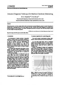
The close relation between the vibration amplitude and αL has been observed in practical machining tests, see Chapter 4. Measuring of the Lissajous angle may provide additional information about the stability of the machining process. However, the vibration amplitude is not necessarily related to the stability of the machining process since i) a stable machining process working close to resonance is still stable ii) a rough machining system is still stable, but with higher dynamical forces causing the higher vibration amplitudes. Furthermore, information about the vibration amplitude may only be obtained up to the saturation level, i.e. the limit when the Lissajous figure shows an enclosed arc. It can however be questioned whether Lissajous figures are suitable for condition monitoring of machining processes due the the following factors:
• limited to inactive feed axes only, • fails to produce a clear arc if the energy in the response from the encoder is low, • ambiguous situation when saturation of αL occurs, which restricts the method to smaller vibration amplitudes, • unable to discriminate between forced vibration and more severe forms of vibrations 30
Machining processes naturally generate forced vibrations which are generally not severe. Instabilities on the other hand are often caused by self-excited vibrations (chatter), which may lead to severe vibration amplitudes and consequently a machining process failure and poor surface quality and integrity of the machined part if not handled properly. The vibration amplitude may reach a level such that it cannot be detected by measuring of αL due to saturation when αL → 2π. Even though the Lissajous method suffers from the aforementioned drawbacks, the implementation of the method is relatively straighforward since it only takes the encoder signals Ua and Ub as input, which are available in modern CNC machine tools.
3.3.2
Formation of Lissajous figures from samples
The formation of a Lissajous figure from scalar time series requires that a sufficiently large number of samples are collected from the sample sequencies {Ua } and {Ub }. Accumulation of all the data points from {Ua } and {Ub }, especially from long time series is not appropriate since the Lissajous diagram will soon be overcrowded and the Lissajous figure will most likely end up in an enclosed arc, thus giving no useful information at all. Instead, the input samples to form the Lissajous figure can be selected using a running window approach. Furthermore, the selected window length L must be large enough to contain a sufficient number of pairs from the sequencies. For practical machining cases, the spindle reference mark signal Ur can be used to identify each spindle revolutions. It is therefore convenient to have a window length that corresponds to the period of one spindle revolution, e.g. a spindle speed of 280 rpm and sampling rate 20 kHz gives a window length of 4286 samples. Samples from the sequences {Ua } and {Ub } can then be collected between subsequent pulses to form the Lissajous figure. When using the windowing appraoch, a function αL (k), i.e. the included angle in the Lissajous figure as function of the discrete time k, can be obtained, see Figure 3.9. Overlapping windows may also be considered to increase the resolution of αL (k). This technique is used when analysing the time series in Chapter 4. 31
αL (k) [rad]
2π
π
0
10
20
30
40
50
60
70
80
90
100
k Figure 3.9 – Lissajous included angle as function of discrete time k measured using a running window over subsequent spindle revolutions.
It has also been observed in practical machining tests that the arc will not stay in a fixed location in the Lissajous diagram during the machining process for subsequent spindle revolutions. Instead, the arc tend to circulate about the periphery of the circle, which complicates the calculation of the included angle from a set of points {Ua (n), Ub (n)} where n = 1, 2, . . . , L. A numerical method to carry out the computation has been developed and implemented by the author and included in the Appendix in this thesis. As will be seen in Chapter 4, the resulting Lissajous angle, when using the windowing technique, also shows a strong correlation with standard linear first-order statistical moments, such as the mean and variance, of the scalar time series. The Lissajous angle may therefore be used to measure the stationarity in the data.
3.4
Hilbert transform
The Hilbert transform (HT) is a linear operator that can be used to extract the instantaneous frequency of a signal. For an arbitrary signal x(t), its HT y(t) is defined as5 y(t) = 5
32
1 � ∞ x(τ ) P dτ π −∞ t − τ
The P preceeding the integral in Eq. 3.10 denotes the Cauchy principal value
(3.10)
from which it can be noticed that the HT is basically the convolution of the 1 , which makes it capable of identifying local properties of signal x(t) with πt x(t). The resulting analytical signal has a real and imaginary part, and given as z(t) = x(t) + jy(t) = a(t)ejϕ(t)
(3.11)
The instantaneous properties of x(t) are defined as �
a(t) =
x2 (t) + y 2(t)
(3.12)
and � −1
ϕ(t) = tan
y(t) x(t)
�
(3.13)
where a(t) is the instantaneous amplitude of the signal x(t) and ϕ(t) is the instantaneous phase of x(t). The instantaneous frequency ω(t) is defined as the time derivative of the instantaneous phase ϕ(t) as follows ω(t) =
d ϕ(t) dt
(3.14)
There are some restrictions regarding which type of signals that can be analysed with the HT. Signals in general are classified as mono-component or multi-component. The HT can only be applied to the first class of signals, i.e. mono-component signals, also known as ”Hilbert-friendy”. An example of this class of signals is the well known chirp-signal with a time-varying frequency as shown in Figure 3.10, but also ordinary sinusoidal signals [18]. Chirp-like signals generally arise from the acceleration and deceleration of moving or rotating masses.
y(t)
1 0 −1 0
2
4
6
8
10
t Figure 3.10 – Chirp-signal with linearly increasing frequency, y(t) = sin(2πf (t) · t), f (t) = kt, k = 0.2. 33
The response from position encoders for active machine axes are frequency modulated sinusoids. Since signals with a frequency that varies nonlinearly with time are mono-component, these signals may be analysed using the HT as they represent a general form of a chirp-signal. The response from inactive feed axes on the other hand are super-positioned sinusoids, i.e. multi-component, and cannot be analysed using the HT.
U(t)
ϕ(t)
The process to obtain the modulation signal from a frequency-modulated signal is illustraded in Figure 3.11. The phase of the mono-component signal in 3.11 (a) is shown in 3.11 (b). The unwrapped phase ϕu (t) in 3.11 (c) corresponds to the position signal. The final modulation signal in 3.11 (d) is obtained by removing the linear component from the position signal.
t
t (b)
Δϕ(t)
ϕu (t)
(a)
t
t (c)
(d)
Figure 3.11 – Demodulation process using the HT. (a) Original signal. (b) Phase of the analytical signal. (c) Unwrapped phase/position signal. (d) Modulation signal. Since the resulting phase in Eq. 3.13 will be in the range [−π, π], it is necessary to first ”unwrap” it to obtain the phase in the form ϕu (t) = ω0 t + Δϕ(t) = 2πf0 t + Δϕ(t)
(3.15)
where ϕu (t) denotes the unwrapped phase in [rad], ω0 is the steady-state angular frequency in [rad/s], Δϕ(t) is the modulation signal in [rad] . 34
The HT is very useful when dealing with frequency modulated encoder signals from various machining processes. During machining, the signals from active machine axes will undergo frequency modulation. The modulation can be regarded as the sum of several effects in the machining process, such as vibrations, variations in the workpiece material and tool wear. The signals may also contain undesirable components, resulting from the acceleration/deceleration of moving masses, friction force in the guideway, direction change, etc.
3.4.1
Separation of the modulation signal from the unwrapped phase
When analysing the response from position encoders for an active machine axis, the HT is can only be used to calculate the position signal (or unwrapped phase), see Figure 3.11 (c). Since the signature of the machining process is initially ”hidden” in the position signal as the modulation signal, the main problem is to separate the modulation signal from the position signal. This will be refered to as the demodulation process. Once the modulation signal has been extracted, small variations, such as torsional vibrations and variations in the feed directions, can be analysed. The modulation signal is extracted by removing the linear term ω0 t in Eq. 3.15 through linear detrending, filtering or differentiation of the position signal. Filtering of the position signal requires that the carrier frequency is known, which can be determined by using Eq. 3.1 or Eq. 3.2. However, detrending and filtering may fail or produce poor results in occasions when the spindle speed or feed rate is non-constant. Differentiation of the position signal gives the instantaneous velocity but is very noise-sensitive and a more advanced analysis may be required in order to extract the useful information. Other methods to separate the modulation signal Δϕ(t) from the position signal may also exist. If the demodulation process performs as expected, regardless which method is used, the carrier component will be removed and the sideband frequencies will now appear in the lower frequency range. The modulation signal, which contains the process-related variations, may then be analysed within an appropriate domain. 35
3.4.2
Scaling of the unwrapped phase
As indicated by Eq. 3.1, there are 256 periods of the near-sinusoidal signals during one spindle revolution. The position signal, or unwrapped phase defined in Eq. 3.15, may be divided by this number to obtain correct scaling of the position signal. The same reasoning applies for the output signals from the linear encoders. Eq. 3.3 gives that the near-sinusoidal signals contain 50 cycles per millimeter movement. To convert the modulation signal in length units, the angular values must be divided by the number of periods per length unit to obtain correct scaling. However, correct scaling is not critical for the analysis and can therefore be left out.
3.5
Hilbert-Huang transform
The Hilbert-Huang transform (HHT), was originally developed by Huang et al. [19]. The method is based on the HT (see Section 3.4) and results in a timefrequency representation of the data. It was originally developed to handle problems due to insufficient number of samples, nonstationary data and nonlinear data. The key strength of the method is the use of the instantaneous frequency defined in the HT in Eq. 3.10. As mentioned in Section 3.4, the drawback with the HT is the fact that it is limited to mono-component signals only. The HHT solves this issue by first decomposing the signal into so called Intristic Mode Functions (IMFs) through a process called the Empirical Mode Decomposition (EMD), also known as the sifting process. The EMD is a pre-processing step which decomposes the original signal into a series of separate oscillatory modes. In an ideal decomposition, all modes of oscillations, i.e. the IMFs, will be mono-component, to allow the use of the Hilbert Transform to determine all the instantaneous frequencies in the signal. A drawback with the HHT is that it suffers from not beeing able to tell in advance the number of resulting IMFs generated in the EMD process. Furthermore, some of the genaretd IMFs may not actually correspond to the physical phenomena [20]. The results must therefore be carefully interpreted. Some improvements to the original HHT have lately been reported, e.g. [18, 21], addressing the issue with the stop criterion in the sifting process. 36
3.6
Nonlinear time series analysis
The HT and HHT methods presented in previous sections have shown to be useful in the preprocessing step of the measured signals and used mainly to transform the original signals into some meaningful data, such as the modulation part of the signals. TF analysis can provide some insight into the process dynamics, but must be supplemented with additional tools to get a more complete picture of the dynamics of the machining process. The set of tools used to analyse the measured signals must be expanded since the output signals from machining processes show nonlinear periodicites and linear tools are not well suited for the task. Even the simplest machining process, such as orthogonal cutting, may show chaotic behaviour where the level of chaos is dependent on the workpiece material [22]. A dynamic system, given as a differential equation, such as x˙ = (x, t) is generally analysed using its phase space description which gives time evolutions of its state trajectory. The dimension of the phase space is related to the number of independent state variables. For systems with dimensions higher than three it is difficult to look at their phase space. The study of the flow in phase space can reveal interesting details about the system, such as the existence of limit cycles and stable, chaotic and strange attractors, but is also useful for the prediction of its future states. For practical systems, mathematical models of the system are commonly unavailable, making an analytical investigation very difficult. However, the nonlinear theory allows the reconstruction of the system from measurements of one or more representative and independent state variables. The most important reconstruction technique is the embedding of a single measured variable into a delay coordinate vector xn = [xn , xn−τ , . . . , xn−(m−2)τ , . . . , xn−(m−1)τ ]
(3.16)
where m denotes the embedding dimension and τ is the reconstruction delay. The (m, τ ) forms the embedding parameters. The delay coordinate vector represents a time separation of the measured time series x. The most important property of this method is the preservation of the most important aspects of the system dynamics, indicated by the fact that the reconstructed phase space has similar geometric properties as the true phase space. The analysis can then be performed using the pseudo phase space. In the preceeding steps, the embedding parameters must be determined in the 37
following order:
1. determine the optimal embedding delay 2. determine the minimum embedding dimension
3.6.1
Mutual information
The mutual information function presented by Fraser and Swinney [23], is unlike the autocorrelation function, a measure of the dependence between samples as it also takes into account nonlinear correlations. The computation of the mutual information function for a scalar time series is based on partitioning of the data into intervals (or bins), and defined as I(τ ) = −
� i,j
pi,j (τ ) ln
pi,j (τ ) pi pj
(3.17)
where pi is the probability of finding a sample in the ith interval, and pij (τ ) is the joint probability of finding a sample in the ith interval which a time τ later is found in the jth interval. The optimal delay value is then be found by considering the first minimum of the mutual information function.
3.6.2
Embedding dimension
A method to determine the minimum required embedding dimension is the method of false nearest neighbours (FNN) originally proposed by Kennel et al. [24]. The minimum dimension must be large enough to fully resolve the system’s phase space. Using a smaller value than the minimum required, points on the phase space trajectory will be projected into the vicinity of other points with which they are not really neighbours, but false neighbours. The FNN method starts with a low dimension and then increases it step by step until a sufficiently low number of false neighbours exist. If x(j) is the nearest point to x(i) for an embedding dimension m, the distance between these points is given by 2 rm (i, j) = (x(i) − x(j))2 + . . . + (x(i + (m − 1)τ ) − x(j + (m − 1)τ ))2 (3.18)
38
Increasing the embedding dimension from m to m + 1 the distance will take the form 2 (i, j) = (x(i) − x(j))2 + (x(i + mτ ) − x(j + mτ ))2 rm+1
(3.19)
Then if |x(i + mτ ) − x(j + mτ )| > RT (3.20) rm the nearest neighbor at time i is considered as false. The threshold value RT is set to 10 ≤ RT ≤ 50. The embedding dimension then converges to a characteristic value as the percentage of FNNs drops to zero.
3.6.3
Chaotic invariants
Various methods for the quantification of dynamic systems are presented. The correlation dimension is a measure of the complexity of the geometry and shape of the attractor, while Lyapunov characteristic exponents can be used to distinguish between chaotic or nonchaotic behaviour. A method to estimate the correlation dimension was originally presented by Grassberger and Procaccia [25]. A hyper sphere with a small radius of ε is centered on the attractor. Let Nx (ε) denote the number of points on the attractor that are inside the sphere. When ε is increased, the number of points inside the hyper sphere will increase exponentially. To account for the variation of the pointwise dimension over the attractor, the average of the number of points is often computed, also known as the correlation sum, defined as N � N � 2 C(ε) = Θ(ε − �xi − xj �) (3.21) N(N − 1) i=1 j=i+1 where Θ is the heaviside step function. The correlation sum is a measure of the number of pairs (xi − xj ) whose distance is less than the radius ε. For an infinite number of points, i.e. when N → ∞ and for small value of ε, the correlation sum is expected to scale according to the power law C(ε) ∝ εd
(3.22)
The correlation dimension is then defined as the local slopes of the correlation sum, given as log C(ε, N) (3.23) d(N, ε) = log ε 39
d = lim lim d(N, ε)
(3.24)
ε→0 N →∞
In time series analysis, it is desirable to avoid temporal correlations, such as those occurring when samples are close in time and correlation due to the geometry of the attractor. A modified definiton of the correlation sum formula is used to exclude such temporal correlations. C(ε) =
N N � � 2 Θ(ε − �xi − xj �) (3.25) (N − nmin )(N − (nmin − 1)) i=1 j=i+nmin
Here, the value of nmin can be chosen freely as long as τ > nmin � N
(3.26)
where τ is the lag that gives the first zero-crossing in the autocorrelation function, and N is the number of data items. To find an appropriate value of nmin , the time-space separation plot can be used [26]. While correlation dimension is a measure of the complexity of the dynamic system, Lyapunov exponents measure the level of chaos in the system. An important property of chaotic systems is their sensitivity to small changes in their initial conditions which have the effect that the state trajectory may diverge after some time. The Lyapunov exponents measure the divergence of nearby trajectories in the phase space. To measure the divergence, two points xn1 and xn2 in phase space, are considered. Their distance is �xn1 − xn2 � = δ0 � 1. Following the trajectory a small time step Δn into the future from these two points, their distance is �xn1+Δn − xn2+Δn � = δΔn . The Lyapunov exponent is then defined as [26]. δΔn ∝ δ0 eλΔn ,
δΔn � 1,
Δn � 1
(3.27)
The number of Lyapunov exponents that can be expected for a dynamic system is determined by the dimension of the phase space. The Lyapunov spectra is therefore given as λ1 , λ2 , . . . , λn ,
λ1 ≥ λ2 ≥ · · · ≥ λn
(3.28)
It is however not always necessary to calculate the entire spectra of exponents. According to Rosenstein et al. [27] it is sufficient for most applications to calculate the largest exponent λ1 to characterise the system. A positive value of the largest exponent is an indicator of chaotic behavior. A large negative value reflects the existence of a stable fixed point, which is characteristic for dissipative systems. 40
3.6.4
Poincaré sections
Poincaré sections are used extensively to transform complicated behaviour in the phase space to discrete maps in a lower dimensional space, where the system dynamics can be analysed from a point-to-point basis, see Figure 3.12. When the phase space is overcrowded, a Poincaré section can be used to reveal the underlying structure of the attractor. The Poincaré section is obtained by following the trajectory and collecting successive intersection points with the surface of section S. The state trajectory may cross the plane from two directions - either from the negative or positive side of S. It is however sufficient to record the crossings from one direction only, which produces the single-sided Poincaré section.
1 0.5 q3
0 −0.5 −1 1 0.5
1 0.5
0 −0.5 q2
−1 −1
0 −0.5 q1
Figure 3.12 – Making of Poincaré section with an arbitrary planar surface of section. The mapping function P from one point on the surface S to the next is defined as P :S→S
(3.29) 41
The discrete Poincaré map P is the mapping function between successive returns on S and is defined as rn+1 = P (rn )
(3.30)
where P is the mapping function and rn is the nth return on S. The Poincaré sectioning can be performed in various ways. For periodic non-autonomous systems the system can be sampled using some natural periodicity of the system, which would not require any embedding of any state variables. For autonomous systems, such as those represented by embeddings, the embedded phase space is instead cut by a surface of section which is often fixed at one of the delay vectors, thus reducing the dimension by 1. Since time information will only be implicitly available in the return map, it can be supplemented with the time of first return function τ (xn ), sometimes referred to as the ceiling function, which gives the time between successive returns. For a trajectory starting at point xn , the total time is given by the cumulative time, defined as tn+1 = t0 + τ (xn ),
t0 = 0,
xn ∈ S
(3.31)
Other quantities, such as distance between successive returns, can be defined in a similar manner. The Poincaré section is constructed using one of the following approaches [26]: • delay embedding of time series and collecting of intersection with the surface of section, • stroboscopic map, collecting of one sample per driving period, • collecting of the minima or maxima of the time series and plotting the values using a delay value of 1 For the time series from the slot-milling process, sampled at 20 kHz with a near constant driving period of 0.2143 seconds (60/280), there are approximately 4286 possibilities to convert the data into map data by a stroboscopic view. Visualisation of the Poincaré data becomes an issue for higher dimensional embeddings, i.e. when the embedding dimension m > 4. In such cases, projection of the data to lower dimensional subspaces is necessary to allow visual inspection of the phase space. Some important methods are the principal component analysis (PCA), singular value decomposition (SVD), and Wavelets. 42
These methods allow the data to be represented in lower dimensional space, but may also involve some loss of information.
3.7
Selection of signal analysis methods
The signal analysis method presented in this chapter may be used to extract additional information about the machining process condition from the response of the position encoders for multi-axis CNC machine tools. The type of response to expect from the encoders is mainly dependent on whether the encoder is sitting on an active or inactive machine axis. A position encoder mounted on an inactive feed axis senses the forced vibration in the direction of the axis. Thus, the energy content in the response is then dependent on the size of the force component acting in the direction of the axis and therefore also dependent on the rigidity of the axis, which determines the ability of the axis to withstand the vibration. Figure 3.13 gives a schematic overview of the methods that may be applied when analysing the response from an inactive feed axis.
Figure 3.13 – Schematic overview of signal analysis methods applicable to the response from encoders for an inactive feed axis.
Another factor that influence the choice of analysis method is that the encoder output signals have a limited maximum amplitude. If the vibration amplitude exceeds a critical level, a saturation of the signals will most likely occur. This is a source of uncertainty since the behaviour of the response due to saturation is not yet well understood. 43
The Lissajous figure may provide a rough estimate of the vibration amplitude for inactive feed axes. The formation of the arc requires accumulation of sufficient number of samples, why it is unable to estimate the instantaneous vibration amplitude. The method also suffers from a saturation effect for larger vibration amplitude. It also requires a clear response from the encoder which is not obtained the case in the more rigid feed axis directions. Spectral analysis using the FT and HHT, may be applied to any of the signals and is useful to detect the presence of periodicities in the signals. For an active machine axis, the usefulness of spectral analysis is rather limited in the sense that the signals contain a dominating frequency (a carrier), which is directly related to the operational feed rate or spindle speed. The Lissajous method presented in Section 3.3 is not applicable to the response from an active machine axis since the output produces an enclosed arc in the Lissajous figure. For an active machine axis, the focused is instead on the analysis of the phase modulation of the carrier component. The HT combined with unwrapping of the instantaneous phase provides an efficient means of evaluating the position signal. The main issue is however to separate the modulation signal from the position signal. Analysis in the frequency domain and phase space domain may then be carried out using the modulation signal as input. Figure 3.13 gives a schematic overview of the methods that may be applied when analysing the response from an active machine axis, such as an active feed axis or active spindle.
Figure 3.14 – Schematic overview of signal analysis methods applicable to the response from encoders for an active machine axis. The first criteion to extract relevant and reliable information about the machining process is that the signal being analysed actually contains the processcharacteristic frequencies. The response for an active machine axis do not 44
initially contain the operational frequencies due to the existence of a carrier component, which in general may also be time varying. Additional preprocessing of the incoming signals is needed in this case to extract the useful part of the signal, which in this case is the modulation signal. The HT is used to obtain the position signal for an active feed axis or active spindle. The disturbances that occurs in the machining process can be found in the modulation signal which must be separated in order to be analysed. The operational frequencies can then be found by performing the FFT or HHT of the modulation signal. No general method for the separation of the modulation signal has been presented. The simplest method is using linear detrending of the position signal but may lead to spurious results if applied to the whole time series. Best results are obtained when performing the detrending operation for stationary parts of the measured time series. Sicne the modulation signal is highly nonlinear, the analysis may be supplemented by additional tools, such as nonlinear time series analysis in the phase space obtained by reconstruction from the modulation signal. The Poincaré sectioning technique may be used to produce a point-to-point representation of the dynamics, which also requires accumulation of a sufficiently large number of returns on the surface of section. Depending on the final objective with the condition monitoring, i.e. whether the objective is to characterise the machining process through ”fingerprinting” or detection of sudden failures, one of the following approaches may be used. • monitoring from start to end of the machining process, • monitoring per cutter revolution, • monitoring using short time windows Monitoring from the start to end of a machining operation allows to produce a fingerprint of the machining operation which may later be compared with an ideal machining situation in order to reveal any deviations. Disturbances will most likely be visible in the fingerprint. Monitoring per cutter revolution produces a ”stroboscopic view” of the machining process based on once-perrevolution sampling. In order to detect events that occur within a short time interval, a short time window must be used.
45
Ub
t
t
Ub
0.5 0 −0.5
Ub
0.5 0 −0.5
Ub
0.5 0 −0.5
Ub
0.5 0 −0.5
Ub
0.5 0 −0.5
Ub
0.5 0 −0.5
Ub
0.5 0 −0.5 0.5 Ub
50 rpm 100 rpm 150 rpm 200 rpm 250 rpm 300 rpm 350 rpm 400 rpm
Ua
0 −0.5
Ua
Figure 3.15 – Output signals Ua and Ub from the y-axis encoder during unbalanced rotation at 50, 100, . . . , 400 rpm with the corresponding Lissajous figure shown in the third column. 46
Chapter 4 Exeperimental work In this chapter, the experimental work conducted as a part of this thesis, is presented. Much of the deltails regarding the experiments are left out but can be found in the appended papers. Results from unpublished experimental work and later findings which have not been included in the individual papers, can be found in the following subsections.
4.1
4.1.1
Linear encoder response to rotating unbalance Description
The focus in this experiment is primarly to study the response from linear position encoders during periodic excitation. This is important since practical machining operations may invlove simultaneous use of active and inactive motion axes. From Section 3.1 we know that the response from the encoder is different from active and inactive machine axes. To avoid the disturbances or complexities from any machining process, this experiment is designed to allow the study of the response in the non-machining case with no active feed axes or active spindle. During practical machining operations, especially intermittent machining operations, periodic excitations are created naturally from the interaction between the tool and the workpiece. In this experiment 47
however, no machining is taking place and the periodic excitation is therefore created by rotation of the turn table at various speeds and various amount of unbalance, see Figure 4.1. Furthermore, the multitask machine tool used in this experiment is equipped with two turn tables, which allows us to compare the response between these two structural components.
Figure 4.1 – Turn table of the 5-axis multitask machine tool.
The centrifugal force Fc , resulting from inertial effects due to rotation, is a function of the unbalance me and the angular velocity ω, and given as [28] Fc = mu eω 2
(4.1)
where mu denotes the unbalance mass and e is the eccentricity of the unbalance mass. This experiment allows us to play with three different parameters. To get a significant increase of the centrifugal force, the rotational speed was increased in steps of 50 rpm starting at 50 rpm up to the maximum speed of 400 rpm . The output signals Ua and Ub from the linear encoders for the x and y axes were sampled at 1024 Hz. To reduce the number of experiments, all rotational speeds were included in each measurement. In the first experiment, the turn table was rotated according to the aforementioned scheme with no unbalance mass. In the following experiments, an unbalance mass mu (fixed mass) was placed at three different radial distances from the center of rotation as illustrated in Figure 4.2. The excitations were repeated three times per unbalance case and performed on both turn tables. 48
ω
mu
ω
(a)
(b)
e
mu e
mu
ω
ω
(c)
(d)
Figure 4.2 – Unbalance cases.
4.1.2
Signal analysis
The output signals Ua and Ub are measured from the linear encoders for both feed axes x and y. Since these axes are inactive, we know from Section 3.1 that the encoder output signals are multi-component. The signals also include components resulting from the acceleration and deceleration of the rotating table. Only the y-axis signal is considered since the response from the x-axis encoder is relatively small due to the rigidity of the structure in this direction. Figure 4.3 shows the power spectrum of the measured signal Ua for the maximum unbalance case in Figure 4.2 (d). The power spectrum represents the energy content in the signal and thus the amount of information contained at a given frequency. The energy in the signal should therefore increase when increasing the rotational speed of the turn table. From the power spectrum it can be noted that the lower frequencies are not represented, such as the 0.83 Hz component corresponding to 50 rpm. One reason for this is that the signal amplitude in time domain for this frequency is relatively low and will therefore not show up as a distinct peak in the power spectrum. The stepwise increase of the rotational speed from one level to the next involves acceleration of the turn table and mass which will contribute to the energy at the higher frequencies. The power spectrum is unable to reveal when in time the higher frequencies exist. A a time-frequency analysis, TFA, of the signal is therefore considered in order to study the frequency variation in the signal over time. For the nonlinear signal in this case the STFT will produce a poor TF-representation due to its poor frequency resolution. A decomposition of the signal into its 49
Figure 4.3 – Power spectrum of the y-axis encoder signal Ua for the unbalance case (d) in Figure 4.2. The dotted vertical lines indicate the excitation frequencies corresponding to the turn table speeds 50, 100, . . . , 400 rpm.
intristic mode functions using the HHT1 described in Section 3.5 is therefore carried out as shown in Figure 4.4.
f [Hz]
40 30 20 10 0 0
10
20
30
40
t [s] Figure 4.4 – Instantaneous frequency for the y-axis position signal Ua for increasing vibration level, calculated with the HHT for unbalance case (d).
Figure 4.4 shows a time-frequency representation on the signal obtained by the TFA. It shows that the higher frequency components (f > 6.67 Hz) originate from some ranges of the rotational speed, but also from the final deceleration of the rotating mass. 1
50
MATLAB code for the HHT can be found at http://software.seg.org/2007/0003/
To analyse if the measured signals carry any information about the vibration level, the included angle in the Lissajous figure can be calculated. However, this must be performed within short duration time windows. Since the output signals from the rotary encoder of the turn table were not acquired in this study, segmentation of the linear encoder signals based on the revolution of the turn tables is not possible. Instead, the measured time series were split into segments of length 300 samples, giving a sufficient number of input samples to the Lissajous figure. Then, by performing the calculation of the Lissajous included angle of each segment (see Section 3.3), will yield an approximation of the time evloution of the included angle from the start to the end of the excitation, see Figure 4.5.
αLissajous
2π
π
0 0
50
100
150
k Figure 4.5 – Calculated included angle of the Lissajous figures. The dotted curve indicates a quadratic increase of the vibration amplitude. The measured included angle in Figure 4.5 increases quadratically with increasing speed, which is in agreement with Eq. 4.1. There is obviously a strong correlation between the Lissajous included angle and the vibration level, at least up to the saturation limit reached when the Lissajous figure shows an enclosed arc. Consequently, the measured time series contains information about the dynamics of the system of rotating unbalance. Next, the scalar time series are analysed using nonlinear analysis presented in Section 3.6. The mutual information and the FNN method are used to estimate the embedding parameters. The first minimum M1 of the mutual information in Figure 4.6 varies for the different unbalance cases (a)-(d) according to: (a) 37, (b) 49, (c) 40, (d) 49. The fraction of false neighbours also show small variations depending on the unbalance case, but tend to drop to zero when m > 3 with 1 − 2% false 51
I(τ )
0.5
0.25 M1
0 0
50
100 τ
150
200
Figure 4.6 – Mutual information for the y-axis signal Ua for the unbalance case (d) with first first minimum at τ = 49.
Fraction of f.n.n.
0.5
0.25
0 1
2
3
4
5
6
7
8
m Figure 4.7 – Determining the embedding dimension using the FNN method.
neighbours when m = 4. In this study, the time series is embedded in a 3dimensional space, accepting 7 − 11% of false neighbours in the embedding space. The Poincaré sectioning is then performed by following the trajectory in the reconstructed phase space and collecting the crossing points with the surface of section plane. The resulting Poincaré sections will be different depending on the actual unbalance situation, as shown in Figure 4.8. 52
(a)
(b)
(c)
(d)
Figure 4.8 – Poincaré sections for unbalanced rotation of turn table I.
4.1.3
Results
The most important results from this experiment are that the vibration from rotating unbalance is sensed by the position encoders, but it also shows that the output signals for an inactive machine axis is multi-component, i.e. they can be represented by superpositioned sine waves, which is shown in the amplitude spectrum of the signals. From the analysis of the rotating unbalance experiment it has been observed that • the encoder response from the less rigid y-axis is stronger than the response from the x-axis, • the amount of unbalance affects the strength of the response, which results in higher SNR values, • the rotational frequencies appear as distinct peaks in the power spectrum, and • the Poincaré sections shows a unique pattern for each unbalance case
53
4.2
4.2.1
Machining of aerospace component industrial trial Description
The work presented here is carried out during a pre-production by Volvo Aero Corporation in order to validate a machining process used to create special features on an aerospace component before real production. A disc-milling operation is considered using a 9-flute milling cutter and spindle speed of 400 revolutions per minute, see Figure 4.9.
Figure 4.9 – Disc milling cutter with 9 flutes. During the testing, the response from the internal position encoders of the machine tool is measured in order to perform analysis of the signals and investigate the usefulness of various analysis methods. The output signals from a linear position encoder and a rotary encoder are considered, see Table 4.1. The active machine axes in this machining process is the feed axis y and the main spindle axis S1. The second feed axis x is an inactive axis. The signals are measured from the start to the end of the machining operation. No signals are measured from the linear encoder for the active feed axis y during operation. The actual sampling rate is set to 8192 Hz. According to Eq. 3.1 the main frequency in the S1-axis signals Ua and Ub is 1707 Hz which is below the Nyqvist frequency 4096 Hz. The tooth-passing frequency is 60 Hz according to Eq. 3.5 which is expected in the response from the linear encoder for the inactive machine axis. A typical response from the x-axis encoder is shown in Figure 4.10. A decrease 54
Table 4.1 – Recorded signals during the disc-milling operation. Machine axis x S1
Signals Ua , Ub Ua , Ub , Ur
of the amplitude can be noted at t ≈ 30 s. This effect is observed in all nine tests and may be due to variation of the actual cutting parameters for the actual machining operation. It is desirable to remove all the non-machining segments from the measured time series so that only the most important aspects are included in the analysis.
Figure 4.10 – Typical response from the x-axis position encoder during the disc-milling operation. The initial end ending parts represent non-machining and the middle part represents machining. The responses from the rotary encoder for the S1-axis is seen in Figure 4.11.
4.2.2
Segmentation of the measured signals
The segmentation of the measured signals is performed by considering the pulses found in the reference mark signal Ur . The pulses are well defined as can be seen in Figure 4.11 and can be numerically detected by calculating the first-order difference of the sequence {Ur }. Spurious pulses may be removed using thresholding and initial knowledge about the minimum time between the pulses. 55
Amplitude (Volts)
Reference mark signal
Time (s)
Figure 4.11 – Typical response from the S1-axis position encoder during the disc-milling operation.
The spindle speed can then be estimated by evaluating the time between two subsequent pulses. Table 4.2 shows the number of recorded spindle revolutions after removing the non-machining segments from the signals, minimum and maximum spindle speed, the average and standard deviation of the spindle speed for all nine machining cases. It can be noted that the spindle speed is kept almost constant at 400 rpm. Notice that the length of the recordings varies between the machining cases due to variations of some process parameters. Some operations are also interrupted leading to shorter recordings. This step is always taken in the offline analysis of the signals to ensure that the segmentation of the signals has performed well. Table 4.2 – Spindle speed statistics calculated from the reference mark signal Ur . Case 1 2 3 4 5 6 7 8 9
nrev nmin [rpm] nmax [rpm] n ¯ [rpm] σn [rpm] 155 399.35 400.65 400.01 0.1199 127 397.74 401.96 400.01 0.2808 106 395.81 401.31 399.96 0.4876 81 399.03 400.65 400.01 0.1666 177 396.77 401.64 399.99 0.3534 179 399.03 400.65 400.01 0.1311 80 397.74 401.31 399.98 0.4182 47 399.03 400.98 400.02 0.2444 83 394.54 400.98 399.92 0.7179
The calculated spindle speeds confirm a stable spindle speed during the machining operation but do generally not give any useful information about the dynamical aspects of the machining process. 56
One way to obtain better insigt into the machining process is to study the machining process per spindle revolution. The measured encoder signals Ua and Ub from the x-axis and the position signal from the main spindle are therefore considered. The signals are cut into shorter segments, where each segment corresponds to a cutter revolution. The length of the segments will vary due to minor variations in the estimated spindle speed as given in Table 4.2.
4.2.3
Vibration amplitude estimation from the Lissajous figure
Figure 4.12 shows the included angle in the Lissajous figure formed by the pairs {Ua , Ub } over subsequent revolutions of the milling cutter. A notable saturation occurs within segments 80 < k < 100 which may be an indication of relatively tough machining within the corresponding time interval.
αL(k) (rad)
2pi
pi
0
20
40
60
80
100
120
140
k Figure 4.12 – Included angle of the Lissajous figure obtained from the pairs {Ua , Ub } calculated over subsequent cutter revolutions. In a similiar way, the sequences {Ua } and {Ub } can be evaluated by calculating the running variance and RMS-value over subsequent cutter revolutions, which is shown in Figure 4.13 and Figure 4.14. The running variance and RMS-value of the sequences Ua and Ub show strong correlation with the included angle of the Lissajous figure. Since the Lissajous included angle is proportional to the vibration amplitude (up to the saturation level 2π radians) as stated in Eq. 3.9 in Section 3.3, it is reasonable to believe that these quantities also carry some information about the vibration amplitude in the machining process as well. 57
0.15
σ2
0.1
0.05
0
20
40
60
80
100
120
140
k Figure 4.13 – Running variance of the x-axis signals Ua and Ub calculated over subsequent cutter revolutions.
0.5
URM S
0.4 0.3 0.2 0.1 0
20
40
60
80
100
120
140
k Figure 4.14 – Running RMS-value of the time series Ua and Ub calculated over subsequent cutter revolutions.
4.2.4
Analysis of the rotary encoder signals
The main spindle holding the milling cutter is responsible for the energy input to the machining process. The spindle is designed to be very stiff in order to provide enough torque to the milling cutter for the removal of material from the workpiece, but also to withstand torsional vibrations generated in the intermittent machining process. Since the spindle is an active machine axis in this case, the output signals Ua and Ub from the rotary encoder will be near-sinusoids with a main frequency that is proportional to the actual spindle speed according to Eq. 3.1. Using a spindle speed of 400 rpm the main frequency in the signals will be 1707 58
Hz. However, due to the intermittent nature of the process, it is likely that additional frequency components related to the machining process will appear in the output signals. To carry out the analysis of the rotary encoder signals, the spindle position φ is first calculated from either the Ua or Ub signals using the Hilbert Transform, HT, see Section 3.4. After unwrapping of the phase and subtracting the offset, the spindle position as function of time φ(t) where φ(0) = 0, is obtained.
φ(t) (radians)
Figure 4.15 shows a typical spindle position signal. The original signal from 1 the HT process has been multiplied by the factor 256 to get correct scaling. To ensure the correctness of the result, one may also compare the maximum value φmax with 2πN where N is the number of segments (or cutter revolutions) selected for the analysis. However, scaling is not necessary in order to carry out the analysis.
800 600 400 200 0
0
5
10
15
20
t Figure 4.15 – Spindle position signal calculated from the Ua signal from the rotary encoder. The spindle position signal shown in Figure 4.15 resembles a linear function, starting at the origin where the slope of the line is proportional to the angular velocity ω, i.e. φ(t) = ωt. Linear regression analysis of the spindle position samples also gives a strong linear correlation coefficient, which is very close to 1, but gives also that there are some unexplained variation, i.e. deviation from the ideal straight line. In fact, these variations appear as small fluctuations on the straight line, originating from phase-modulation of the original spindle positions signals Ua and Ub . Thus, in order to extract the process variations using the rotary encoder signals, the carrier component (or linear part of φ) related to the spindle speed, needs to be removed from the spindle position signal to produce the modulation part of the signal. 59
ϕ(t) (radians)
−3
3
x 10
2 1 0 −1 −2 10.35
10.4
10.45
10.5
10.55
10.6
10.65
10.7
10.75
t Figure 4.16 – Modulation signal extracted from the spindle position signal during three cutter revolutions, obtained by detrending of the original position signal.
Figure 4.16 shows a characteristic modulation signal during three cutter revolutions in the disc-milling process. The modulation signal shows a nearperiodic behaviour between subsequent cutter revolutions, but also nine distinct peaks within a cutter revolution. Hence, in this case a 9-flute milling cutter is used. Thus, the peaks may therefore originate from the intermittent nature of the milling process. As can be noted, the modulation signal also contains a noise component. However, the process of extracting the modulation part from the spindle position signal by removing the linear component, i.e. through a detrending operation, may produce some undesired effects on the final modulation signal, such as linear trends and sudden drops of the amplitude as shown in Figure 4.17. It is unrealistic to think that the effects shown in Figure 4.17 originate from the machining process. This observation leads to the conclusion that linear detrending may not always be suitable in order to extract the modulation part from the position signal.
4.2.5
Phase space reconstruction
The spindle modulation signal in Figure 4.19 evolves nonlinearly with time. One way to analyse the signal is by using nonlinear time series analysis in the reconstructed phase space as desribed in Section 3.6. 60
Δϕ(t) (radians)
0 −2 −4 −6 0
5
10
15
t Figure 4.17 – Artefacts in the modulation signal produced by detrending of the calculated position signal.
−9
x 10
σ2
3 2 1 20
40
60
80
100
120
140
k Figure 4.18 – Running variance of the de-noised S1-axis modulation signal calculated over subsequent cutter revolutions.
The nonlinear analysis begins with an estimation of the optimal embedding parameters, i.e. the reconstruction delay τ and the minimum embedding dimension m. For a stationary part of the signal, the optimal embedding delay value gives a minimum in the mutual information function I(τ ) defined in Eq. 3.17. However, applying the method directly to the modulation signal will lead to poor estimation of τ as shown in Figure 4.20. The MI function shows numerous spurious minima which, if used as a reconstruction delay, would lead to very poor embeddings. The fluctuations in I(τ ) originate from the noise content in the original modulation signal. Thus, the noise must first be suppressed by filtering of the modulation signal. 61
1
ϕ [rad]
0.5 0 −0.5 −1
0
500
1000
1500
2000 sample
2500
3000
3500
Figure 4.19 – Spindle modulation signal during three revolutions indicated by the dotted vertical lines.
I(τ )
2
M1 1
0
0
50
100
150
200
τ Figure 4.20 – Mutual information of the modulation signal during three spindle revolutions (segments 220-222).
The mutual information of the filtered signal gives the first minima at τ = 34 which is considered as the optimal delay when embedding the time series. The use of mutual information to estimate the optimal reconstruction delay for the final embedding requires careful judgement. It is essential to understand that the first minimum will occur at different value of tau depending on which part of the time series is used as input to the calculation. A good initial guess is to set τ to approximately one quarter of the ”driving period”, as in this case the pariod of one tooth-pass (60/400/9/4 ≈ 34). To estimate the embedding dimension, the merged segments 220 − 222 of the filtered modulation signal is used with the previously determined delay value of 34. The embedding dimension is then estimated using the false nearest 62
1
ϕ [rad]
0.5 0 −0.5 −1
0
500
1000
1500
2000 sample
2500
3000
3500
Figure 4.21 – Lowpass filtered spindle modulation signal during three spindle revolutions (segments 220-222). The dotted vertical lines indicate a spindle revolution.
I(τ )
2
1
M1 0
0
50
100
150
200
τ Figure 4.22 – Mutual information of the filtered modulation signal during three spindle revolutions. First minimum is found at τ = 34.
neighbours method. As can be seen in Figure 4.23, the FNN method suggests an embedding in two dimensions, for which the percentage of false nearest neighbours drops to zero. It is obvious that this is a too low value to be used for the embedding of the nonlinear modulation signal. Performing the calculation over subsequent segments of the modulation signal show similiar results. The FNN method has also been found to produce varying results depending on whether an unfiltered or a filtered time series is used as input. The resulting dimension using the FNN method may also depend on the length of the input sequency and may not always produce stable results [29]. 63
Fraction of f.n.n.
1
0.5
0
1
2
3
4
5
6
m Figure 4.23 – Minimum embedding dimension using the FNN method.
It becomes both necessary and interesting to evaluate the embedding dimension using Cao’s method [29] instead. One of the reported strenghs with Cao’s method is that it does not contain any subjective parameters and the resulting embedding dimension is not strongly dependent on the length of the time series and produces more stable results. The OpenTSTOOL [30] implementation of the Cao’s method is used for the calculation. The resulting dimension estimating using Cao’s method is shown in Figure 4.24. As can be noted, the suggested embedding dimension is somewhere between 4 − 5, indicated by a breakpoint in the graph. This is at least twice the value suggested by the FNN method. 1
E1(d)
0.8 0.6 0.4 0.2 0
1
2
3
4 5 Dimension (d)
6
7
8
Figure 4.24 – Minimum embedding dimension using Cao’s method.
Figure 4.25 shows the final reconstructed phase space in the three coordinates q1 , q2 and q3 , corresponding to the time-delayed vectors x(k), x(k − τ ) and x(k − 2τ ) respectively. Here, shown for three spindle revolutions for the sake of clarity. 64
q3
q2
q1
Figure 4.25 – Reconstructed phase space from the spindle modulation signal during three spindle revolutions including approx. 3700 samples. Embedding parameters: m = 3, τ = 34.
4.2.6
Results
Practical machining of an aerospace component using a disc-milling operation has been performed. The hardness of the workpiece material resulted in a very tough machining process creating large cutting forces and amplitudes of the vibrations. During machining, the output signals from the position encoders was measured and analysed using both traditional and more advanced methods. The most important findings from the analysis of the industrial trials can be summarised as follows.
• The measured signals show a clear response for the disc-milling process. • Linear detrending of the spindle position signal may produce poor representation of the modulation signal which is mainly due to noise 65
• Filtering of the spindle modulation signal may be required in order to estimate the optimal reconstruction delay from its mutual information function • Spectrum analysis clearly shows the tooth-passing frequency. The existence of both subharmonics and superharmonics also reveals the nonlinear effects in the machining process • The calculated αL for the x-axis clearly reflects the tough machining operation. • A strong correlation is found between αL and the running variance σ 2 of the spindle modulation signal. The phase space of the machining system can be reconstructed from the modulation signal in order to analyse the dynamical aspects of machining system. Phase space analysis has not been carried out in this experiment.
66
4.3
4.3.1
Slot-milling with various number of cutting inserts Description
The disc-milling tests presented in Section 4.2 clearly indicated that the impatcs due to the intermittent interaction between the cutting tool and the workpiece generate translational vibration of the work table and torsional vibration of the main spindle. The experimental work in this section presents a more systematic study of the response from the position encoders for a simple slot-milling operation. The slot-milling operation, also known as full-immersion milling, is an intermittent cutting process where the milling cutter is held in a rotating spindle. The workpiece, which is clamped on the table, is moved toward the cutter at a constant feed rate, see Figure 4.26.
Figure 4.26 – Slot-milling process. Furthermore, the milling cutter may have one or more teeth. The cutting forces are produced when the cutting tool is in the cutting zone, i.e. Fx (φ), Fy (φ), Fz (φ) > 0 when φst ≤ φ ≤ φex , where φst and φex are the cutter entry and exit angles respectively [31]. For the slot-milling operation φst = 0 and φex = π. The size of the cutting forces will be time-varying and depends on the number of teeth of the cutter that is cutting simultaneously, but also on the chip width and the varying chip thickness. Thus, for a milling cutter with N teeth, the 67
contribution from teeth j to the cutting forces can be formulated as [31] Fx =
N �
Fx,j (φj ),
Fy =
j=1
N �
Fy,j (φj ),
j=1
Fz =
N �
Fz,j (φj )
j=1
where φj denotes the instantaneous angle of immersion for teeth j. Thus, when φst ≤ φj ≤ φex , the tooth j contributes to the cutting forces. When the tooth j is outside the immersion zone, the contribution is zero. The general parameters of the slot-milling process used in this experiment are given in Table 4.3. Table 4.3 – Slot-milling process parameters. Milling tool 5-flute cutter, carbide inserts Workpiece Inconel 718 Depth of cut 2.0 mm Spindle speed 280 rpm Feed 0.08 mm/tooth Feed rate 112 mm/min Feed direction y Cutting length 50 mm Cutting non-dry All machining parameters are kept constant, except for the configuration of the milling cutter which is altered by reducing the number of teeth on the milling cutter. This will result in a notable increase of the cutting forces and vibration amplitudes. Furthermore, all experimental trials are performed with fresh inserts to minimise the effect from tool wear and to make the results comparable between the different machining conditions or cutting tool configurations. Table 4.4 – Milling cutter configurations. Z1 Z2 Z3 Z4 Z5
1 1 1 1 1
0 1 1 1 1
0 0 1 1 1
0 0 0 1 1
0 0 0 0 1
The various configurations of the 5-flute cutter which correspond to the different experimental cases are listed in Table 4.4. The first column is the name of 68
the cutter configuration and will be referred to in the text. The second column denotes the cutter configuration, where all 0’s indicate the absence of an insert and all 1’s indicate the presence of an insert on the cutter with tooth number (1-5) from left to right. From this it can be noted that in configuration Z2 the second tooth takes three times larger chip thickness than in configuration Z5. The main objective is to investigate the response of the position encoders when performing the machining operation using the aforementioned cutter configurations. The output signals from the rotary encoder on the main spindle (S1), linear encoders on the inactive feed axis x and active feed axis y are digitised at 20 kHz. The measured signals are listed in Table 4.5.
Table 4.5 – Recorded signals during the slot-milling process. Machine axis x y S1
Signals Ua , Ub Ua , Ub Ua , Ub , Ur
At constant feed rate, the feed axis position encoder will give a near sinusoidal output signals, with a main frequency that is proportional to the actual feed rate. During machining, the encoder signals for active feed axes will be distorted by phase modulation, which originate from varying disturbances in the machining process. The analysis of the measured signals is then carried out in the frequency domain using traditional Fourier analysis and within the reconstructed phase space of the system using nonlinear analysis methods. The modulation signal is extracted from the position signal of the active feed axis, which is used as input for the nonlinear analysis. A Poincaré section is then obtained by using the natural period of the machining process. A question here is how the difference show up in the Poincaré sections due to the varying machining conditions. The Lissajous angle is applied to the output signals from the inactive feed axis encoder in order to characterise the vibration amplitude for subsequent revolutions of the milling cutter. The noise content in the output signals from the inactive feed axis encoder is also characterised. The SNR is then estimated for subsequent cutter revolutions. 69
4.3.2
Segmentation of the measured signals
As an initial step in the signal analysis, a segmentation of the measured signals is performed by detecting the pulses in the spindle signal Ur , resulting in segment lengths corresponding to a spindle revolution. In the segmentation process, the starting and ending indices for each segment are recorded each time the spindle passes its reference position (zero angle). The spindle speed is also estimated by evaluating the time between two subsequent pulses, which is an effective way to validate the segmentation process. The segmentation is also useful for the exclusion of the initial and ending non-machining segments from the scalar time series. Table 4.6 shows the number of recorded spindle revolutions nrev after removing the non-machining segments from the signals, minimum and maximum spindle speed nmin and nmax , the average and standard deviation of the spindle speed n ¯ and σn for all experimental trials. It can be noted that the spindle speed is kept almost constant at 280 rpm. Notice that the cutter configuration Z5 only includes a single experimental trial. The small variations in nrev originate from the manual step when selecting the segments for analysis.
Table 4.6 – Spindle speed statistics calculated from the signal Ur . Case Z1
Z2
Z3
Z4
Z5
70
Trial 1 2 3 1 2 3 1 2 3 1 2 3 1
nrev nmin [rpm] nmax [rpm] n ¯ [rpm] σn [rpm] 144 279.98 280.05 280.00 0.0312 147 279.92 280.11 280.00 0.0332 147 279.98 280.05 280.00 0.0313 145 279.92 280.11 280.00 0.0331 145 279.98 280.05 280.00 0.0313 146 279.98 280.05 280.00 0.0313 143 279.98 280.05 280.00 0.0314 144 279.92 280.05 280.00 0.0323 144 279.92 280.05 280.00 0.0323 143 279.92 280.05 280.00 0.0322 143 279.92 280.05 280.00 0.0322 144 279.92 280.05 280.00 0.0323 143 279.98 280.05 280.00 0.0313
4.3.3
Noise characterisation and SNR estimation
Figure 4.27 shows a typical noise signal v(t) and its probability density function (PDF) p(v) measured in the output signal Ua from the position encoder of the inactive feed axis x during this experiment. Noise signal
Noise histogram 0.02 Amplitude
0.02 v(t)
0.01 0 −0.01 −0.02
0.01 0 −0.01 −0.02
Time
0
Autocorrelation of noise 0.5 0 −0.5 −1000 −500
0.2 0.3 p(v) Power spectrum
0.4
50 100 150 Frequency [Hz]
200
0.06 Power
Rvv(τ)
1
0.1
0 τ
500
1000
0.04 0.02 0
0
Figure 4.27 – Typical time history, normalised probability density function p(v), autocorrelation Rvv (τ ) and power spectrum of the noise signal v(t).
• The probability density function p(v) of the noise signal v(t) indicates a nonuniform (Gaussian-like) noise distribution. • The autocorrelation Rvv (τ ) of the noise signal v(t), which is the crosscorrelation of the noise with itself, clearly indicates the presence of a periodic signal buried under the noise. • The power spectrum of the noise signal v(t) obtained by using the FFT reveals that the signal is disturbed by the mains frequency (or utility frequency) 50 Hz. Its contribution to the signal is however considered as relatively small. Figure 4.28 shows a typical time evolution of the SNR value of the x-axis signals Ua and Ub over subsequent revolutions of the milling cutter during 71
the slot-milling operation. The procedure to estimate the SNR value from measured signals is described in Section 3.1.2.
45
SNRdB
40 35 30 25 20
20
40
60
80
100
120
140
k
Figure 4.28 – Estimated SNR value of the signals Ua and Ub from the inactive feed axis encoder over subsequent spindle revolutions.
The SNR values of the two channels Ua and Ub are strongly correlated and show some variation during the machining process. SNR values up to 40 dB have been observed. The lower SNR values found at the initial and final stage of the machining operation are a direct consequence of a weaker response from the encoder for an inactive machine axis.
4.3.4
Measuring of the Lissajous angle from the inactive feed axis signals
The response from the inactive feed axis due to the various cutting conditions is characterised by measuring of the Lissajous angle from the encoder output signals Ua and Ub . Figure 4.36 shows the typical time history of Ua and Ub during three spindle revolutions and the time evolution of the corresponing Lissajous angle αL (k) from the start to the end of the slot-milling process for all five cutter configurations Z1-Z5. A general trend is that the amplitude of αL (k) decreases with increasing number of teeth on the cutter due to improved stability in the machining process. One exception from the general trend can be noted for the case Z1, which should generate the largest impacts, but is obviously not indicated by αL (k). 72
4.3.5
Spectral analysis
The various cutter configurations give rise to different process dynamics due to the nonuniform pitch angle of the cutter in the configurations Z2-Z4, causing uneven loads on the cutting inserts. The cutting insert that immediately follows the gap of missing inserts, will remove more material from the workpiece, resulting in a higher impact on that particular insert. Three of the measured signals has been considered for the analysis: the signal Ua or Ub from the inactive feed axis x, the modulation signal from the active feed axis y, and the the modulation signal from the main spindle S1, as listed in Table 4.7. Table 4.7 – Naming of signals. s1 s2 s3
x-axis signal Ua y-axis modulation signal in Ua S1-axis modulation signal in Ua
Figure 4.29 shows the amplitude spectra of the signals listed in Table 4.7. A dominant peak at 4.67 Hz which corresponds to the tooth-passing frequency (also the cutter frequency) can be noted for cutter configuration Z1. The signals also contain some higher frequency components with decreasing amplitude. Obviously, the frequency distribution is similiar in all these signals, but with varying amount of energy at the specific frequencies. The cutter configuration Z5, which corresponds to the normal machining case, gives a dominant peak at the tooth-passing frequency 23.3 Hz, see Figure 4.30. The amplitude spectra show similiar frequency distribution for the various cutter configurations. The magnitudes at the distict frequencies of the s2 signal are larger than the magnitudes of the corresponding frequencies in the s1 signal, which reflects the lower rigidity of the y-axis for the machine tool used. The spectrum of the s3 signal also indicates a higher damping of the S1-axis. The impacts created in the intermittent milling process represent strong impulses representing a wide range of excitation frequencies. It is therefore possible that some of these frequencies coincide with the natural frequency of 73
Power spectrum 5000 Power
0.5 0
2500
−0.5
0
0.05
30 Power
s1 [Volts]
0
20 10
−0.05
0
0.005
0.5 Power
s2 [mm] s3 [rad]
Time history
0 −0.005 14.8
15
15.2 15.4 15.6 15.8 Time [s]
0.25 0
0
5 10 15 20 25 30 35 40 Frequency [Hz]
Figure 4.29 – Time history of the signals s1 , s2 and s3 during four spindle revolutions and their power spectrum for the cutter configuration Z1. Modulation signals are scaled.
some of the components in the machining system. Figure 4.31 shows a close view at the amplitude spectrum of the signal s3 . The dominant peak found at 1195 Hz may probably be related to the natural frequency of the spindle or the tool holder system. However, this has not yet been verified by any means. This frequency is observed for all cutter configurations Z1-Z5, but the amplitude of the sideband frequencies tends to decrease with increasing number of teeth on the cutter. No such high-frequency content have been observed in the response from the feed axis encoders. 74
Power spectrum 5000 Power
0.5 0
2500
−0.5
0
0.05
30 Power
s1 [Volts] s2 [mm]
0
20 10
−0.05
0
0.005
0.5 Power
s3 [rad]
Time history
0 −0.005 14.6 14.8
15 15.2 15.4 15.6 Time [s]
0.25 0
0
5 10 15 20 25 30 35 40 Frequency [Hz]
Figure 4.30 – Time history of the signals s1 , s2 and s3 during four spindle revolutions and their power spectrum for the cutter configuration Z5. Modulation signals are scaled.
4.3.6
Nonlinear analysis of the active feed axis modulation signal
To analyse the dynamical behaviour of the slot-milling process, nonlinear analysis is used. In the current machining setup, the s2 signal shows a clearer response to process variations and is therefore used as input for the analysis. From the time signals it can be seen that the s2 signal also correlates relatively well with the measured Lissajous angle of the x1 signal which itself is related to the vibration amplitude. The time behaviour of s2 also resembles the time evolution of a vibration signal as shown in Figure 4.32. Notice that the signal is unscaled and the amplitude is presented in radians which originates from the HT demodulation process. The optimum reconstruction delay used in the embedding of s2 is obtained by considering the first minimum M1 in the mutual information of s2 . 75
|S3 (f )|
0.01
0.005
0 1180
1185
1190
1195
1200
1205
1210
f (Hz) Figure 4.31 – Amplitude spectrum of the spindle modulation signal s3 . The distinct peak at 1195 Hz may correspond to the natural frequency of the spindle or tool holder system.
s1 [rad]
3
0
−3
5
10
15
20
25
t [s] Figure 4.32 – Time history of the y-axis modulation signal for the machining case Z1. The leading and ending transients are excluded.
The optimum reconstruction delay values for the different configurations of the milling cutter are tabulatad in Table 4.8. The experiment was repeated three times for all the cutter configuration except for the cutter configuration Z5. It can be noted that the value of τ varies slightly depending on the cutter configuration. Small variations also exists between the replicates. The embedding dimension is then determined using the FNN method. The percentage of false neighbours drops to zero when m = 5 which is the suggested minimum embedding dimension. Figure 4.34 shows three different views of the phase portrait. Due to problems in visualising more than three dimensions, a 3-dimensional embedding is chosen. The final Poincaré section is then obtained by cutting the phase space with a plane located at the average of the data. Figure 4.35 shows a Poincaré section of the y-axis modulation for 76
0.5
I(τ )
0.4 0.3 0.2
M1
0.1 0
0
100
200
300
400
500
τ Figure 4.33 – Mutual information of the y-axis modulation signal for the machining case Z1. First minimum occurs when τ = 212
Table 4.8 – Optimal reconstruction delays. Cutter config. Z1 Z2 Z3 Z4 Z5
τ1 212 234 222 220 196
τ2 207 235 227 216 -
τ3 202 226 234 217 -
the machining case Z1. The section indicate the presence of a stable point at the origin and shows also curve-like structures which indicate quasi-periodic motion along the y-axis.
0
−2
−1
0
x(k − τ )
1
2
x(k − τ )
2
x(k − 2τ )
x(k − 2τ )
2
0
−2
−1
x(k)
0
1
0
−2
−1
x(k)
0
1
Figure 4.34 – Phase portrait of the y-axis modulation for the case Z1.
77
3
0
−3 −3
0
3
Figure 4.35 – Poincaré section of the y-axis modulation for the case Z1.
4.3.7
Phase plane analysis
An alternative appraoch to study the dynamics of the milling process is to obtain the phase plane (or phase portrait) in the form (x, x) ˙ where x is a state variable and x˙ is the time derivative. The Poincaré section may then be constructed by using the natural period of the system by sampling the state trajectory once per cutter revolution, giving a stroboscopic view of the process dynamics. When using a spindle speed of 280 rpm and a sampling rate of 20 kHz, there will be 4286 possibilities to create the Poincaré section. A natural choice in this case is to sample the state trajectory every time the cutter passes the reference position (zero angle). The feed axis modulation signal is the state vector x. The phase portrait is then constructed by numerical differentiation of x. Since differentiation itself is very sensitive to noise, the modulation signal may first be prefiltered to minimise the effects due to noise. A 5th-order Butterworth lowpass-filter with cutoff frequency at 200 Hz may be used to suppress the high-frequency content in the signal without loss of the major aspects of the dynamics. Figure 4.37 shows the resulting phase plane and Poincaré section for each configuration of the milling cutter. Notice that the variables are converted in physical units by scaling of the modulation signal. A notable difference between the Poincaré sections can be observed for the different cutter configurations.
78
4.3.8
Results
In this experiment a single-axis slot-milling operation was considered in order to analyse the response from both linear and angular position encoders for various machining conditions using a 5-axis multitask machine tool. The strength of the impacts between the cutting edges and the workpiece was altered by using various number of teeth on a 5-flute milling cutter. The measured responses have been analysed in the frequency domain and also in the reconstructed 3-dimensional phase space of the machining system. The results from this experiment can be summarised as follows. • The clearest response is obtained from the feed axis encoder for the least rigid machine axis direction, which in this case is the y-axis • Active feed axis signals and spindle signals are phase-modulated and contain information about the process characteristics • Spectrum analysis using FFT indicate that the measured signals from both active and inactive machine axes contain operational frequencies, such as the cutter frequency and tooth-passing frequency, and their subharmonics • The amplitude spectrum of the spindle modulation signal shows that most subharmonics, except the tooth-passing frequency, are highly damped • The energy at the operational frequencies depends on the cutter configuration • The Lissajous angle of the inactive feed axis signals for subsequent cutter revolutions decreases with increasing number of teeth on the cutter • The milling process dynamics may be analysed using the reconstructed phase space of the machining system. A clear difference between the various cutter configurations is shown when creating Poincaré sections using the natural period of the machining system, which is the period of the cutter. The sensitivity to detect phenomena, such as as tool wear, tool breakage, severe vibration has not been the focus in this experiment. This experiment may however be refined to study the responses due to such phenomena. 79
0 −0.5
Lissajous angle αL(k) [rad]
Time history Ub [V]
Ua [V]
Time history 0.5
0.5 0 −0.5
15.4 15.6 Time [s]
15.8
15.4 15.6 Time [s]
2π π 0
15.8
40
80 k
120
(a)
0 −0.5 15
15.2 15.4 Time [s]
0.5 0 −0.5 15
15.6
Lissajous angle αL(k) [rad]
Time history Ub [V]
Ua [V]
Time history 0.5
15.2 15.4 Time [s]
2π π 0
15.6
40
80 k
120
(b)
0 −0.5 15
15.2 15.4 Time [s]
0.5 0 −0.5 15
15.6
Lissajous angle αL(k) [rad]
Time history Ub [V]
Ua [V]
Time history 0.5
15.2 15.4 Time [s]
2π π 0
15.6
40
80 k
120
(c)
0 −0.5 14.8
15 15.2 Time [s]
0.5 0 −0.5 14.8
15.4
Lissajous angle αL(k) [rad]
Time history Ub [V]
Ua [V]
Time history 0.5
15 15.2 Time [s]
2π π 0
15.4
40
80 k
120
(d)
0 −0.5 14.8
15 15.2 Time [s]
15.4
Lissajous angle αL(k) [rad]
Time history Ub [V]
Ua [V]
Time history 0.5
0.5 0 −0.5 14.8
15 15.2 Time [s]
15.4
2π π 0 40
80 k
120
(e) Figure 4.36 – Lissajous angle αL from the signals Ua and Ub measured from the inactive feed axis x for the cutter configurations (a) Z1, (b) Z2, (c) Z3, (d) Z4 and (e) Z5.
80
Time history
Time history
−0.05
0 −0.05
−0.1
0 −0.05
−0.1 5.5
6
t [s]
10 5 0 −5 −10 0
0
−0.1 −0.05
0
(a) Time history
0.05
10 5 0 −5 −10 −0.1 −0.05
0
x [mm]
0.05
Time history
x [mm]
0.05
0 −0.05
0 −0.05
−0.1
−0.1 4.5
5
5.5
t [s]
6
4.5
10 5 0 −5 −10 −0.1 −0.05
0
x [mm]
0.05
−0.1 −0.05
(d)
0
x [mm]
x˙ [mm/s] 0
6
0.05
Poincaré section
10 5 0 −5 −10
x [mm]
5.5
t [s]
10 5 0 −5 −10
Poincaré section
−0.1 −0.05
5
Phase plane
x˙ [mm/s]
Phase plane
x˙ [mm/s]
0
x [mm]
(c)
0.05
x [mm]
−0.1 −0.05
(b)
x˙ [mm/s]
6
10 5 0 −5 −10
0.05
x [mm]
5.5
t [s]
Poincaré section
10 5 0 −5 −10
0.05
5
Phase plane
0.05
x [mm]
x˙ [mm/s] 0
4.5
Poincaré section
10 5 0 −5 −10
x [mm]
6
t [s]
−0.1 −0.05
Poincaré section
−0.1 −0.05
5.5
10 5 0 −5 −10
0.05
x [mm]
5
Phase plane
x˙ [mm/s]
Phase plane
−0.1 −0.05
−0.1 4.5
x˙ [mm/s]
5
x˙ [mm/s]
4.5
x˙ [mm/s]
0.05
x [mm]
0
x˙ [mm/s]
Time history
0.05
x [mm]
x [mm]
0.05
0.05
10 5 0 −5 −10 −0.1 −0.05
0
x [mm]
(e)
0.05
81
Figure 4.37 – Dynamic behaviour along the feed axis for various milling cutter configurations (a) Z1, (b) Z2, (c) Z3, (d) Z4, (e) Z5.
Chapter 5 Conclusions and future work The focus in this work has been on the analysis of the response from position encoders of a 5-axis multitask machine tool for various machining processes. The encoder signals have been recorded during rotating unbalance of the turn tables, but also during a disc-milling and a slot-milling process. The analysis has been carried out offline using both traditional and more advanced methods for the analysis of the measured signals. It has not been possible to produce faults to individual machine tool components, why the condition monitoring of individual machine tool components, such as ballscrews, guideways and bearings has been left outside this thesis. The effective signal analysis algorithm for the analysis of the internal sensor signals uses information generated by several sources or sensors, which are located relatively far away from the machining process. The measurement approach will therefore always include some unknown level of uncertainty. The type and amount of information that can be extracted from the sensors is also limited due to the fact that the encoders already serves a specific purpose in the drive system of the machine tool. It has been shown that the sensitivity of each encoder to outer stimulus, such as impacts created in the machining process, depends on the location of the encoder relative to the machining process, but also that the output from the encoders depends on the state of the individual machine axes. More advanced machining operations may involve all possible states of the machine axes. Development of a general online CMS based on the position encoders, 83
cannot be easily achieved due to the aforementioned factors. Due to the close connection between encoder response and the state of the machine axis, a distinction between active and inactive machine axes is therefore necessary to make in order to select appropriate methods to analyses the responses. The main finding in this work is that the encoder signals contain information which can be related to the machining process, especially about the vibration conditions of the machining process due to forced periodic excitations. It may however be difficult to detect the condition of specific machine tool components from the position encoder signals since the contribution from faulty components to the signals is not known. Unstable machining conditions, such as chatter, may on the other hand be detected since this condition may generates severe vibration levels. The most reliable information may be found in the modulation signal from active machine axes. Both spectral analysis and phase space analysis may be applied to the modulation signal in order to characterise the machining process condition. The future work should focus on the sensitivity of these methods to various phenomena, such as machine tool component wear/breakage and cutting tool wear/breakage. Some of the nonlinear analysis methods are still computationally demanding, even for offline analysis, and cannot at this stage be used in in-process condition monitoring without some adaptation of the numeric algorithms. Further investigation is also required regarding the sensitivity of the nonlinear signal analysis methods due to varying machining parameters, such as spindle speed, feed rate, direction change, depth of cut, multi-axis feed, etc.
5.1
Conclusions of experimental work
The initial experiment with rotating unbalance using the turn tables, clearly indicates that the linear position encoders pick up the vibration due to rotating unabalance. The included angle in the Lissajous figure shows a strong correlation with the vibration amplitude. Different unbalance cases also produced a unique pattern in the final Poincaré sections. The analysis carried out for two types of milling operations, i.e. disc-milling and slot-milling, shows that the response from the encoders contains process 84
characteristic frequencies, such as the cutter frequency and tooth-passing frequency. The presence of subharmonics and superharmonics also reveals the existence of nonlinearities in the measured signals. • The modulation signal obtained from the S1-axis is more noisy than the modulation signal from the feed axes. In order to estimate the reconstruction delay using the mutual information function, MI, of the S1axis modulation signal, prefiltering of the modulation signal is required to obtain a non-oscillating MI function. • The value of the reconstruction delay, taken as the τ value that gives the first minimum in the MI function, depends on which part of the time series is used as input to the algorithm, but also on the length of the selected sequency of samples from the measured time series. • In some cases, the response from machining operations requires a higher dimensional embedding space (up to 4 or 5) to be properly embedded, i.e. without self-intersection of the phase space trajectory. So far, embedding is carried out using a 3-dimensional space, leading to the existence of false neighbours (non-related points in the selected dimension). It is at this stage also unclear how to deal with higher-dimensional Poincaré sections. • The Lyapunov exponent shows a large negative value, meaning that the response from encoders during machining is non-chaotic and the machining process is highly dissipative. Calculation of the Lyapunov exponents and chaotic invariants have therefore have therefore been omitted in the analysis. • The Poincaré sectioning technique requires an accumulation of a relatively large number of intersection points with the surface of section to produce a clear pattern. The aforementioned issues are left outside this thesis, which only considers well-controlled experiments and offline analysis of the signals. It is however necessary at this stage to establish a general method to analyse the encoder signals. Among the signal analysis methods presented in previous sections, the nonlinear methods are likely to be more general for practical signals. In order to characterise the machining process, the operational frequencies must first be extracted from the signals using other methods, such as the 85
Hilbert Transform (HT) which has shown to be powerful. The Wavelet analysis method has for example not been covered in this work, but may also be useful to identify events that occur in a short time interval [32]. For machining process monitoring, this may be relevant for the detection of tool breakage.
86
References [1] Henry Brolin. Test instructions for machine tools. Volvo Aero Corporation, Trollhättan, Sweden. IAT - Installation Acceptance Test. [2] G. Byrne, D. Dornfeld, I. Inasaki, G. Ketteler, W. König, and R. Teti. Tool condition monitoring (TCM) – the status of research and industrial application. CIRP Annals - Manufacturing Technology, 44(2):541–567, 1995. [3] Dimla E. Dimla. Sensor signals for tool-wear monitoring in metal cutting operations–a review of methods. International Journal of Machine Tools and Manufacture, 40(8):1073–1098, 2000. [4] W. Li, D. Li, and J. Ni. Diagnosis of tapping process using spindle motor current. International Journal of Machine Tools and Manufacture, 2003. [5] Tae-Yong Kim, Joongwon Woo, Dongwon Shin, and Jongwon Kim. Indirect cutting force measurement in multi-axis simultaneous NC milling processes. International Journal of Machine Tools and Manufacture, 39 (11):1717–1731, 1999. [6] A. Rivero, L. N. López de Lacalle, and M. Luz Penalva. Tool wear detection in dry high-speed milling based upon the analysis of machine internal signals. Mechatronics, 18(10):627–633, 2008. [7] Volker Plapper and Manfred Weck. Sensorless machine tool condition monitoring based on open NCs. In Proceedings of the 2001 IEEE International Conference on Robotics & Automation, volume 3, pages 3104–3108, Seoul, Korea, May 21-26 2001. [8] W. Amer, R. I. Grosvenor, and P. W. Prickett. Sweeping filters and tooth rotation energy estimation (tree) techniques for machine tool condition 87
monitoring. International Journal of Machine Tools and Manufacture, 46 (9):1045–1052, 2006. [9] J. E. Kaye, D. H. Yan, N. Popplewell, and S. Balakrishnan. Predicting tool flank wear using spindle speed change. International Journal of Machine Tools and Manufacture, 35(9):1309–1320, 1995. [10] Dong Young Jang, Young-Gu Choi, Hong-Gil Kim, and Alex Hsiao. Study of the correlation between surface roughness and cutting vibrations to develop an on-line roughness measuring technique in hard turning. International Journal of Machine Tools and Manufacture, 36(4):453–464, 1996. [11] A. Verl, U. Heisel, M. Walther, and D. Maier. Sensorless automated condition monitoring for the control of the predictive maintenance of machine tools. CIRP Annals - Manufacturing Technology, 58(1):375–378, 2009. [12] Fritz Klocke, Stephan Kratz, and Drazen Veselovac. Position-oriented process monitoring in freeform milling. CIRP Journal of Manufacturing Science and Technology, 1(2):103–107, 2008. [13] HEIDENHAIN. User’s Manual IK 220 PC Counter Card for HEIDENHAIN encoders. HEIDENHAIN, 1 edition, 7 2006. www.heidenhain.com. [14] Lars Bengtsson. Elektriska mätsystem och mätmetoder. Studentlitteratur, Lund, 2., [rev. och utök.] uppl. edition, 2003. [15] Anders Svardström. Modulation och teleteknik. Studentlitteratur, Lund, 2. uppl. edition, 1996. [16] I. Alejandre and M. Artés. Method for the evaluation of optical encoders performance under vibration. Precision Engineering, 31(2):114– 121, 2007. [17] Zhijun Li, Shenglai Zhen, Bo Chen, Min Li, Renzhu Liu, and Benli Yu. Lissajous figures in the application of micro-vibration measurement. Optics Communications, 281(18):4744–4746, 2008. [18] Z. K. Peng, Peter W. Tse, and F. L. Chu. An improved Hilbert-Huang transform and its application in vibration signal analysis. Journal of Sound and Vibration, 286(1-2):187–205, 2005. 88
[19] N. E. Huang, Z. Shen, S. R. Long, M. C. Wu, H. H. Snin, Q. Zheng, N. C. Yen, C. C. Tung, and H. H. Liu. The empirical mode decomposition and the Hilbert spectrum for nonlinear and non-stationary time series analysis. Proceedings of the Royal Society A: Mathematical, Physical and Engineering, 454(1971):903–995, 1998. [20] Gary G. Leisk, Nelson N. Hsu, and Norden E. Huang. Application of the Hilbert-Huang transform to machine tool condition/health monitoring. AIP Conference Proceedings, 615:1711, 2002. [21] Li Lin and Ji Hongbing. Signal feature extraction based on an improved EMD method. Measurement, 42(5):796–803, 2009. [22] Dan B. Marghitu, Bogdan O. Ciocirlan, and Nicolae Craciunoiu. Nonlinear dynamics in orthogonal turning process. Chaos, Solitons and Fractals, 12(12):2343–2352, 2001. [23] Andrew M. Fraser and Harry L. Swinney. Independent coordinates for strange attractors from mutual information. Physical Review A, 33:1134, 1986. [24] Matthew B. Kennel, Reggie Brown, and Henry D. I. Abarbanel. Determining embedding dimension for phase-space reconstruction using a geometrical construction. Physical Review A, 45:3403, 1992. [25] Peter Grassberger and Itamar Procaccia. Measuring the strangeness of strange attractors. Physica D: Nonlinear Phenomena, 9(1-2):189–208, 1983. [26] Holger Kantz and Thomas Schreiber. Nonlinear time series analysis. Cambridge Univ. Press, 2 edition, 2004. [27] Michael T. Rosenstein, James J. Collins, and Carlo J. De Luca. A practical method for calculating largest Lyapunov exponents from small data sets. Physica D: Nonlinear Phenomena, 65(1-2):117–134, 1993. [28] Singiresu S. Rao. Mechanical vibrations. Pearson, Upper Saddle River, N.J., 4 edition, 2004. [29] Liangyue Cao. Practical method for determining the minimum embedding dimension of a scalar time series. Physica D: Nonlinear Phenomena, 110(1-2):43–50, 1997. 89
[30] C. Merkwirth, U. Parlitz, I. Wedekind, D. Engster, and W. Lauterborn. OpenTSTOOL User Manual. Drittes Physikalisches Institut, Universität Göttingen, http://www.physik3.gwdg.de/tstool/, 2 2009. [31] Yusuf Altintas. Manufacturing automation : metal cutting mechanics, machine tool vibrations, and CNC design. Cambridge University Press, Cambridge, 2000. [32] Michel Misiti. Wavelets and their applications. Digital signal and image processing series. ISTE, London ; Newport Beach, CA, 2007.
90
MATLAB script est_alpha function [alpha,a1,a2,v] = est_alpha(A,B) % [ALPHA,A1,A2,V] = EST_ALPHA(A,B) estimates the included angle in % the Lissajous figure of A and B. If A and B are matrices the EST_ALPHA % operation is applied to each column. % % INPUTS % A - NxM matrixor containing N samples from the A-signal % B - NxM vector containing N samples from the B-signal % % OUTPUTS % ALPHA - The included angle of the arc/circle in the Lissajous figure % A1 - Stating angle [rad] % A2 - Ending angle [rad] % V - Vector containg individual angular values (sorted) R2D = 180/pi; DENS = 1.0/R2D; NMIN = 2;
% point density (angular gap between points) % minimum # of points
N = size(A,1); d = size(A,2);
% # of samples in A (or B) % # of signals (columns in A or B)
alpha = zeros(1,d); a1 = zeros(d,1); a2 = zeros(d,1); v = zeros(N,d); n1 = zeros(d,1); n2 = zeros(d,1);
% % % % % %
included angle starting angle ending angle angular values (sorted in ascending order) index for the starting angle index for the ending angle
if ~(size(A)==size(B)) disp(’(EST_ALPHA) A and B must be of the same size’) 91
return end if size(A,1)0 a = pi/2; else a = 3*pi/2; end else a = atan(y(n)/x(n)); if x(n)


![[PDF] Fundamentals of Metal Machining and Machine Tools, Third ...](https://m.moam.info/img/260x300/pdf-fundamentals-of-metal-machining-and-machine-to_6477fc2e097c4796708c4ed8.jpg)