incorporation in a model library by means of a declarative modeling ... The syntax of the WHEN statement given above can successfully represent the conditional.
Conditional Modeling in an Equation-Based Environment V. Rico-Ramírez, B. A. Allan and A. W. Westerberg1 Institute for Complex Engineered Systems Carnegie Mellon University, Pittsburgh, PA 15213 Technical Report ICES 06-242-98
Abstract: We identify the modeling capabilities needed for the efficient representation of conditional models in an equation-based environment and describe modeling tools for the performance of each of these tasks: conditional configuration of a model structure, conditional compilation and conditional execution of procedural statements. We also describe the details of the computer implementation of these tools and show how the expressiveness of an equation-based modeling language increases with their incorporation. Several chemical engineering examples are presented to demonstrate the scope of application of the proposed extensions.
Keywords: Modeling, Conditional models, Equation-based environment.
1. Author to whom all correspondence should be addressed. 1
Table of Contents 1
INTRODUCTION .............................................................................................
3
2
BACKGROUND ...............................................................................................
4
3
CONDITIONAL MODELING TOOLS...........................................................
5
3.1
CONDITIONAL CONFIGURATION OF A MODEL STRUCTURE.
5
3.1.1 THE WHEN STATEMENT.............................................................
6
3.1.2 LOGICAL RELATIONS ...............................................................
7
3.1.2 THE CONDITION STATEMENT...................................................
8
3.2
CONDITIONAL COMPILATION.. .....................................................
9
3.3
CONDITIONAL EXECUTION OF PROCEDURAL CODE.............
11
DETAILS OF A COMPUTATIONAL IMPLEMENTATION ........................
11
4.1
12
4
THE WHEN CLASS........................................................................... 4.1.1 FEEDING A CONDITIONAL MODEL TO A NONLINEAR SOLVER..........................................................................................
14
CONDITIONAL COMPILATION: THE SELECT STATEMENT ....
15
EXAMPLES OF APPLICATION ...................................................................
16
5.1
THE WHEN STATEMENT..................................................................
17
5.2
LOGICAL RELATIONS.......................................................................
20
5.3
THE SELECT STATEMENT................................................................
20
5.4
THE SWITCH STATEMENT...............................................................
20
6
CONCLUSIONS...............................................................................................
21
7
ACKNOWLEDGMENTS.................................................................................
22
8
REFERENCES .................................................................................................
22
4.2 5
2
INTRODUCTION
1
INTRODUCTION At the lowest level, process models are represented by a large set of variables and a large
system of linear and/or nonlinear equations that relate them. In the equational-based modeling approach the definition of the system of equations is independent of any particular application or solution algorithm that may be used for their solution. For that reason, the solution to equationbased models has been demonstrated as effective in solving the simulation, optimization, parameter estimation and data reconciliation problems all using a single set of equations (Allan, 1997). In recent years, the equational-based modeling community has focused on the development of tools for the formal definition of models describing the behavior of process systems (Pantelides and Barton, 1993). However, while many currently available equation-based modeling systems have been reported in the literature, only a few of them have given attention to conditional models (Pantelides, 1988; Piela,1989; Barton, 1992). A conditional model as defined by Zaher (1995) and Grossmann and Turkay (1996) consists of a system of equations expressed by two sets: a globally defined invariant set of equations and a variant (or locally defined) set of conditional equations which are expressed as disjunctions. Grossmann and Turkay (1996) show that a conditional model can be represented as the system of disjunctive equations: h(x) = 0 r ik(x) = 0 i ∈ Dk
g ik(x) ≤ 0
k∈K
(1)
where h(x) and rik(x) represent the invariant and the variant sets of equations respectively, K represents the set of disjunctions and the index i is used to indicate the i-th term in each disjunction Dk. The domain of validity of each set of variant equations is given by the inequality constraints involving
gik(x). Examples of conditional models in chemical engineering are
systems involving physicochemical discontinuities such as phase transitions. The representation of conditional models is particularly difficult because it is necessary to declare alternative modeling equations which become active depending on the values of the modeling variables. Moreover, the solution to conditional models involves simultaneously 3
BACKGROUND
selecting the equations to be solved and solving them. In this work, we describe the incorporation of a series of tools which enables the user of an equation-based modeling environment with the capability of representing complex conditional models. Following the equation oriented approach, this representation
is intended to be
independent of any particular application or of any solver or algorithm used for finding a solution to the system of equations. For the purpose of model representation, in this work we extend the scope of the definition of a conditional model. Here, we consider as a conditional model any problem including a set of disjunctive statements as part of its formulation. In other words, the domain of validity of each particular set of alternatives equations does not have to be given by inequality constraints. Any kind of logical , integer, or binary variables can be used for that purpose instead. With that in mind, the expressiveness of our modeling tools can also be applied to problems on which the selection of alternative configurations is based on algorithmic and heuristic decisions, as in the case of pure MINLP problems; as a consequence, potential applications of the new modeling capabilities vary from the simple substitution of one equation for another (as in the case of the laminar-turbulent flow transition) to the substitution of a section of a chemical plant for another (as can be required while analyzing and initializing a superstructure).
2
BACKGROUND Previous implementations of conditional statements in an equation-based modeling
environment have been reported. One such mechanism is the IF-THEN-ELSE construct of SpeedUp described by Pantelides (1988): IF logical_condition THEN equation1 ELSE equation2 ENDIF
where both the logical conditions and the equations are expressed in terms of the model variables. Such a construct defines two system states corresponding to the IF and the ELSE clauses respectively. Multiple states may be described by nesting several IF statements.
4
CONDITIONAL MODELING TOOLS
Similarly, Barton (1992) and Barton and Pantelides (1994) incorporated the CASE equation into gPROMS. The CASE equation is used to define both the appropriate modeling equations in each state and the logical conditions for transitions among states. It covers multiple states within only one statement and has the advantage of successfully representing irreversible discontinuities. There is a major difficulty in both of the previous approaches as tools for conditional modeling. They only allow the substitution of one list of equations (or arrays of equations) for another. In an equation-based modeling environment in which object oriented concepts like hierarchy (building complex models from small models) and inheritance are constantly in use, this approach places a significant limitation on one’s modeling efficiency. For instance, it makes it very difficult to model unit replacement when searching over a superstructure.
3
CONDITIONAL MODELING TOOLS Equation oriented modeling tools support the implementation of unit models and their
incorporation in a model library by means of a declarative modeling language; declarative in the sense of explicit and symbolic, encapsulating the knowledge about models (Marquardt, 1996). On the other hand, methods must also be attached to a model definition for the numerical processing of the model equations. In this paper, we identify three modeling capabilities which support the efficient development of conditional models in both the declarative definition of equation-based models and the procedural execution of methods: •
Conditional configuration of the model structure.
•
Conditional compilation.
•
Conditional execution of the procedural code of methods. In the remaining of this section, we describe the syntax and semantics of the modeling
tools which allow the practical implementation of those modeling capabilities.
3.1
CONDITIONAL CONFIGURATION OF A MODEL STRUCTURE Several numerical algorithms and methodologies for the solution of conditional models
have recently become available. See for example Zaher (1995), Grossmann and Turkay (1996) 5
CONDITIONAL MODELING TOOLS
and Turkay and Grossmann (1996). A common characteristic of any of those methodologies is the fact that the dynamic switching among alternative model configurations is required during the solution process. Hence, a declarative modeling language has to provide a means to represent all the alternative structural configuration of the problem as well as the conditions which trigger the switching among them. 3.1.1
The WHEN Statement Originally, the syntax for incorporating conditional dependence of some equations of the
model in an equation-based environment was suggested by Piela (1989). That syntax is very similar to the CASE equation of gPROMS and suffer from the same limitations. Instead, in this work we represent that conditional dependence by using an object oriented formalism. In an object oriented approach any real or abstract entity is considered an object and any object can be referenced by a unique identifier (Marquardt, 1996). For instance, in an object oriented mathematical modeling language representing a model superstructure, a simple equation is considered as an object and so is any submodel within the superstructure. Based on this concept, we defined the syntax of a conditional statement able to represent alternative configurations of a model, the WHEN statement: definition_of_equation_1; definition_of_model_1; …
definition_of_model_n; WHEN (list_of_variables) CASE list_of_values_1: USE identifier_of_equation_1; CASE list_of_values_2: USE identifier_of_model_1; …
OTHERWISE: USE identifier_of_model_n; END WHEN;
The following are observations about the previous definition: 1
The declaration of the objects referenced within the CASEs of the WHEN statement is independent of such a statement. As mentioned before, the solution algorithms of conditional
6
CONDITIONAL MODELING TOOLS
models requires having available the data structures of all those objects. 2
A list of variables is used to define the applicability of each of the alternative configuration. The variables in that list can be of any type among boolean, integer or symbol or any combination of them. By doing that, we place problems like logic based model and MINLP formulations within our scope of application.
3
Practically speaking, to “USE” an object means that the variables and equations contained in that object will become an active part of the system of nonlinear equations representing the current configuration of the problem.
4
Complex re/configurations of the problem are readily represented because of the object oriented approach of the statement. The syntax of the WHEN statement given above can successfully represent the conditional
dependence of alternative sets of equations and variables. However, it does not say anything about (and is independent of) how to represent the conditions that trigger the dynamic switching among configurations. 3.1.2
Logical Relations The way in which existent solution algorithms select a particular configuration varies.
MINLP algorithms employ the manipulation of binary variables based on heuristics. Some other approaches use logic for improving the solution of conditional models (Raman and Grossmann, 1994; Turkay and Grossmann, 1996). Also, the boundary crossing algorithm given by Zaher (1991) expresses the truth value of inequality constraints as boolean values of logical conditions. In general, the use of binary, integer or boolean variables is already well supported by existing equational-based approaches. Nevertheless, here we describe our approach to the incorporation of logical relations as a declarative modeling tool. This Incorporation enables a equational-based environment with the ability to deal with the logic based formalisms required by most of the solution algorithms mentioned above. In this implementation of logical relations, we maintain the equational-based approach. That is, the user states the logical relations that must be true at the solution to the problem but not how to solve them. Each logical equation has a residual attached to it. This residual will indicate if the expression is satisfied or not. Therefore, this interpretation requires that we provide a solver 7
CONDITIONAL MODELING TOOLS
that knows how to deal with logical relations, insisting on the residual of such equations being true as they look for a solution. The work of Raman and Grossman (1993) can be used as a starting point for such a solver implementation. They used formal procedures for performing logic inference depending on the way in which the logical relations are present (Conjunctive Normal form (CNF) or Disjunctive Normal Form (DNF)). The syntax for the representation of logical relations is rather simple: logical term logical term; The symbol “” indicates that we have a logical relation which equals the two logical terms. In each of the two terms, logical operators among boolean variables such as AND, NOT, and OR are allowed. Equality in a logical equation can also be interpreted as an if and only if implication between two logical terms expressed in clausal form. Also, it should be noted that we can express any logical clause using the proposed syntax by simply writing the clause in one of the terms, and the constant boolean value TRUE in the other term of the logical equality. It is important to emphasize that by checking the value of the appropriate boolean variables after each iteration, the incorporation of logical relations will allow, if required, automatic change of the structure of the problem in an iterative solution scheme. 3.1.3
The CONDITION Statement While defining the syntax of a logical relation, we limited ourselves to use only boolean
variables, pursuing consistency and readability of the declarative code. We stated before, however, that in some solution algorithms for conditional models the truth value of a boolean variable may depend on constraints expressed in terms of the real variables of the model. As a cure for that limitation, we propose the definition of the CONDITION statement and the SATISFIED logical operator as follows: CONDITION identifier: real_expression; END CONDITION; boolean_variable == SATISFIED(identifier,tolerance);
The real expression is defined and labeled inside the CONDITION statement and then the logical 8
CONDITIONAL MODELING TOOLS
operator SATISFIED gives the truth value of such an expression (the residual of the real expression is compared against the tolerance defined in the SATISFIED operator). The benefits of the CONDITION statement
are:
1. It contributes to the separation of equations into those in given terms of real variables and those given in terms of discrete variables, making the declarative code easier to read and understand. 2. It makes the life of a compiler easier. Since the logical expressions are decoupled from the expressions on which they depend, it avoids relations containing implicit relations. 3. It provides a very simple way of saying that the relations included in the statement are not going to be solved. They are not a part of our nonlinear system of equations and are used only as expressions with a truth value associated to them. As a summary of this subsection, the WHEN statement provides an efficient means to declare alternative modeling configurations, while the conditions triggering the reconfiguration of the system can be represented by the use of logical relations and the CONDITION statement. When working together, these modeling capabilities meet the representation needs of most of the solution algorithms for conditional models reported in the literature.
3.2
CONDITIONAL COMPILATION Aside from the flexibility that conditional statements such as the WHEN statement gives to
the configuration of a model structure, another application of conditional tools is the economy of programming. An example commonly occurring in chemical engineering is the selection of the thermodynamic model to be used for equilibrium calculations. In general, it is convenient to code all of the alternative methods so that, depending on the species appearing in the equilibrium system, we can select the method most appropriate or reliable. In this kind of problems the decision as to which configuration we are going to use has to be made at the moment in which we create the model to be solved and not during the solution process. In other words, what we require is building only the appropriate configuration of the problem rather than having available all the possible configurations. Here we propose a modeling tool to incorporate conditional compilation into an equation-
9
CONDITIONAL MODELING TOOLS
based environment, the SELECT statement. While this conditional tools is flexible enough to represent all of the alternatives, its presence will indicate that only those alternatives consistent with the model data will become available after the process of instantiation of the model. Even though the syntax for the SELECT statement is similar to that described for the WHEN statement, some important differences can be identified: •
In the WHEN statement the declaration of the object is external to the conditional statement since of all the alternatives are going to be created anyway. In the SELECT statement the actual declaration of an object (or any other declarative statement affecting objects) is done within each CASE of the conditional statement, explicitly discriminating among alternative configurations.
•
The selection among alternatives in the SELECT statement depends on constant booleans, integer or symbols. Since these values imply a one time structural decision they must not be modified during the solution of the problem.
Hence, the following is the syntax proposed for the conditional compilation tool:
defintion_of_constants; assignment_of_constant_values; SELECT (list_of_constants) CASE list_of_values_1: list1_of_declarative_statements; CASE list_of_values_2: list2_of_declarative_statements; …
OTHERWISE: listn_of_declarative_statements; END SELECT;
Summarizing, the SELECT statement provides the capability of conditional compilation. It allows the representation of structural alternatives pursuing the economy programming but, since only the desired data structure is created, it does not affect the computational requirements of the model.
10
DETAILS OF A COMPUTATIONAL IMPLEMENTATION
3.3
CONDITIONAL EXECUTION OF PROCEDURAL CODE Because of the use of conditional statements in the declarative description of a model, it
must also exist a similar feature which gives the user the ability of the conditional execution of methods. For instance, each alternative configuration of a model may require different initialization and different selection of the independent variables for the solution process. Hence, we propose a conditional SWITCH statement as follows:
SWITCH (list_of_variables) CASE list_of_values_1: list1_of_procedural_statements; CASE list_of_values_2: list2_of_procedural_statements; …
OTHERWISE: listn_of_procedural_statements; END SWITCH;
Basically, this statement has the same application as those conditional statements already existent in procedural modeling languages like C and FORTRAN. The procedural statements in each of the cases do not involve new object definitions, they are only useful for the numerical processing of objects already created.
4
DETAILS OF A COMPUTATIONAL IMPLEMENTATION The language tools introduced in the previous section provide a general framework for the
representation of conditional models. In this section we present an overview of the implementation details and issues that had to be addressed in order to get a prototype for testing the scope and application of the modeling tools. Some of the main issues in the computer implementation of the conditional tools are: •
The implementation of the WHEN statement must provide an efficient means to generate all of the possible alternative configurations of the problem. That is, the combinatorial nature of the problem must be encapsulated without being memory intensive.
•
The solution to a conditional model will reduce to solving a system of equations in which the
11
DETAILS OF A COMPUTATIONAL IMPLEMENTATION
variables and equations of the system may constantly change during the solution process. The issue here is how we are going to supply a conditional modeling solver with the correct set of variables and equations. •
The development of an approach to the implementation of conditional compilations in a declarative modeling language is a hard problem by itself.
4.1
THE WHEN CLASS We keep the object oriented philosophy through the computer implementation of a tool for
conditional configuration o the model structure. See Marquardt (1996) for a thorough review of this methodology. In a typical object oriented modeling environment all objects which share the same set of attributes can be viewed as an instance of a class (or type). Each model is a structured class built hierarchically from instances of other models or elementary classes. An early approach for the implementation of conditional modeling tools was described by Epperly (1988). He proposed to build a complete instance tree for each CASE within the conditional statement. However, he also recognizes the combinatorial nature of that approach that makes it unacceptable; for example, for a type containing two conditional statements each having three CASEs, nine complete instance trees would be created. In this work, we introduce the definition of an elementary class, the WHEN class. Instances of this class will allows us to create a single instance tree in which all the structural alternatives are embedded. Figure 1 shows our approach to the implementation of a WHEN instance. A WHEN instance has only one parent, a MODEL instance. Basically, a WHEN instance is constituted by two lists of pointers: a list of pointers to instances of the conditional variables on which the WHEN statement depends, and a list of pointers to CASE structures. At the same time, each CASE structure contains a list of values and another list of pointers to instances. The instances for a CASE correspond to the instances of objects (relations, arrays of relations, models, array of models) that will be “active” when the values of the CASE list of values matches the current values of the conditional variables. Early approaches to the implementation show us that, in order to efficiently support refinement and merging operations in an object oriented environment representing conditional models, the instances referenced by a WHEN instance have to be able to point back to the WHEN instance. Therefore, all these instances (atoms, constants, models, relations) should
12
DETAILS OF A COMPUTATIONAL IMPLEMENTATION
have a list of pointers to WHEN instances.
MODEL Instance
WHEN INSTANCE : ATOM or CONSTANT Instance
Class: WHEN
Pointer back to WHEN instance
.. . List of pointers to WHEN instances
Pointer to Parent Class attributes
List of WHEN instances
Pointer to Instance
Pointer to List of Variables
List of Variables
Pointer to List of CASE structures List of CASEs
Pointer to List of WHEN instances
Pointer to CASE structure Values
Pointer to Set of Values Pointer to List of Instances
List of Instances
Pointer to MODEL or RELATION or Nested WHEN Instance
Pointer back to WHEN instance .. .
Pointer to List of WHEN instances List of WHEN instances
FIGURE
1 WHEN instance implementation
With this implementation, the data structures required for all the alternative configurations are available (i. e. all the objects referenced in each CASE are compiled). By visiting the instance 13
DETAILS OF A COMPUTATIONAL IMPLEMENTATION
tree and analyzing all the WHEN statements in it, we can set as “active” only the parts of the problem corresponding to the configuration consistent with the current values of the conditional variables. 4.1.1
Feeding a Conditional Model to a Nonlinear Solver The implementation of the WHEN statement in an equation-based environment would
allow us to have available the data structure for all the variables and equations of the conditional model. Therefore, the first step in the implementation of a conditional solver is to decide how the solver is going to be fed with the correct structure and how to change this structure efficiently in an iterative solution scheme. To perform this task, we will use the notion of active equation and active variable.
By active we mean
“it is part of the problem currently being solved.”
Computationally speaking, to set a relation as active or inactive implies a simple bit operation. The following steps provide a mechanism to select the structure of the problem: 1. Initially, we consider all the equations resulting from the compilation as active. 2. Then, we set as inactive all of the equations referenced within a WHEN statement. The equations set as inactive in this step constitute the variant set of equations. All the equations which remain active constitute the invariant set of equations. 3. We analyze the WHEN statements. According to the current values of the variables on which each WHEN statement depends, we determine which of its CASEs applies. The equations stated within such a CASE are set as active. 4. All the variables incident in the active set of equations are active. The current problem to be solved consists of the active set of equations and variables. Figure 2 shows the application of the previous steps to the example of the fluid flow transition. The mechanism outline above is independent of a particular solver or solution algorithm. However, we must emphasize that a change in the configuration of the problem during an iterative solution process may also cause a change in the partitioning of the variables and in the partitioning of the equations. Therefore, any solver using that mechanism must have that into consideration. Zaher (1995) developed algorithms for simplifying the partitioning of variables and equations in a conditional model.
14
DETAILS OF A COMPUTATIONAL IMPLEMENTATION
4.2
CONDITIONAL COMPILATION: THE SELECT STATEMENT During the process of instantiation of a model, it is necessary to differentiate between
those objects that are not instantiated because they are defined within nonmatching CASEs of a SELECT
statement from those objects that are not instantiated because a deficiency in their
declarative definition. In order to do that, we define an elementary “dummy” class. It is necessary to build only one “universal” instance of this class. Then, the dummy instance becomes a place holder for all the objects defined in all the nonmatching CASEs of the SELECT statements. Moreover, statements in the nonmatching CASEs of the SELECT statement that do not involve the creation of a new object, are simply NOT executed (i.e. assignments, refinements, merging, etc.). On the other hand, statements in the matching CASEs are executed as if they were defined outside the SELECT statement. Figure 3 shows a graphic explanation of the process of instantiation in conditional compilation. Flow transition:
1. Initially all the equations are active:
3 1 2 ⋅ D ⋅ ρ ⋅ ∆P - Re = ------- ⋅ --------------------------------2 f µ ⋅L
inveq
inveq:
vareq1
vareq1: Re = 64 ⁄ f
vareq2
vareq2: Re = ( 0.206307 ⁄ f ) 4
2. Equations stated in the CASEs of a WHEN statement are set as inactive: ACTIVE inveq
Invariant Set
WHEN laminar CASE TRUE:
INACTIVE vareq1 vareq2
USE vareq1;
CASE FALSE: USE vareq2; END;
Variant Set
3. Analyze WHENs ACTIVE inveq vareq1
INACTIVE
laminar := TRUE;
vareq2
4. Incident variables in active equations are active FIGURE
2 Feeding a conditional model to a nonlinear solver 15
1⁄2
EXAMPLES OF APPLICATION
5
EXAMPLES OF APPLICATION One of the goals of our research group has been to improve the ability to develop and solve
process models. The main result of this effort has been the development of ASCEND (Piela et al., 1991). ASCEND is both an object oriented mathematical modeling environment and a solving and debugging engine. Westerberg et al. (1994) discuss the essential features of the current ASCEND system and present several ways in which we can improve it to solve larger models and to increase its scope as a modeling environment. We implemented the conditional modeling tools explained above into the ASCEND modeling environment. In this section, we show some examples to illustrate the expressiveness of the new modeling capabilities.
Matching CASE
SELECT (name_of_constant) CASE value_1: refinement
Execute Refinement
assignment;
Execute Assignment
CASE value_2: refinement;
Do not Execute
assignment;
Do not Execute
merging;
Do not Execute
declaration_of_object_1; declaration_of_object_2; Universal Dummy Instance
END SELECT;
FIGURE
3 Instantiation process in conditional compilation 16
EXAMPLES OF APPLICATION
5.1
THE WHEN STATEMENT
Figure 4 shows two partial ASCEND models in which the WHEN statement is used, each in a different manner. (a) laminar Re,f,k
(b) IS_A boolean; IS_A factor;
method simplified_flash rigorous_flash
eq1: Re = 64/f; eq2: Re = (0.206307/f)^4;
WHEN (method) CASE ‘rigorous’: USE rigorous_flash; CASE ‘simplified’: USE simplified_flash; END WHEN;
WHEN (laminar) CASE TRUE: USE eq1; CASE FALSE: USE eq2; END WHEN; FIGURE
IS_A symbol; IS_A VLE_flash; IS_A td_VLE_flash;
4 Two different applications of the WHEN statement.
In case (b) the value of the symbol ‘method’ is used to select between two alternative configurations of the problem, a flash calculation assuming constant relative volatility (VLE_flash) or a flash calculation using a more rigorous thermodynamic calculation (td_VLE_flash). In this manner, one can readily change the number of variables and equations describing the model. Which option is going to be used and, therefore, the value of the symbol ‘method’, is a user decision. For example, the user may select the simplified model when looking for good initial values for the variables and then switch to the rigorous model simply by changing the value of the symbol ‘method’ he had selected. Once a configuration has been select, it will be kept unless the user decides to change it. Note that the user does not have to recompile the model to switch. Since the system has compiled the data structure for both of the problems the user can readily switch back and forth between the simplified model and the more complicated one. On the other hand, in case (a) we cannot expect the boolean value of the variable laminar to be a user decision. Its value will depend on the value of the Reynolds number which is an unknown in the problem. Actually, the value of the variable laminar will be the truth value of the expression Re