Configurable, Photorealistic Image Rendering and Ground Truth ...

Configurable, Photorealistic Image Rendering and Ground Truth Synthesis by Sampling Stochastic Grammars Representing Indoor Scenes Chenfanfu Jiang2∗ Yixin Zhu1∗ Siyuan Qi1∗ Siyuan Huang1∗ Jenny Lin1 Xingwen Guo1 Lap-Fai Yu4 Demetri Terzopoulos3 Song-Chun Zhu1 UCLA Center for Vision, Cognition, Learning and Autonomy UPenn Computer and Information Science Department 3 UCLA Computer Graphics & Vision Laboratory 4 UMass Boston Graphics and Virtual Environments Laboratory

arXiv:1704.00112v2 [cs.CV] 4 Apr 2017

1 2

∗ Equal Contributors Abstract We propose the configurable rendering of massive quantities of photorealistic images with ground truth for the purposes of training, benchmarking, and diagnosing computer vision models. In contrast to the conventional (crowdsourced) manual labeling of ground truth for a relatively modest number of RGB-D images captured by Kinect-like sensors, we devise a non-trivial configurable pipeline of algorithms capable of generating a potentially infinite variety of indoor scenes using a stochastic grammar, specifically, one represented by an attributed spatial And-Or graph. We employ physics-based rendering to synthesize photorealistic RGB images while automatically synthesizing detailed, per-pixel ground truth data, including visible surface depth and normal, object identity and material information, as well as illumination. Our pipeline is configurable inasmuch as it enables the precise customization and control of important attributes of the generated scenes. We demonstrate that our generated scenes achieve a performance similar to the NYU v2 Dataset on pre-trained deep learning models. By modifying pipeline components in a controllable manner, we furthermore provide diagnostics on common scene understanding tasks; e.g., depth and surface normal prediction, semantic segmentation, etc.

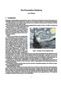
Figure 1: An example automatically-generated 3D bedroom scene rendered (top left) as a photorealistic RGB image with (top right) per-pixel ground truth of surface depth, surface normal, and object identity. The generated scenes include fine details: object textures (e.g., the duvet and pillow on the bed) are changeable, the materials of each object are sampled from actual physical parameters (reflectance, roughness, glossiness, etc.), and illumination parameters are sampled from continuous spaces of possible positions, intensities, and colors. Two additional room scene examples (bottom). Object models are from ShapeNet [10] and SUNCG [73].

1. Introduction Recent advances in recognition and classification through machine learning have yielded similar or even better performance than human abilities (e.g., [30, 18]) by leveraging large-scale, labeled RGB datasets [15, 46]. By contrast, the challenge of indoor scene understanding remains largely unsolved due in part to the limitations 1

of structured RGB-D datasets available for training. To address this problem, researchers have started collecting RGB-D imagery using Kinect-like sensors and preparing the associated ground truth data [71, 34]. However, the manual labeling of per-pixel ground truth information is tedious and error-prone, limiting its quantity and accuracy. In this paper, we propose a pipeline for the automatic synthesis of massive quantities of photorealistic images of indoor scenes. A stochastic grammar model, represented by a spatial attributed And-Or graph, which combines hierarchical compositions and contextual constraints, enables the systematic generation of 3D scenes with high variability. To avoid excessively dense graphs, our graphs utilize address nodes, resulting in a compact and meaningful representation. Using our easily configurable pipeline, we can systematically sample an infinite variety of illumination conditions (intensity, color, positions, etc.), camera parameters (Kinect, fisheye, panorama, depth of field, etc.), and object properties (geometry, color, texture, reflectance, roughness, glossiness, etc.). As Fig. 1 shows, we employ state-of-the-art physicsbased rendering, resulting in synthesized images with an impressive level of photorealism. Since our synthetic data is generated in a forward manner—by rendering 2D images from 3D scenes of known geometric object models— ground truth information is naturally available without any additional labeling. Hence, not only are our rendered images highly realistic, but they are also accompanied by perpixel ground truth color, depth, surface normals, and object labels. We demonstrate that our synthesized scenes achieve a performance similar to the NYU v2 Dataset on pre-trained deep learning models. By modifying pipeline components in a controllable manner, we furthermore provide diagnostics on common scene understanding tasks; e.g., depth and surface normal prediction, semantic segmentation, etc.

jects are pre-specified and remain the same. In comparison, we sample indoor scenes from scratch, and objects can be sampled. Some work studied fine-grained room arrangement to address specific problems; e.g., utilizing userprovided examples to arrange small objects [19, 91], and optimizing the number of objects in scenes using LARJMCMC [88]. To enhance realism, Merrell et al. [56] developed an interactive system that provides suggestions according to interior design guidelines. Image synthesis has been attempted using various deep neural network architectures, including recurrent neural networks (RNN) [23], generative adversarial networks (GAN) [80, 65], inverse graphics networks [42], and generative convolutional networks [53, 86, 85]. However, images of indoor scenes synthesized by these models often suffer from notable artifacts, such as undesirable blurred patches. More recently, some applications of general purpose inverse graphics solutions using probabilistic programming languages have been reported [55, 52, 41]. However, the problem space is enormous, and the quality of inverse graphics “renderings” is disappointingly low and slow. Stochastic scene grammar models have been used in computer vision to recover 3D structures from single-view images for both indoor [93, 49] and outdoor [49] scene parsing. In this paper, instead of solving inverse (vision) problems, we sample from the grammar model to generate, in a forward manner, large varieties of 3D indoor scenes.

1.1. Related Work

2.

Synthetic image datasets have recently been a source of training data for object detection and correspondence matching [77, 72, 96, 63], single-view reconstruction [35], pose estimation [70, 76, 87, 12], depth prediction [75], semantic segmentation [67], scene understanding [27, 37, 26], and in benchmark datasets [28]. Previously, synthetic imagery, generated on the fly, was used in visual surveillance [64] and active vision [78]. Although prior work demonstrates the potential of synthetic imagery to advance computer vision research, to our knowledge no large synthetic RGB-D dataset of indoor scenes has yet been released. 3D room synthesis algorithms [90, 27] have been developed to optimize furniture arrangements based on predefined constraints, where the number and categories of ob-

1.2. Contributions 1.

3.

4.

This paper makes five major contributions: To our knowledge, this is the first paper that, for the purposes of scene understanding, introduces a configurable pipeline to generate massive quantities of photorealistic images of indoor scenes with perfect per-pixel ground truth, including color, surface depth, surface normal, and object identity. To our knowledge, this is the first paper to utilize a stateof-the-art computer graphics rendering method, specifically physics-based ray tracing, to synthesize photorealistic images of remarkable quality for use in computer vision. By precisely customizing and controlling important attributes of the generated scenes, we provide a set of diagnostics benchmarks of previous work on several common computer vision tasks. To our knowledge, this is the first paper to provide comprehensive diagnostics with respect to algorithm stability and sensitivity to certain scene attributes. We propose a spatial attributed And-Or graph for scene layout generation. Our framework supports arbitrary addition and deletion of objects and modification of their categories, yielding significant variations in the resulting scene collection.

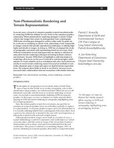
Figure 2: Scene grammar as an attributed S-AOG. The terminal nodes of the S-AOG are attributed with internal attributes (sizes) and external attributes (positions and orientations). A supported object node is combined by an address terminal node and a regular terminal node, indicating that the object is supported by the furniture pointed to by the address node. If the value of the address node is null, the object is situated on the floor. Contextual relations are defined between walls and furniture, among different furniture, between supported objects and supporting furniture, and for functional groups. 5. We demonstrate that the generated scenes achieves similar performance to the NYU v2 Dataset on pre-trained models, which indicates the high quality of our images.

2. Representation and Formulation 2.1. Attributed Spatial And-Or Graph In this section, we describe the model proposed to represent an indoor scene. A scene model should be capable of: i) representing the compositional/hierarchical structure of indoor scenes, and ii) capturing the rich contextual relationships between different components of the scene. An indoor scene can be first categorized into different indoor settings (i.e. bedrooms, bathrooms, etc.), each of which has a set of walls, furniture, and supported objects. Furniture can be decomposed into functional groups that are composed of multiple furniture, e.g. a “work” functional group consists of a desk and a chair. We consider four types of contextual relations: i) relations between furniture and walls; ii) relations among furniture; iii) relations between supported objects and their supporting objects (e.g., monitor and desk); and iv) relations between objects of a functional pair (e.g., sofa and TV). As shown in Fig. 2, we represent the hierarchical structure of indoor scenes by an attributed Spatial And-Or Graph (S-AOG), which is a Stochastic Context Sensitive Grammar (SCSG) with attributes on the terminal nodes. It combines i) a stochastic context free grammar (SCFG) and ii) contextual relations defined on a Markov random field (MRF); i.e., the horizontal links among the terminal nodes. The S-AOG represents the hierarchical decompositions from scenes (top level) to objects (bottom level) , whereas contextual rela-

tions encode the spatial and functional relations through horizontal links between nodes. An S-AOG is denoted by a 5-tuple: G = hS, V, R, P, Ei, where S is the root node of the grammar, V = VNT ∪ VT is the vertex set including non-terminal nodes VNT and terminal nodes VT , R stands for the production rules, P represents the probability model defined on the attributed SAOG, and E denotes the contextual relations represented as horizontal links between nodes in the same layer. The set of non-terminal nodes VNT = V And ∪ V Or ∪ Set V is composed of three set of nodes: And-nodes V And denoting a decomposition of a large entity, Ornodes V Or representing alternative decompositions, and Set-nodes V Set of which each child branch represents an Or-node on the number of the child object. The Set-nodes are compact representations of nested And-Or relations Correspondingly, three types of production rules are defined. i) And rules for an And-node v ∈ V And , are defined as a deterministic decomposition v → u1 · u2 · · · un(v) . ii) Or rules for an Or-node v ∈ V Or , are defined as a switch v → u1 |u2 · · · |un(v) with ρ1 |ρ2 · · · |ρn(v) . iii) Set rules for a Set-node v ∈ V Set , are defined as with v → (nil|u11 |u21 | · · · ) · · · (nil|u1n(v) |u2n(v) | · · · ), (ρ1,0 |ρ1,1 |ρ1,2 | · · · ) · · · (ρn(v),0 |ρn(v),1 |ρn(v),2 | · · · ), where uki denotes the case that object ui appears k times, and the probability is ρi,k . The set of terminal nodes can be divided into two types: i) regular terminal nodes v ∈ VTr representing spatial entities in a scene, with attributes A divided into internal Ain (size) and external Aex (position and orientation) attributes. ii) Address terminal nodes v ∈ VTa as pointers to regular ter-

minal nodes and takes values in the set VTr ∪ {nil}. These nodes avoid excessively dense graphs by encoding interactions that occur only in a certain context and are absent in all others [21]. Contextual Relations E = Ew ∪ Ef ∪ Eo ∪ Eg among nodes are represented by horizontal links in the AOG. The relations are divided into four subsets: i) relations between furniture and walls Ew ; ii) relations among furniture Ef ; iii) relations between supported objects and their supporting objects Eo (e.g., monitor and desk); and iv) relations between objects of a functional pair Eg (e.g., sofa and TV). Accordingly, the cliques formed in the terminal layer may also be divided into four subsets: C = Cw ∪ Cf ∪ Co ∪ Cg . Note that the contextual relations of nodes will be inherited from their parents; hence, the relations at a higher level will eventually collapse into cliques C among the terminal nodes. These contextual relations also form an MRF on the terminal nodes. To encode the contextual relations, we define different types of potential functions for different kinds of cliques. A hierarchical parse tree pt instantiates the S-AOG by selecting a child node for the Or-nodes as well as determining the state of each child node for the Set-nodes. A parse graph pg consists of a parse tree pt and a number of contextual relations E on the parse tree: pg = (pt, Ept ). Fig. 3 illustrates a simple example of a parse graph and four types of cliques formed in the terminal layer.

2.2. Probabilistic Formulation The purpose of the S-AOG is to generate realistic scene configurations from a learned S-AOG. Here we define the prior probability of a scene configuration generated by an S-AOG with the parameters Θ. A scene configuration is represented by a parse graph pg, including objects in the scene and their attributes. The prior probability of pg generated by an S-AOG parameterized by Θ is formulated as a Gibbs distribution: 1 p(pg|Θ) = exp{−E(pg|Θ)} Z 1 = exp{−E(pt|Θ) − E(Ept |Θ)}, Z

(1) (2)

where E(pg|Θ) is the energy function of a parse graph, E(pt|Θ) is the energy function of a parse tree, and E(Ept |Θ) is the energy term of the contextual relations. Here, the energy function of a parse tree is defined as combinations of probability distributions with closed-form expressions, and the energy of the contextual relations E is defined as potential functions relating to the external attributes of the terminal nodes. Energy E(pt|Θ) is further decomposed into energy functions of different types of non-terminal nodes, and energy functions of internal attributes of both regular and address terminal nodes:

Figure 3: (a) A simplified example of a parse graph of a bedroom. The terminal nodes of the parse graph form a MRF in the bottom layer. Cliques are formed by the contextual relations projected to the bottom layer. (b)-(e) give an example of the four types of cliques, which represent different contextual relations. E(pt|Θ) =

X

Or EΘ (v) +

v∈V Or

|

X

Set EΘ (v) +

v∈V Set

{z

non-terminal nodes

}

X

Ain EΘ (v),

v∈VTr

|

{z

terminal nodes

(3)

}

where the choice of child node of an Or-node v ∈ V Or follows a multinomial distribution, and each child branch of a Set-Note v ∈ V Set follows a Bernoulli distribution. Note that the And-nodes are deterministically expanded; hence, (3) lacks an energy term for the And-nodes. The internal attributes Ain (size) of terminal nodes follows a nonparametric probability distribution learned via kernel density estimation. The probability distribution 1 exp{−E(Ept |Θ)} Z Y Y Y Y = φw (c) φf (c) φo (c) φg (c)

p(Ept |Θ) =

c∈Cw

c∈Cf

c∈Co

(4) (5)

c∈Cg

combines the potentials of the four types of cliques formed

in the terminal layer, which are computed based on the external attributes of regular terminal nodes: • Potential function φw (c) is defined on relations between walls and furniture (Fig. 3(b)). A clique c ∈ Cw includes a terminal node representing a piece of furniture f and the terminal nodes representing walls {wi }: c = {f, {wi }}. Assuming pairwise object relations, φw (c) =

X 1 exp{ − lcon (wi , wj ) Z wi 6=wj | {z } −

wi

|

[ldis (f, wi ) + lori (f, wi )]}, {z

constraint between walls and furniture

(6)

}

where the cost function lcon (wi , wj ) defines the consistency between the walls; i.e., adjacent walls should be connected, whereas opposite walls should have the same size. Although this term is repeatedly computed in different cliques, it is usually zero as the walls are enforced to be consistent in practice. The cost function is ¯ i , xj )|, where defined as ldis (x1 , x − 2) = |d(xi , xj ) − d(x d(xi , xj ) is the distance between object xi and xj , and ¯ i , xj ) is the mean distance learned from examples. d(x The cost function lori (x1 , x − 2) = |θ(xi , xj ) − θ(xi¯, xj )| defines the incompatibility in terms of the relative orientations between two objects. • Potential function φf (c) is defined on relations between furniture (Fig. 3(c)). A clique c ∈ Cf includes all the terminal nodes representing a piece of furniture: c = {fi }. Hence, φf (c) =

X 1 exp{− locc (fi , fj )}, Z

(7)

fi 6=fj

X 1 exp{− (ldis (fig , fjg ) + lori (fig , fjg ))}. Z g g

(9)

fi 6=fj

1 exp{−lpos (f, o) − lori (f, o) − E add (a)}, Z

In this section, we introduce the learning algorithm for learning parameters of the S-AOG, and the sampling algorithm based on the learned S-AOG for synthesizing realistic scene configurations.

3.1. Learning We introduce how the probability model P of the S-AOG is learned in this section. From a set of annotated parse trees {pt m , m = 1, 2, · · · , M }, we can learn the branching probabilities ρ by maximum likelihood estimation (MLE). The MLE of the branching probabilities of Or-nodes and address terminal nodes is simply the frequency of each alternative choice [97]. However, the samples will not cover all possible terminal nodes to which an address node is pointing. There are many unseen but plausible configurations: e.g., an apple can be put on the chair, even though the examples might not cover this case. Inspired by the Dirichlet process, we address this issue by altering the MLE to include a small probability α for all branches: ρi =

#(v → ui ) + α

n(v) P j=1

where the cost function locc (fi , fj ) = max(0, 1 − d(fi , fj )/dacc ) defines the compatibility of two pieces of furniture in terms of occluding accessible space. • Potential function φo (c) is defined on relations between a supported object and the furniture that supports it (Fig. 3(d)). A clique c ∈ Co consists of a supported object terminal node o, the address node a connected to the object, and the furniture terminal node f pointed to by the address node: c = {f, a, o}. φo (c) =

φg (c) =

3. Learning, Sampling and Synthesis

constraint between walls

X

• Potential function φg (c) is defined for furniture in the same functional group (Fig. 3(d)). A clique c ∈ Cg consists of terminal nodes representing furniture in a functional group g: c = {fig }:

(8)

P where the cost function lpos (f, o) = i ldis (ffacei , o) defines the relative position of the supported object o to the four boundaries of the bounding box of the supporting furniture f . The energy term E add (a) is derived from the probability of an address node v ∈ VTa , which is regarded as a certain regular terminal node and follows a multinomial distribution.

.

(10)

(#(v → uj ) + α)

Similarly, for each child branch of the Set-nodes, we use the frequency in samples as the probability if it is non-zero, otherwise the probability to be turned on is α. In practice, we choose α to be 1, according to the standard practice of choosing the probability of joining a new table in the Chinese restaurant process [1]. The distribution of object size among all the furniture and supported objects is learned from the 3D models provided by ShapeNet [9] and SUNCG [73]. We first extracted the size information from the 3D models, and then fitted a non-parametric distribution using kernel density estimation (KDE). Not only is this more accurate than simply fitting a trivariate normal distribution, but it is also easier to sample from. The parameters of the potential functions are learned from the constructed scenes by computing the statistics of relative distances and relative orientations between different objects.

(a) β = 10.

(b) β = 100.

(c) β = 1000.

(d) β = 10000.

Figure 4: Synthesis for different values of β. Each image shows a typical configuration sampled from a Markov chain.

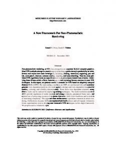
(a) Lighting intensity: half and double

(b) Lighting color: purple and blue

(c) Different object materials: metal, gold, chocolate, and clay

(d) Panorama image

(e) Video frames

(f) SLAM result

Figure 5: We can customize the scene with different (a) illumination intensities, (b) illumination colors, (c) materials, light source positions, camera lenses, and depths of field. We can also render the scene as (d) a panorama image or (e) a video. (f) SLAM reconstruction [81] result from the video in (e).

3.2. Sampling Scene Configurations Based on the learned S-AOG, we sample scene configurations (parse graphs) based on the prior probability p(pg|Θ) using a Markov Chain Monte Carlo (MCMC) sampler. The sampling process can be divided into two major steps: i) top-down sampling of the parse tree structure pt and internal attributes of objects by selecting a branch for Or-nodes and child branches for Set-nodes, and sampling the internal attributes (sizes) of each regular terminal node. Note that this can be easily done by sampling from closed-form distributions. ii) MCMC sampling of the exter-

nal attributes (positions and orientations) of objects as well as the values of the address nodes. Samples are proposed by Markov chain dynamics, and are taken after the Markov chain converges to the prior probability. These attributes are constrained by multiple potential functions, hence it is difficult to directly sample from the true underlying probability distribution. Four types of Markov chain dynamics qi , i = 1, 2, 3, 4 are designed to be chosen randomly with probabilities to propose moves. The dynamics q1 and q2 are diffusion, and q3 and q4 are reversible jumps: • Dynamic q1 (translation of objects) chooses a regular ter-

minal node and samples a new position based on the current position of the object: pos → pos + δpos, where δpos follows a bivariate normal distribution. • Dynamic q2 (rotation of objects) chooses a regular terminal node and samples a new orientation based on the current orientation of the object: θ → θ + δθ, where δθ follows a normal distribution. • Dynamic q3 (swapping of objects) chooses two regular terminal nodes and swaps the positions and orientations of the objects. • Dynamic q4 (swapping of supporting objects) chooses an address terminal node and samples a new regular furniture terminal node pointed to. Then, we sample a new location for the supported object: randomly sample x = ux ∗ wp and y = uy ∗ lp , where ux , uy ∼ unif(0, 1), and wp and lp are the width and length of the supporting object. The z value is simply the height of the supporting object. Adopting the Metropolis-Hastings algorithm, the newly proposed parse graph pg 0 is accepted according to the following acceptance probability: p(pg 0 |Θ)p(pg|pg 0 ) ) (11) p(pg|Θ)p(pg 0 |pg) p(pg 0 |Θ) = min(1, ) (12) p(pg|Θ) = min(1, exp(E(pg|Θ) − E(pg 0 |Θ))), (13)

α(pg 0 |pg, Θ) = min(1,

The proposal probabilities are canceled since the proposed moves are symmetric in probability. During the sampling process, a typical state is drawn from the distribution. We can easily control the tidiness of the sampled scenes by adding an extra parameter β to control the landscape of the prior distribution p(pg|Θ) = 1 Z exp{−βE(pg|Θ)}, and simulating a Markov chain under one specific β.

3.3. Scene Instantiation from Scene Layout Given a generated scene layout, the 3D scene is instantiated by assembling objects into it. We use ShapeNet [10] and SUNCG [73] as our 3D model dataset. Scene instantiation comprises five steps: i) Align orientations of the models based on the up vector defined in the dataset. ii) Given an object category defined in the scene layout, search all the 3D object models to find the model that best matches the length/width ratio. iii) Transform the object to the desired positions, orientations and scales according to the generated scene layout. iv) Since we fit only the length and width in Step ii, an extra step to adjust object position along the gravity direction is needed, resulting in no floating objects. v) Add the floor, walls, and ceiling to complete the instantiated scene.

3.4. Configurable scene synthesis As we generate scenes in a forward fashion, our pipeline enables the precise customization and control of important attributes of the generated scenes. Some configurations are shown in Fig. 5. The rendered images are determined by combinations of the following three factors: i) Illuminations, including light source positions, intensities, colors, and the number of light sources. ii) Cameras, such as fisheye, panorama, and Kinect cameras, have different focal lengths and apertures, yielding dramatically different rendered images. Thanks to physics-based rendering, our pipeline can even control the F-stop and focal distance, resulting in different depths of field. iii) Different object materials and textures will have various properties, represented by roughness, metallicness, and reflectivity.

4. Photorealistic Scene Rendering. Physics-based rendering (PBR) [62] has become the industry standard in computer graphics applications in recent years, and has been widely adopted for both offline and real-time rendering. Unlike traditional rendering techniques where heuristic shaders are used to control how light is scattered by a surface, PBR simulates the physics of real-world light via computing the bidirectional scattering distribution function (BSDF) [5] of the surface. Following the law of conservation of energy, PBR solves the rendering equation for the total spectral radiance of an outgoing light in direction w from point x on a surface Lo (x, w) = Le (x, w) Z + fr (x, w0 , w)Li (x, w0 )(−w0 · n)dw0 , (14) Ω

where Lo is the outgoing light, Le is emitted light (from a light source), Ω is the unit hemisphere uniquely determined by x and its normal, fr is the bidirectional reflectance distribution function (BRDF), Li is the incoming light from direction w0 , w0 · n accounts for the attenuation of the incoming light. In path tracing, the rendering equation is often solved with the Monte Carlo methods. Through computing both the reflected and transmitted components of rays in a physically accurate way while conserving energies, PBR allows photorealistic rendering of shadows, reflections and refractions that capture unprecedented levels of detail compared to any other exisiting shading techniques. Note PBR describes a shading process and does not reply on how images are rasterized to the screen space. In this paper we use the Mantra® PBR engine to render synthetic image data with raytracing for its accurate calculation of lighting and shading, as well as physically intuitive parameter configuration. Indoor scenes are typically closed rooms. Various reflective and diffusive surfaces may exist throughtout the space.

(a)

(b)

(c)

(d)

(e)

(f)

(g)

(h)

Figure 6: Benchmark results. (a) Given a set of generated RGB images rendered with different illuminations and object material properties (top to bottom: original settings, with high illumination, with blue illumination, with metallic material properties), we evaluate (b)–(d) three depth prediction algorithms, (e)–(f) two surface normal estimation algorithms, (g) a semantic segmentation algorithm, and (h) an object detection algorithm. Therefore the effect of secondary rays is particularly important for achiving realistic lighting. PBR robustly samples both direct lighting contribution from light sources and indirect lighting from diffused and reflected rays on surfaces. The BSDF shader on a surface manages and modifies its color contribution when hit by a secondary ray. Doing so results in more secondary rays being sent out from the surface in evaluation. The reflect limit (number of times a ray can be reflected) and the diffuse limit (number of times diffuse rays bounce on surfaces) need to be chosen wisely for balancing final image quality and render time. We found that a reflect limit of 10 and a diffuse limit of 4 gives visually plausible result with moderate computational cost.

Table 1: Depth estimation. Intensity, color, and material represent the scene with different illumination intensities, colors, and object material properties, respectively. Setting Origin Intensity Color Material

Method [47] [17] [16] [47] [17] [16] [47] [17] [16] [47] [17] [16]

Abs Rel 0.225 0.373 0.366 0.216 0.483 0.457 0.332 0.509 0.491 0.192 0.395 0.393

Sqr Rel 0.146 0.358 0.347 0.165 0.511 0.469 0.304 0.540 0.508 0.130 0.389 0.395

Error Log10 RMSE(linear) 0.089 0.585 0.147 0.802 0.171 0.910 0.085 0.561 0.183 0.930 0.201 1.01 0.113 0.643 0.190 0.923 0.203 0.961 0.08 0.534 0.155 0.823 0.169 0.882

RMSE(log) 0.117 0.191 0.206 0.118 0.24 0.217 0.166 0.239 0.247 0.106 0.199 0.209

δ < 1.25 0.642 0.367 0.287 0.683 0.205 0.284 0.582 0.263 0.241 0.693 0.345 0.291

Accuracy δ < 1.252 δ < 1.253 0.914 0.987 0.745 0.924 0.617 0.863 0.915 0.971 0.551 0.802 0.607 0.851 0.852 0.928 0.592 0.851 0.531 0.806 0.930 0.985 0.709 0.908 0.631 0.889

5. Evaluation Results To learn the S-AOG, we annotated parse graphs for part of the SUNCG [73] indoor scenes according to the attributed S-AOG structure shown in Fig. 2. We obtained object labels from ShapeNetSem [10] (a subset of ShapeNet annotated with physical attributes) and SUNCG [73]. The objects are classified into two classes: furniture and supported objects. We annotated the set of furniture Fs and supported objects Os that appear in each scene as well as the functional groups. To evaluate the generated indoor scenes, we selected common scene understanding tasks with state-of-the-art alTable 2: Surface Normal Estimation. Intensity, color and material represent the setting with different illumination intensities, illumination colors, and object material properties.

Setting Origin Intensity Color Material

Method [16] [2] [16] [2] [16] [2] [16] [2]

Mean 22.74 24.45 24.15 24.20 26.53 27.11 22.86 24.15

Error Median 13.82 16.49 14.92 16.70 17.18 18.65 15.33 16.76

RMSE 32.48 33.07 33.53 32.29 36.36 35.67 32.62 32.24

11.25◦ 43.34 35.18 39.23 32.00 34.20 28.19 36.99 33.52

Accuracy 22.5◦ 67.64 61.69 66.04 62.56 60.33 58.23 65.21 62.50

30◦ 75.51 70.85 73.86 72.22 70.46 68.31 73.31 72.17

Figure 7: Qualitative results in different types of scenes. gorithms as a benchmark under various different environments, which evaluates the algorithms’ stabilities and sensitivities. Moreover, it also reveals the potentials of training large-scale scene understanding algorithms with the proposed dataset. Depth Estimation. We evaluated three state-of-the-art algorithms for single-image depth estimation: Eigens et al. [17, 16] and Liu et al. [47]. Table. 1 presents a quantitative comparison. We see that [17, 16] are very sensitive to illumination condition, whereas [47] is robust to illumination intensity, but sensitive to illumination color. In addition, all three algorithms are robust to different object materials. This may be because material changes do not alter the continuity of the surface. Note that [48] exhibits nearly the same performance on both our dataset and the NYU v2 Dataset, which indicates that our synthetic scenes are suitable for algorithm evaluation. Surface Normal Estimation. We evaluated two surface normal estimation algorithms: Eigens et al. [16] and Bansal et al. [2]. Table. 2 shows the quantitative results. Compared with depth estimation, the surface normal estimation algorithms are stable to different illumination conditions as well as to different material properties. The two algorithms achieve comparable results on the NYU Dataset. Semantic Segmentation. We applied the semantic segmentation model in [16]. Since we have 129 classes of indoor objects whereas the model only has a maximum of 40 classes, we re-arranged and reduced the number of classes to fit the prediction of the model. The algorithm achieves 60.5 pixel accuracy and 50.4 mIoU on our dataset. 3D Reconstructions. ElasticFusion [81] is evaluated given a set of images generated by our pipeline. A qualitative result is shown in Fig. 5f. Object Detection. We apply the Faster R-CNN Model [66] to detect objects. We again needed to re-arrange and reduce the number of classes for evaluation. Because there are only a few overlapping object classes between our synthetic scenes and the published output of the algorithm, Fig. 6 shows only qualitative results. A model trained on our dataset is needed for further evaluation.

6. Conclusion and Future Work The proposed pipeline to generate configurable room layouts can provide detailed ground truth for supervised training. We believe such capability of generating room layouts in a controllable manner can benefit various vision areas, including but not limited to depth prediction [17, 16, 47, 43], surface normal prediction [79, 16, 2], semantic segmentation [51, 59, 11], reasoning about object-supporting relations [20, 71, 94, 45], material recognition [7, 6, 8, 83], recovery of illumination conditions [58, 69, 40, 60, 4, 29, 92, 61, 50], inferring room layout and scene parsing [33, 31, 44, 24, 14, 84, 93, 54, 13], object functionality and affordance [74, 3, 22, 32, 93, 25, 36, 98, 57, 38, 89, 39, 68] and physics reasoning [95, 94, 100, 83, 99, 82]. In additional, we believe that research on 3D reconstruction in robotics and on the psychophysics of human perception can also benefit from our work. Our current approach has several limitations that we will address in future research: first, the scene generation process can be improved with a multi-stage sampling process; i.e., sampling large furniture first and smaller objects later, which can potentially improve the scene layout. Second, we shall consider human activity inside the generated scene, especially functionality and affordance. Adding virtual humans into the scenes can provide additional ground truth for human pose recognition, human tracking, etc.

References ´ [1] D. J. Aldous. Exchangeability and related topics. In Ecole ´ e de Probabilités de Saint-Flour XIII1983, pages 1– d’Et´ 198. Springer, 1985. 5 [2] A. Bansal, B. Russell, and A. Gupta. Marr revisited: 2d3d alignment via surface normal prediction. arXiv preprint arXiv:1604.01347, 2016. 8, 9 [3] E. Bar-Aviv and E. Rivlin. Functional 3d object classification using simulation of embodied agent. In British Machine Vision Conference (BMVC), 2006. 9 [4] J. T. Barron and J. Malik. Shape, illumination, and reflectance from shading. Transactions on Pattern Analysis and Machine Intelligence (TPAMI), 37(8), 2015. 9

[5] F. O. Bartell, E. L. Dereniak, and W. L. Wolfe. The theory and measurement of bidirectional reflectance distribution function (brdf) and bidirectional transmittance distribution function (btdf), 1981. 7 [6] S. Bell, K. Bala, and N. Snavely. Intrinsic images in the wild. ACM Transactions on Graphics (TOG), 33(4), 2014. 9 [7] S. Bell, P. Upchurch, N. Snavely, and K. Bala. Opensurfaces: A richly annotated catalog of surface appearance. ACM Transactions on Graphics (TOG), 32(4), 2013. 9 [8] S. Bell, P. Upchurch, N. Snavely, and K. Bala. Material recognition in the wild with the materials in context database. In Conference on Computer Vision and Pattern Recognition (CVPR), 2015. 9 [9] A. X. Chang, T. Funkhouser, L. Guibas, P. Hanrahan, Q. Huang, Z. Li, S. Savarese, M. Savva, S. Song, H. Su, et al. Shapenet: An information-rich 3d model repository. arXiv preprint arXiv:1512.03012, 2015. 5 [10] A. X. Chang, T. Funkhouser, L. Guibas, P. Hanrahan, Q. Huang, Z. Li, S. Savarese, M. Savva, S. Song, H. Su, J. Xiao, L. Yi, and F. Yu. ShapeNet: An Information-Rich 3D Model Repository. arXiv preprint arXiv:1512.03012, 2015. 1, 7, 8 [11] L.-C. Chen, G. Papandreou, I. Kokkinos, K. Murphy, and A. L. Yuille. Deeplab: Semantic image segmentation with deep convolutional nets, atrous convolution, and fully connected crfs. arXiv preprint arXiv:1606.00915, 2016. 9 [12] W. Chen, H. Wang, Y. Li, H. Su, D. Lischinsk, D. CohenOr, B. Chen, et al. Synthesizing training images for boosting human 3d pose estimation. In International Conference on 3D Vision (3DV), 2016. 2 [13] W. Choi, Y.-W. Chao, C. Pantofaru, and S. Savarese. Indoor scene understanding with geometric and semantic contexts. International Journal of Computer Vision (IJCV), 112(2), 2015. 9 [14] L. Del Pero, J. Bowdish, D. Fried, B. Kermgard, E. Hartley, and K. Barnard. Bayesian geometric modeling of indoor scenes. In Conference on Computer Vision and Pattern Recognition (CVPR), 2012. 9 [15] J. Deng, W. Dong, R. Socher, L.-J. Li, K. Li, and L. FeiFei. Imagenet: A large-scale hierarchical image database. In Conference on Computer Vision and Pattern Recognition (CVPR), 2009. 1 [16] D. Eigen and R. Fergus. Predicting depth, surface normals and semantic labels with a common multi-scale convolutional architecture. In International Conference on Computer Vision (ICCV), 2015. 8, 9 [17] D. Eigen, C. Puhrsch, and R. Fergus. Depth map prediction from a single image using a multi-scale deep network. In Advances in Neural Information Processing Systems (NIPS), 2014. 8, 9 [18] M. Everingham, S. A. Eslami, L. Van Gool, C. K. Williams, J. Winn, and A. Zisserman. The pascal visual object classes challenge: A retrospective. International Journal of Computer Vision (IJCV), 111(1), 2015. 1 [19] M. Fisher, D. Ritchie, M. Savva, T. Funkhouser, and P. Hanrahan. Example-based synthesis of 3d object arrangements. ACM Transactions on Graphics (TOG), 31(6), 2012. 2

[20] M. Fisher, M. Savva, and P. Hanrahan. Characterizing structural relationships in scenes using graph kernels. ACM Transactions on Graphics (TOG), 30(4), 2011. 9 [21] A. Fridman. Mixed markov models. Proceedings of the National Academy of Sciences (PNAS), 100(14), 2003. 4 [22] H. Grabner, J. Gall, and L. Van Gool. What makes a chair a chair? In Conference on Computer Vision and Pattern Recognition (CVPR), 2011. 9 [23] K. Gregor, I. Danihelka, A. Graves, D. J. Rezende, and D. Wierstra. Draw: A recurrent neural network for image generation. arXiv preprint arXiv:1502.04623, 2015. 2 [24] A. Gupta, M. Hebert, T. Kanade, and D. M. Blei. Estimating spatial layout of rooms using volumetric reasoning about objects and surfaces. In Advances in Neural Information Processing Systems (NIPS), 2010. 9 [25] A. Gupta, S. Satkin, A. A. Efros, and M. Hebert. From 3d scene geometry to human workspace. In Conference on Computer Vision and Pattern Recognition (CVPR), 2011. 9 [26] A. Handa, V. P˘atr˘aucean, V. Badrinarayanan, S. Stent, and R. Cipolla. Understanding real world indoor scenes with synthetic data. In Conference on Computer Vision and Pattern Recognition (CVPR), 2016. 2 [27] A. Handa, V. Patraucean, S. Stent, and R. Cipolla. Scenenet: an annotated model generator for indoor scene understanding. In International Conference on Robotics and Automation (ICRA), 2016. 2 [28] A. Handa, T. Whelan, J. McDonald, and A. J. Davison. A benchmark for rgb-d visual odometry, 3d reconstruction and slam. In International Conference on Robotics and Automation (ICRA), 2014. 2 [29] K. Hara, K. Nishino, et al. Light source position and reflectance estimation from a single view without the distant illumination assumption. Transactions on Pattern Analysis and Machine Intelligence (TPAMI), 27(4), 2005. 9 [30] K. He, X. Zhang, S. Ren, and J. Sun. Delving deep into rectifiers: Surpassing human-level performance on imagenet classification. In International Conference on Computer Vision (ICCV), 2015. 1 [31] V. Hedau, D. Hoiem, and D. Forsyth. Recovering the spatial layout of cluttered rooms. In International Conference on Computer Vision (ICCV), 2009. 9 [32] T. Hermans, J. M. Rehg, and A. Bobick. Affordance prediction via learned object attributes. In International Conference on Robotics and Automation (ICRA), 2011. 9 [33] D. Hoiem, A. A. Efros, and M. Hebert. Automatic photo pop-up. ACM Transactions on Graphics (TOG), 24(3), 2005. 9 [34] B.-S. Hua, Q.-H. Pham, D. T. Nguyen, M.-K. Tran, L.-F. Yu, and S.-K. Yeung. Scenenn: A scene meshes dataset with annotations. In International Conference on 3D Vision (3DV), 2016. 2 [35] Q. Huang, H. Wang, and V. Koltun. Single-view reconstruction via joint analysis of image and shape collections. ACM Transactions on Graphics (TOG), 34(4), 2015. 2 [36] Y. Jiang, H. Koppula, and A. Saxena. Hallucinated humans as the hidden context for labeling 3d scenes. In Conference on Computer Vision and Pattern Recognition (CVPR), 2013. 9

[37] Y. Z. M. B. P. Kohli, S. Izadi, and J. Xiao. Deepcontext: Context-encoding neural pathways for 3d holistic scene understanding. arXiv preprint arXiv:1603.04922, 2016. 2 [38] H. S. Koppula and A. Saxena. Physically grounded spatiotemporal object affordances. In European Conference on Computer Vision (ECCV), 2014. 9 [39] H. S. Koppula and A. Saxena. Anticipating human activities using object affordances for reactive robotic response. Transactions on Pattern Analysis and Machine Intelligence (TPAMI), 38(1), 2016. 9 [40] L. Kratz and K. Nishino. Factorizing scene albedo and depth from a single foggy image. In International Conference on Computer Vision (ICCV), 2009. 9 [41] T. D. Kulkarni, P. Kohli, J. B. Tenenbaum, and V. Mansinghka. Picture: A probabilistic programming language for scene perception. In Conference on Computer Vision and Pattern Recognition (CVPR), 2015. 2 [42] T. D. Kulkarni, W. F. Whitney, P. Kohli, and J. Tenenbaum. Deep convolutional inverse graphics network. In Advances in Neural Information Processing Systems (NIPS), 2015. 2 [43] I. Laina, C. Rupprecht, V. Belagiannis, F. Tombari, and N. Navab. Deeper depth prediction with fully convolutional residual networks. arXiv preprint arXiv:1606.00373, 2016. 9 [44] D. C. Lee, M. Hebert, and T. Kanade. Geometric reasoning for single image structure recovery. In Conference on Computer Vision and Pattern Recognition (CVPR), 2009. 9 [45] W. Liang, Y. Zhao, Y. Zhu, and S.-C. Zhu. What is where: Inferring containment relations from videos. In International Joint Conference on Artificial Intelligence (IJCAI), 2016. 9 [46] T.-Y. Lin, M. Maire, S. Belongie, J. Hays, P. Perona, D. Ramanan, P. Dollár, and C. L. Zitnick. Microsoft coco: Common objects in context. In European Conference on Computer Vision (ECCV), 2014. 1 [47] F. Liu, C. Shen, and G. Lin. Deep convolutional neural fields for depth estimation from a single image. In Conference on Computer Vision and Pattern Recognition (CVPR), 2015. 8, 9 [48] T. Liu, S. Chaudhuri, V. G. Kim, Q. Huang, N. J. Mitra, and T. Funkhouser. Creating consistent scene graphs using a probabilistic grammar. ACM Transactions on Graphics (TOG), 33(6), 2014. 9 [49] X. Liu, Y. Zhao, and S.-C. Zhu. Single-view 3d scene parsing by attributed grammar. In Conference on Computer Vision and Pattern Recognition (CVPR), 2014. 2 [50] S. Lombardi and K. Nishino. Reflectance and illumination recovery in the wild. Transactions on Pattern Analysis and Machine Intelligence (TPAMI), 38(1), 2016. 9 [51] J. Long, E. Shelhamer, and T. Darrell. Fully convolutional networks for semantic segmentation. In Conference on Computer Vision and Pattern Recognition (CVPR), 2015. 9 [52] M. M. Loper and M. J. Black. Opendr: An approximate differentiable renderer. In European Conference on Computer Vision (ECCV), 2014. 2

[53] Y. Lu, S.-C. Zhu, and Y. N. Wu. Learning frame models using cnn filters. In AAAI Conference on Artificial Intelligence (AAAI), 2016. 2 [54] A. Mallya and S. Lazebnik. Learning informative edge maps for indoor scene layout prediction. In International Conference on Computer Vision (ICCV), 2015. 9 [55] V. Mansinghka, T. D. Kulkarni, Y. N. Perov, and J. Tenenbaum. Approximate bayesian image interpretation using generative probabilistic graphics programs. In Advances in Neural Information Processing Systems (NIPS), 2013. 2 [56] P. Merrell, E. Schkufza, Z. Li, M. Agrawala, and V. Koltun. Interactive furniture layout using interior design guidelines. ACM Transactions on Graphics (TOG), 30(4), 2011. 2 [57] A. Myers, A. Kanazawa, C. Fermuller, and Y. Aloimonos. Affordance of object parts from geometric features. In Workshop on Vision meets Cognition, CVPR, 2014. 9 [58] K. Nishino, Z. Zhang, and K. Ikeuchi. Determining reflectance parameters and illumination distribution from a sparse set of images for view-dependent image synthesis. In International Conference on Computer Vision (ICCV), 2001. 9 [59] H. Noh, S. Hong, and B. Han. Learning deconvolution network for semantic segmentation. In International Conference on Computer Vision (ICCV), 2015. 9 [60] G. Oxholm and K. Nishino. Multiview shape and reflectance from natural illumination. In Conference on Computer Vision and Pattern Recognition (CVPR), 2014. 9 [61] G. Oxholm and K. Nishino. Shape and reflectance estimation in the wild. Transactions on Pattern Analysis and Machine Intelligence (TPAMI), 38(2), 2016. 9 [62] M. Pharr and G. Humphreys. Physically based rendering: From theory to implementation. Morgan Kaufmann, 2004. 7 [63] C. R. Qi, H. Su, M. Niessner, A. Dai, M. Yan, and L. J. Guibas. Volumetric and multi-view cnns for object classification on 3d data. In Conference on Computer Vision and Pattern Recognition (CVPR), 2016. 2 [64] F. Qureshi and D. Terzopoulos. Smart camera networks in virtual reality. Proceedings of the IEEE, 96(10):1640–1656, 2008. 2 [65] A. Radford, L. Metz, and S. Chintala. Unsupervised representation learning with deep convolutional generative adversarial networks. arXiv preprint arXiv:1511.06434, 2015. 2 [66] S. Ren, K. He, R. Girshick, and J. Sun. Faster r-cnn: Towards real-time object detection with region proposal networks. In Advances in Neural Information Processing Systems (NIPS), 2015. 9 [67] S. R. Richter, V. Vineet, S. Roth, and V. Koltun. Playing for data: Ground truth from computer games. In European Conference on Computer Vision (ECCV), 2016. 2 [68] A. Roy and S. Todorovic. A multi-scale cnn for affordance segmentation in rgb images. In European Conference on Computer Vision (ECCV), 2016. 9 [69] I. Sato, Y. Sato, and K. Ikeuchi. Illumination from shadows. Transactions on Pattern Analysis and Machine Intelligence (TPAMI), 25(3), 2003. 9

[70] G. Shakhnarovich, P. Viola, and T. Darrell. Fast pose estimation with parameter-sensitive hashing. In International Conference on Computer Vision (ICCV), 2003. 2 [71] N. Silberman, D. Hoiem, P. Kohli, and R. Fergus. Indoor segmentation and support inference from rgbd images. In European Conference on Computer Vision (ECCV), 2012. 2, 9 [72] S. Song and J. Xiao. Sliding shapes for 3d object detection in depth images. In European Conference on Computer Vision (ECCV), 2014. 2 [73] S. Song, F. Yu, A. Zeng, A. X. Chang, M. Savva, and T. Funkhouser. Semantic scene completion from a single depth image. arXiv preprint arXiv:1611.08974, 2016. 1, 5, 7, 8 [74] L. Stark and K. Bowyer. Achieving generalized object recognition through reasoning about association of function to structure. Transactions on Pattern Analysis and Machine Intelligence (TPAMI), 13(10), 1991. 9 [75] H. Su, Q. Huang, N. J. Mitra, Y. Li, and L. Guibas. Estimating image depth using shape collections. ACM Transactions on Graphics (TOG), 33(4):37, 2014. 2 [76] H. Su, C. R. Qi, Y. Li, and L. J. Guibas. Render for cnn: Viewpoint estimation in images using cnns trained with rendered 3d model views. In International Conference on Computer Vision (ICCV), 2015. 2 [77] B. Sun and K. Saenko. From virtual to reality: Fast adaptation of virtual object detectors to real domains. In British Machine Vision Conference (BMVC), 2014. 2 [78] D. Terzopoulos and T. Rabie. Animat vision: Active vision in artificial animals. Videre: Journal of Computer Vision Research, 1(1):2–19, 1997. 2 [79] X. Wang, D. Fouhey, and A. Gupta. Designing deep networks for surface normal estimation. In Conference on Computer Vision and Pattern Recognition (CVPR), 2015. 9 [80] X. Wang and A. Gupta. Generative image modeling using style and structure adversarial networks. arXiv preprint arXiv:1603.05631, 2016. 2 [81] T. Whelan, S. Leutenegger, R. F. Salas-Moreno, B. Glocker, and A. J. Davison. Elasticfusion: Dense slam without a pose graph. In Robotics: Science and Systems (RSS), 2015. 6, 9 [82] J. Wu. Computational perception of physical object properties. PhD thesis, Massachusetts Institute of Technology, 2016. 9 [83] J. Wu, I. Yildirim, J. J. Lim, B. Freeman, and J. Tenenbaum. Galileo: Perceiving physical object properties by integrating a physics engine with deep learning. In Advances in Neural Information Processing Systems (NIPS), 2015. 9 [84] J. Xiao, B. Russell, and A. Torralba. Localizing 3d cuboids in single-view images. In Advances in Neural Information Processing Systems (NIPS), 2012. 9 [85] J. Xie, Y. Lu, S.-C. Zhu, and Y. N. Wu. Cooperative training of descriptor and generator networks. arXiv preprint arXiv:1609.09408, 2016. 2 [86] J. Xie, Y. Lu, S.-C. Zhu, and Y. N. Wu. A theory of generative convnet. In International Conference on Machine Learning (ICML), 2016. 2

[87] H. Yasin, U. Iqbal, B. Krüger, A. Weber, and J. Gall. A dual-source approach for 3d pose estimation from a single image. In Conference on Computer Vision and Pattern Recognition (CVPR), 2016. 2 [88] Y.-T. Yeh, L. Yang, M. Watson, N. D. Goodman, and P. Hanrahan. Synthesizing open worlds with constraints using locally annealed reversible jump mcmc. ACM Transactions on Graphics (TOG), 31(4), 2012. 2 [89] L.-F. Yu, N. Duncan, and S.-K. Yeung. Fill and transfer: A simple physics-based approach for containability reasoning. In International Conference on Computer Vision (ICCV), 2015. 9 [90] L. F. Yu, S. K. Yeung, C. K. Tang, D. Terzopoulos, T. F. Chan, and S. J. Osher. Make it home: automatic optimization of furniture arrangement. ACM Transactions on Graphics (TOG), 30(4), 2011. 2 [91] L.-F. Yu, S.-K. Yeung, and D. Terzopoulos. The clutterpalette: An interactive tool for detailing indoor scenes. IEEE transactions on visualization and computer graphics, 22(2):1138–1148, 2016. 2 [92] H. Zhang, K. Dana, and K. Nishino. Reflectance hashing for material recognition. In Conference on Computer Vision and Pattern Recognition (CVPR), 2015. 9 [93] Y. Zhao and S.-C. Zhu. Scene parsing by integrating function, geometry and appearance models. In Conference on Computer Vision and Pattern Recognition (CVPR), 2013. 2, 9 [94] B. Zheng, Y. Zhao, J. Yu, K. Ikeuchi, and S.-C. Zhu. Scene understanding by reasoning stability and safety. International Journal of Computer Vision (IJCV), 112(2), 2015. 9 [95] B. Zheng, Y. Zhao, J. C. Yu, K. Ikeuchi, and S.-C. Zhu. Beyond point clouds: Scene understanding by reasoning geometry and physics. In Conference on Computer Vision and Pattern Recognition (CVPR), 2013. 9 [96] T. Zhou, P. Krähenbühl, M. Aubry, Q. Huang, and A. A. Efros. Learning dense correspondence via 3d-guided cycle consistency. In Conference on Computer Vision and Pattern Recognition (CVPR), 2016. 2 [97] S.-C. Zhu and D. Mumford. A stochastic grammar of images. Now Publishers Inc, 2007. 5 [98] Y. Zhu, A. Fathi, and L. Fei-Fei. Reasoning about object affordances in a knowledge base representation. In European Conference on Computer Vision (ECCV), 2014. 9 [99] Y. Zhu, C. Jiang, Y. Zhao, D. Terzopoulos, and S.-C. Zhu. Inferring forces and learning human utilities from videos. In Conference on Computer Vision and Pattern Recognition (CVPR), 2016. 9 [100] Y. Zhu, Y. Zhao, and S.-C. Zhu. Understanding tools: Task-oriented object modeling, learning and recognition. In Conference on Computer Vision and Pattern Recognition (CVPR), 2015. 9

Supplementary Material

Figure 8: 10 Categories of Typical Scenes: bathroom, bedroom, dining room, garage, guestroom, gym, kitchen, living room, office, and storage room.

Figure 9: 100 Examples of RGB-D Images with Normal Map and Semantic Segmentation Ground Truth.

Figure 10: 100 Examples of RGB-D Images with Normal Map and Semantic Segmentation Ground Truth (Continue).














