Consistent Measurements of alpha_s from Precise Oriented Event ...

EUROPEAN ORGANIZATION FOR NUCLEAR RESEARCH CERN–EP/99-133

arXiv:hep-ex/0002026v1 8 Feb 2000

26 January 2000 revised

Consistent Measurements of αs from Precise Oriented Event Shape Distributions DELPHI Collaboration

Abstract √ An updated analysis using about 1.5 million events recorded at s = MZ with the DELPHI detector in 1994 is presented. Eighteen infrared and collinear safe event shape observables are measured as a function of the polar angle of the thrust axis. The data are compared to theoretical calculations in O(αs2 ) including the event orientation. A combined fit of αs and of the renormalization scale xµ in O(αs2 ) yields an excellent description of the high statistics data. The weighted average from 18 observables including quark mass effects and correlations is αs (M2Z ) = 0.1174±0.0026. The final result, derived from the jet cone energy fraction, the observable with the smallest theoretical and experimental uncertainty, is αs (M2Z ) = 0.1180 ± 0.0006(exp.) ± 0.0013(hadr.) ± 0.0008(scale) ± 0.0007(mass). Further studies include an αs determination using theoretical predictions in the next-to-leading log approximation (NLLA), matched NLLA and O(αs2 ) predictions as well as theoretically motivated optimized scale setting methods. The influence of higher order contributions was also investigated by using the method of Pad´e approximants. Average αs values derived from the different approaches are in good agreement.

(Submitted to E. Phys. J. C)

ii P.Abreu22 , W.Adam50 , T.Adye37 , P.Adzic11 , Z.Albrecht18 , T.Alderweireld2 , G.D.Alekseev17 , R.Alemany49 , T.Allmendinger18 , P.P.Allport23 , S.Almehed25 , U.Amaldi9 , N.Amapane45 , S.Amato47 , E.G.Anassontzis3 , P.Andersson44 , A.Andreazza9 , S.Andringa22 , P.Antilogus26 , W-D.Apel18 , Y.Arnoud9 , B.˚ Asman44 , 26 9 9 20 22 46 J-E.Augustin , A.Augustinus , P.Baillon , P.Bambade , F.Barao , G.Barbiellini , R.Barbier26 , D.Y.Bardin17 , G.Barker18 , A.Baroncelli39 , M.Battaglia16 , M.Baubillier24 , K-H.Becks52 , M.Begalli6 , A.Behrmann52 , P.Beilliere8 , Yu.Belokopytov9,53 , N.C.Benekos32 , A.C.Benvenuti5 , C.Berat15 , M.Berggren26 , D.Bertini26 , D.Bertrand2 , M.Besancon40 , M.Bigi45 , M.S.Bilenky17 , M-A.Bizouard20 , D.Bloch10 , H.M.Blom31 , M.Bonesini28 , W.Bonivento28 , M.Boonekamp40 , P.S.L.Booth23 , A.W.Borgland4 , G.Borisov20 , C.Bosio42 , O.Botner48 , E.Boudinov31 , B.Bouquet20 , C.Bourdarios20 , T.J.V.Bowcock23 , I.Boyko17 , I.Bozovic11 , M.Bozzo14 , P.Branchini39 , T.Brenke52 , R.A.Brenner48 , P.Bruckman19 , J-M.Brunet8 , L.Bugge33 , T.Buran33 , 52 50 52 49 28 28 T.Burgsmueller , B.Buschbeck , P.Buschmann , S.Cabrera , M.Caccia , M.Calvi , T.Camporesi9 , V.Canale38 , F.Carena9 , L.Carroll23 , C.Caso14 , M.V.Castillo Gimenez49 , A.Cattai9 , F.R.Cavallo5 , V.Chabaud9 , Ph.Charpentier9 , L.Chaussard26 , P.Checchia36 , G.A.Chelkov17 , R.Chierici45 , P.Chochula7 , V.Chorowicz26 , J.Chudoba30 , K.Cieslik19 , P.Collins9 , R.Contri14 , E.Cortina49 , G.Cosme20 , F.Cossutti9 , J-H.Cowell23 , H.B.Crawley1 , D.Crennell37 , S.Crepe15 , G.Crosetti14 , J.Cuevas Maestro34 , S.Czellar16 , M.Davenport9 , W.Da Silva24 , A.Deghorain2 , G.Della Ricca46 , P.Delpierre27 , N.Demaria9 , A.De Angelis9 , W.De Boer18 , C.De Clercq2 , B.De Lotto46 , A.De Min36 , L.De Paula47 , H.Dijkstra9 , L.Di Ciaccio38,9 , J.Dolbeau8 , K.Doroba51 , M.Dracos10 , J.Drees52 , M.Dris32 , A.Duperrin26 , J-D.Durand9 , G.Eigen4 , T.Ekelof48 , G.Ekspong44 , M.Ellert48 , M.Elsing9 , J-P.Engel10 , B.Erzen43 , M.Espirito Santo22 , G.Fanourakis11 , D.Fassouliotis11 , J.Fayot24 , M.Feindt18 , P.Ferrari28 , A.Ferrer49 , E.Ferrer-Ribas20 , F.Ferro14 , S.Fichet24 , A.Firestone1 , U.Flagmeyer52 , H.Foeth9 , E.Fokitis32 , F.Fontanelli14 , B.Franek37 , A.G.Frodesen4 , R.Fruhwirth50 , F.Fulda-Quenzer20 , J.Fuster49 , A.Galloni23 , D.Gamba45 , S.Gamblin20 , M.Gandelman47 , C.Garcia49 , C.Gaspar9 , M.Gaspar47 , U.Gasparini36 , Ph.Gavillet9 , E.N.Gazis32 , D.Gele10 , N.Ghodbane26 , I.Gil49 , F.Glege52 , R.Gokieli9,51 , B.Golob43 , G.Gomez-Ceballos41 , P.Goncalves22 , I.Gonzalez Caballero41 , G.Gopal37 , L.Gorn1,54 , V.Gracco14 , J.Grahl1 , E.Graziani39 , C.Green23 , H-J.Grimm18 , P.Gris40 , G.Grosdidier20 , K.Grzelak51 , M.Gunther48 , J.Guy37 , F.Hahn9 , S.Hahn52 , S.Haider9 , A.Hallgren48 , K.Hamacher52 , J.Hansen33 , F.J.Harris35 , V.Hedberg25 , S.Heising18 , J.J.Hernandez49 , P.Herquet2 , H.Herr9 , T.L.Hessing35 , J.-M.Heuser52 , E.Higon49 , S-O.Holmgren44 , P.J.Holt35 , S.Hoorelbeke2 , M.Houlden23 , J.Hrubec50 , K.Huet2 , G.J.Hughes23 , K.Hultqvist44 , J.N.Jackson23 , R.Jacobsson9 , P.Jalocha9 , R.Janik7 , Ch.Jarlskog25 , G.Jarlskog25 , P.Jarry40 , B.Jean-Marie20 , E.K.Johansson44 , P.Jonsson26 , C.Joram9 , P.Juillot10 , F.Kapusta24 , K.Karafasoulis11 , S.Katsanevas26 , E.C.Katsoufis32 , R.Keranen18 , B.P.Kersevan43 , B.A.Khomenko17 , N.N.Khovanski17 , A.Kiiskinen16 , B.King23 , A.Kinvig23 , N.J.Kjaer31 , O.Klapp52 , H.Klein9 , P.Kluit31 , P.Kokkinias11 , M.Koratzinos9 , C.Kourkoumelis3 , O.Kouznetsov40 , M.Krammer50 , E.Kriznic43 , Z.Krumstein17 , P.Kubinec7 , J.Kurowska51 , K.Kurvinen16 , J.W.Lamsa1 , D.W.Lane1 , P.Langefeld52 , J-P.Laugier40 , R.Lauhakangas16 , G.Leder50 , F.Ledroit15 , V.Lefebure2 , L.Leinonen44 , A.Leisos11 , R.Leitner30 , J.Lemonne2 , G.Lenzen52 , V.Lepeltier20 , T.Lesiak19 , M.Lethuillier40 , J.Libby35 , D.Liko9 , A.Lipniacka44 , I.Lippi36 , B.Loerstad25 , J.G.Loken35 , J.H.Lopes47 , J.M.Lopez41 , R.Lopez-Fernandez15 , D.Loukas11 , P.Lutz40 , L.Lyons35 , J.MacNaughton50 , J.R.Mahon6 , A.Maio22 , A.Malek52 , T.G.M.Malmgren44 , S.Maltezos32 , V.Malychev17 , F.Mandl50 , J.Marco41 , R.Marco41 , B.Marechal47 , M.Margoni36 , J-C.Marin9 , C.Mariotti9 , A.Markou11 , C.Martinez-Rivero20 , F.Martinez-Vidal49 , S.Marti i Garcia9 , J.Masik13 , 11 41 28 38 36 N.Mastroyiannopoulos , F.Matorras , C.Matteuzzi , G.Matthiae , F.Mazzucato , M.Mazzucato36 , M.Mc Cubbin23 , R.Mc Kay1 , R.Mc Nulty23 , G.Mc Pherson23 , C.Meroni28 , W.T.Meyer1 , E.Migliore45 , L.Mirabito26 , W.A.Mitaroff50 , U.Mjoernmark25 , T.Moa44 , M.Moch18 , R.Moeller29 , K.Moenig9 , M.R.Monge14 , X.Moreau24 , P.Morettini14 , G.Morton35 , U.Mueller52 , K.Muenich52 , M.Mulders31 , C.Mulet-Marquis15 , R.Muresan25 , W.J.Murray37 , B.Muryn15,19 , G.Myatt35 , T.Myklebust33 , F.Naraghi15 , M.Nassiakou11 , F.L.Navarria5 , S.Navas49 , K.Nawrocki51 , P.Negri28 , S.Nemecek13 , N.Neufeld9 , R.Nicolaidou40 , B.S.Nielsen29 , P.Niezurawski51 , M.Nikolenko10,17 , V.Nomokonov16 , A.Normand23 , A.Nygren25 , A.G.Olshevski17 , A.Onofre22 , R.Orava16 , G.Orazi10 , K.Osterberg16 , A.Ouraou40 , M.Paganoni28 , S.Paiano5 , R.Pain24 , R.Paiva22 , J.Palacios35 , H.Palka19 , Th.D.Papadopoulou32,9 , K.Papageorgiou11 , L.Pape9 , C.Parkes9 , F.Parodi14 , U.Parzefall23 , A.Passeri39 , O.Passon52 , M.Pegoraro36 , L.Peralta22 , M.Pernicka50 , A.Perrotta5 , C.Petridou46 , A.Petrolini14 , H.T.Phillips37 , F.Pierre40 , M.Pimenta22 , E.Piotto28 , T.Podobnik43 , M.E.Pol6 , G.Polok19 , P.Poropat46 , V.Pozdniakov17 , P.Privitera38 , N.Pukhaeva17 , A.Pullia28 , D.Radojicic35 , S.Ragazzi28 , H.Rahmani32 , P.N.Ratoff21 , A.L.Read33 , P.Rebecchi9 , N.G.Redaelli28 , M.Regler50 , D.Reid31 , R.Reinhardt52 , P.B.Renton35 , L.K.Resvanis3 , F.Richard20 , J.Ridky13 , G.Rinaudo45 , G.Rodrigo12 , O.Rohne33 , A.Romero45 , P.Ronchese36 , E.I.Rosenberg1 , P.Rosinsky7 , P.Roudeau20 , T.Rovelli5 , Ch.Royon40 , V.Ruhlmann-Kleider40 , A.Ruiz41 , H.Saarikko16 , Y.Sacquin40 , A.Sadovsky17 , G.Sajot15 , J.Salt49 , D.Sampsonidis11 , M.Sannino14 , H.Schneider18 , Ph.Schwemling24 , B.Schwering52 , U.Schwickerath18 , M.A.E.Schyns52 , F.Scuri46 , P.Seager21 , Y.Sedykh17 , A.M.Segar35 , R.Sekulin37 , R.C.Shellard6 , A.Sheridan23 , M.Siebel52 , L.Simard40 , F.Simonetto36 , A.N.Sisakian17 , G.Smadja26 , O.Smirnova25 , G.R.Smith37 , A.Sopczak18 , R.Sosnowski51 , T.Spassov22 , E.Spiriti39 , P.Sponholz52 ,

iii S.Squarcia14 , C.Stanescu39 , S.Stanic43 , K.Stevenson35 , A.Stocchi20 , J.Strauss50 , R.Strub10 , B.Stugu4 , M.Szczekowski51 , M.Szeptycka51 , T.Tabarelli28 , F.Tegenfeldt48 , F.Terranova28 , J.Thomas35 , J.Timmermans31 , N.Tinti5 , L.G.Tkatchev17 , S.Todorova10 , A.Tomaradze2 , B.Tome22 , A.Tonazzo9 , L.Tortora39 , G.Transtromer25 , D.Treille9 , G.Tristram8 , M.Trochimczuk51 , C.Troncon28 , A.Tsirou9 , M-L.Turluer40 , I.A.Tyapkin17 , S.Tzamarias11 , O.Ullaland9 , G.Valenti5 , E.Vallazza46 , C.Vander Velde2 , G.W.Van Apeldoorn31 , P.Van Dam31 , W.K.Van Doninck2 , J.Van Eldik31 , A.Van Lysebetten2 , N.Van Remortel2 , I.Van Vulpen31 , N.Vassilopoulos35 , G.Vegni28 , L.Ventura36 , W.Venus37,9 , F.Verbeure2 , M.Verlato36 , L.S.Vertogradov17 , V.Verzi38 , D.Vilanova40 , L.Vitale46 , A.S.Vodopyanov17 , C.Vollmer18 , G.Voulgaris3 , V.Vrba13 , H.Wahlen52 , C.Walck44 , C.Weiser18 , D.Wicke52 , J.H.Wickens2 , G.R.Wilkinson9 , M.Winter10 , M.Witek19 , G.Wolf9 , J.Yi1 , A.Zalewska19 , P.Zalewski51 , D.Zavrtanik43 , E.Zevgolatakos11 , N.I.Zimin17,25 , G.C.Zucchelli44 , G.Zumerle36 1 Department

of Physics and Astronomy, Iowa State University, Ames IA 50011-3160, USA Department, Univ. Instelling Antwerpen, Universiteitsplein 1, BE-2610 Wilrijk, Belgium and IIHE, ULB-VUB, Pleinlaan 2, BE-1050 Brussels, Belgium and Facult´ e des Sciences, Univ. de l’Etat Mons, Av. Maistriau 19, BE-7000 Mons, Belgium 3 Physics Laboratory, University of Athens, Solonos Str. 104, GR-10680 Athens, Greece 4 Department of Physics, University of Bergen, All´ egaten 55, NO-5007 Bergen, Norway 5 Dipartimento di Fisica, Universit` a di Bologna and INFN, Via Irnerio 46, IT-40126 Bologna, Italy 6 Centro Brasileiro de Pesquisas F´ ısicas, rua Xavier Sigaud 150, BR-22290 Rio de Janeiro, Brazil and Depto. de F´ısica, Pont. Univ. Cat´ olica, C.P. 38071 BR-22453 Rio de Janeiro, Brazil and Inst. de F´ısica, Univ. Estadual do Rio de Janeiro, rua S˜ ao Francisco Xavier 524, Rio de Janeiro, Brazil 7 Comenius University, Faculty of Mathematics and Physics, Mlynska Dolina, SK-84215 Bratislava, Slovakia 8 Coll` ege de France, Lab. de Physique Corpusculaire, IN2P3-CNRS, FR-75231 Paris Cedex 05, France 9 CERN, CH-1211 Geneva 23, Switzerland 10 Institut de Recherches Subatomiques, IN2P3 - CNRS/ULP - BP20, FR-67037 Strasbourg Cedex, France 11 Institute of Nuclear Physics, N.C.S.R. Demokritos, P.O. Box 60228, GR-15310 Athens, Greece 12 INFN, Largo E. Fermi 2, IT-50125 Firenze, Italy 13 FZU, Inst. of Phys. of the C.A.S. High Energy Physics Division, Na Slovance 2, CZ-180 40, Praha 8, Czech Republic 14 Dipartimento di Fisica, Universit` a di Genova and INFN, Via Dodecaneso 33, IT-16146 Genova, Italy 15 Institut des Sciences Nucl´ eaires, IN2P3-CNRS, Universit´ e de Grenoble 1, FR-38026 Grenoble Cedex, France 16 Helsinki Institute of Physics, HIP, P.O. Box 9, FI-00014 Helsinki, Finland 17 Joint Institute for Nuclear Research, Dubna, Head Post Office, P.O. Box 79, RU-101 000 Moscow, Russian Federation 18 Institut f¨ ur Experimentelle Kernphysik, Universit¨ at Karlsruhe, Postfach 6980, DE-76128 Karlsruhe, Germany 19 Institute of Nuclear Physics and University of Mining and Metalurgy, Ul. Kawiory 26a, PL-30055 Krakow, Poland 20 Universit´ e de Paris-Sud, Lab. de l’Acc´ el´ erateur Lin´ eaire, IN2P3-CNRS, Bˆ at. 200, FR-91405 Orsay Cedex, France 21 School of Physics and Chemistry, University of Lancaster, Lancaster LA1 4YB, UK 22 LIP, IST, FCUL - Av. Elias Garcia, 14-1o , PT-1000 Lisboa Codex, Portugal 23 Department of Physics, University of Liverpool, P.O. Box 147, Liverpool L69 3BX, UK 24 LPNHE, IN2P3-CNRS, Univ. Paris VI et VII, Tour 33 (RdC), 4 place Jussieu, FR-75252 Paris Cedex 05, France 25 Department of Physics, University of Lund, S¨ olvegatan 14, SE-223 63 Lund, Sweden 26 Universit´ e Claude Bernard de Lyon, IPNL, IN2P3-CNRS, FR-69622 Villeurbanne Cedex, France 27 Univ. d’Aix - Marseille II - CPP, IN2P3-CNRS, FR-13288 Marseille Cedex 09, France 28 Dipartimento di Fisica, Universit` a di Milano and INFN, Via Celoria 16, IT-20133 Milan, Italy 29 Niels Bohr Institute, Blegdamsvej 17, DK-2100 Copenhagen Ø, Denmark 30 NC, Nuclear Centre of MFF, Charles University, Areal MFF, V Holesovickach 2, CZ-180 00, Praha 8, Czech Republic 31 NIKHEF, Postbus 41882, NL-1009 DB Amsterdam, The Netherlands 32 National Technical University, Physics Department, Zografou Campus, GR-15773 Athens, Greece 33 Physics Department, University of Oslo, Blindern, NO-1000 Oslo 3, Norway 34 Dpto. Fisica, Univ. Oviedo, Avda. Calvo Sotelo s/n, ES-33007 Oviedo, Spain 35 Department of Physics, University of Oxford, Keble Road, Oxford OX1 3RH, UK 36 Dipartimento di Fisica, Universit` a di Padova and INFN, Via Marzolo 8, IT-35131 Padua, Italy 37 Rutherford Appleton Laboratory, Chilton, Didcot OX11 OQX, UK 38 Dipartimento di Fisica, Universit` a di Roma II and INFN, Tor Vergata, IT-00173 Rome, Italy 39 Dipartimento di Fisica, Universit` a di Roma III and INFN, Via della Vasca Navale 84, IT-00146 Rome, Italy 40 DAPNIA/Service de Physique des Particules, CEA-Saclay, FR-91191 Gif-sur-Yvette Cedex, France 41 Instituto de Fisica de Cantabria (CSIC-UC), Avda. los Castros s/n, ES-39006 Santander, Spain 42 Dipartimento di Fisica, Universit` a degli Studi di Roma La Sapienza, Piazzale Aldo Moro 2, IT-00185 Rome, Italy 43 J. Stefan Institute, Jamova 39, SI-1000 Ljubljana, Slovenia and Laboratory for Astroparticle Physics, Nova Gorica Polytechnic, Kostanjeviska 16a, SI-5000 Nova Gorica, Slovenia, and Department of Physics, University of Ljubljana, SI-1000 Ljubljana, Slovenia 44 Fysikum, Stockholm University, Box 6730, SE-113 85 Stockholm, Sweden 45 Dipartimento di Fisica Sperimentale, Universit` a di Torino and INFN, Via P. Giuria 1, IT-10125 Turin, Italy 46 Dipartimento di Fisica, Universit` a di Trieste and INFN, Via A. Valerio 2, IT-34127 Trieste, Italy and Istituto di Fisica, Universit` a di Udine, IT-33100 Udine, Italy 47 Univ. Federal do Rio de Janeiro, C.P. 68528 Cidade Univ., Ilha do Fund˜ ao BR-21945-970 Rio de Janeiro, Brazil 48 Department of Radiation Sciences, University of Uppsala, P.O. Box 535, SE-751 21 Uppsala, Sweden 49 IFIC, Valencia-CSIC, and D.F.A.M.N., U. de Valencia, Avda. Dr. Moliner 50, ES-46100 Burjassot (Valencia), Spain 50 Institut f¨ ¨ ur Hochenergiephysik, Osterr. Akad. d. Wissensch., Nikolsdorfergasse 18, AT-1050 Vienna, Austria 51 Inst. Nuclear Studies and University of Warsaw, Ul. Hoza 69, PL-00681 Warsaw, Poland 52 Fachbereich Physik, University of Wuppertal, Postfach 100 127, DE-42097 Wuppertal, Germany 53 On leave of absence from IHEP Serpukhov 54 Now at University of Florida 2 Physics

1

1

Introduction

This paper presents a highly improved test of second order perturbation theory and an improved measurement of αs (MZ2 ). It is based on progress in next-to-leading order QCD calculations of oriented event shape distributions [1]. Furthermore, the DELPHI data used in this analysis are much improved in both their statistical and systematic precision compared with those of previous DELPHI publications [2,3]. The distributions of 18 different infrared and collinear safe hadronic event observables are determined from 1.4 million hadronic Z-decays at various values of the polar angle ϑT of the thrust axis. The ϑT dependence of all detector properties are taken into account, thus achieving the best possible experimental precision. The precise experimental data are fully consistent with the expectation from second order QCD. A two parameter fit to each of the distributions measured at different polar angles ϑT allows an experimental optimization of the O(αs2 ) renormalization scale giving a consistent set of eighteen αs (MZ2 ) values. For most of the distributions the largest uncertainty on the αs (MZ2 ) values is due to hadronization corrections and not to renormalization scale errors. Any artificial increase [4] of the uncertainty of αs (MZ2 ) due to a large variation of the renormalization scale is avoided so that the degree of precision to which QCD can be tested remains transparent. An average value of αs (MZ2 ) is derived taking account of the correlations between the values obtained from the 18 distributions. A number of additional studies have been performed to check the reliability of the αs (MZ2 ) results obtained from experimentally optimized scales. In one of these studies ‘optimized’ renormalization scales as discussed in the literature are used to determine αs (MZ2 ) in second order pertubation theory. The different methods applied for choosing an optimized scale lead to consistent results for the average value of αs (MZ2 ). However, the scatter among αs (MZ2 ) values from the individual distributions is smaller for the experimentally optimized scales than that obtained using theoretically motivated scale evaluation methods. The correlation between the renormalization scales obtained with the different methods is also investigated. Further determinations of αs (MZ2 ) are performed by using all orders resummed calculations in the next-to-leading logarithmic approximation (NLLA). Here two different methods are applied. In the first case the pure NLLA predictions are confronted with the data in a limited fit range. In the second method αs is determined using matched NLLA and O(αs2 ) calculations. For both methods the renormalization scale is chosen to be µ = MZ . Both methods lead to average αs values consistent with the average value obtained in O(αs2 ) with experimentally optimized renormalization scales. The agreement between the results of the pure NLLA fits and those of the O(αs2 ) is emphasized. A closer inspection of the fits in matched NLLA and O(αs2 ) to the very precise data reveals a so far unreported problem with this method in that the trend of the data deviates systematically from the expectation of the matched theory. The selection of hadronic events and the correction procedures applied to the data are described in Section 2. Section 3 introduces the investigated event shapes and compares the expectations from various fragmentation models. Section 4 contains the comparison with angular dependent second order QCD and a detailed discussion of the determination of αs (MZ2 ). Section 5 summarises determinations of αs (MZ2 ) using the renormalization

2

scales discussed in the literature. Section 6 discusses results obtained by applying Pad´e approximants for the extrapolation of the pertubative predictions to higher orders. Section 7 discusses results from applying NLLA. The heavy quark mass correction of the αs (MZ2 ) values derived from experimentally optimized renormalization scales is described in Section 8. The final results are summarized in the last section.

2

Detector and Data Analysis

In this analysis √ the final data measured with the DELPHI detector in 1994 at a centreof-mass energy of s = MZ are used. The statistics of the 1994 data is fully sufficient for the accurate QCD studies described in this paper. DELPHI is a hermetic detector with a solenoidal magnetic field of 1.2 T. The detector and its performance have been described in detail in [5]. The following components are relevant to this analysis: • the Vertex Detector, VD, measuring charged particle track coordinates in the plane perpendicular to the beam with three layers of silicon micro-strip detectors at radii between 6.3 and 11 cm and covering polar angles, ϑ, with respect to the e− beam between 37◦ and 143◦ ; • the Inner Detector, ID, a cylindrical jet chamber with a polar angle coverage from 17◦ to 163◦ ; • the Time Projection Chamber, TPC, the principal tracking detector of DELPHI, which has 6 sector plates in both the forward and backward hemispheres, each with 16 pad rows and 192 sense wires, inner and outer radii of 30 cm and 122 cm and covers polar angles from 20◦ to 160◦ ; • the Outer Detector, OD, a five layer drift chamber at 198 to 206 cm radius covering polar angles between 43◦ and 137◦; • two sets of forward planar drift chambers, FCA and FCB, with 6 and 12 layers respectively and overall polar angle coverages of 11◦ to 35◦ and 145◦ to 169◦ ; • the High Density Projection Chamber, HPC, a lead-glass electromagnetic calorimeter with a very good spatial resolution located inside the DELPHI coil between 208 cm and 260 cm radius and covering polar angles between 43◦ and 137◦ ; • the Forward Electromagnetic Calorimeter, FEMC, comprising two lead-glass arrays, one in each endcap, each consisting of 4500 lead-glass blocks with a projective geometry, and covering polar angles from 10◦ to 36.5◦ and from 143.5◦ to 170◦; • The hadron calorimeter, HAC, an iron-gas hadronic calorimeter outside the coil, consisting of 19 to 20 layers of streamer tubes and 5 cm thick iron plates also used as flux return, whose overall angular coverage is from 11.2◦ to 168.8◦ .

2.1

Event Selection

Only charged particles in hadronic events were used. They were required to pass the following selection criteria: • • • • •

momentum, p, greater than 0.4 GeV/c, ∆p/p less than 100%, measured track length greater than 30 cm, track polar angle between 16◦ and 164◦ , impact parameter with respect to the nominal interaction point within 4 cm perpendicular to and 10 cm along the beam.

3

Hadronic events were selected by requiring: • at least 5 charged particles, √ • the total energy of charged particles greater than 12% s where the pion mass has been assumed for all particles, • the charged energy in each hemisphere of the √ detector, defined by the plane perpendicular to the beam, Ehemis , greater than 3% s, • the polar angle of the thrust axis 1 , ϑT , between 90.0◦ and 16.3◦ . In total about 1.4 million events satisfy these cuts. The selection efficiency is 92%. Since the thrust axis does not distinguish between forward and backward directions, it is chosen such that cos ϑT ≥ 0. ϑT is called the event orientation. The data are binned according to the event orientation into eight equal bins 2 of cos ϑT between 0.0 and 0.96. With the exception of the eighth bin, the thrust axis is well contained within the detector acceptance.

2.2

Correction Procedure

The contamination of beam gas events, γγ events and leptonic events other than τ + τ − , is expected to be less than 0.1 % and has been neglected. The influence of τ + τ − events which have a pronounced 2-jet topology and contain high momentum particles has been determined by the KORALZ model [6] treated by the full simulation of the DELPHI detector DELSIM [7] and the standard data reconstruction chain. The τ + τ − contributions have been subtracted from the measured data according to the relative rate of τ + τ − (0.46% ± 0.03%) and hadronic events. The observed data distributions were corrected for kinematic cuts, limited acceptance and resolution of the detector as well as effects due to reinteractions of particles inside the detector material. The simulated data were processed in the same way as the real data. The correction for initial state photon radiation has been determined using events generated by JETSET 7.3 PS [8] with and without initial state radiation as predicted by DYMU3 [9]. For any given observable Y the bin-by-bin correction factor C(Y, cos ϑT ) is calculated as:  DELSIM noISR  2 C(Y, cos ϑT ) = 

1 d σ σ dY d cos ϑT d2 σ

1 σ dY d cos ϑT

generated

DELSIM

reconstructed

d2 σ 1 σ dY d cos ϑT

· 

1 d2 σ σ dY d cos ϑT

ISR

.

(1)

Particles with a lifetime larger than 1 ns were considered as stable in the generated distributions. The bin widths were chosen on the basis of the estimated experimental resolution so as to minimize bin-to-bin migration effects. For the evaluation of systematic errors the cuts for the track and event selections were varied over a wide range, including additional cuts on the momentum imbalance, etc. Variation of the tracking efficiency has been considered by discarding 2% of the 1 Thrust

and the thrust axis have been calculated applying the algorithm included in the JETSET package [8]. the comparison of event shape observables with QCD predictions in all orders resummed next-to-leading-log approximation, the distributions have been integrated over ϑT . Differing from the event selection criteria listed above, the hadronic events were selected if the polar angle of the thrust axis satisfied 40.0◦ < ϑT < 90.0◦ for these angular integrated distributions. 2 For

4

accepted tracks at random. The influence of uncertainties in the momentum resolution was estimated by applying an additional Gaussian smearing of the inverse momenta of the simulated tracks. From the stability of the measured distributions a systematic uncertainty has been computed as the variance with respect to the central value. As the systematic error is expected to grow in proportion to the deviation of the overall correction factor from unity, an additional relative systematic uncertainty of 10% of this deviation has been added quadratically to the above value.

3

Measured Event Shapes and Comparison with Fragmentation Models

This analysis includes all commonly used shape observables which have a perturbative expansion known at least to next to leading order.

3.1

Definition of the Observables

Thrust T is defined by [10] : P pi · ~nT | i |~ T = max P ~ nT pi | i |~

,

(2)

where p~i is the momentum vector of particle i, and ~nT is the thrust axis to be determined. Major M and Minor m are defined similarly, replacing ~nT in the expression above by the Major axis ~nM aj , which maximizes the momentum sum transverse to ~nT or the Minor axis ~nM in = ~nM aj × ~nT respectively. The oblateness O is then defined by [11]: O =M −m .

(3)

The C-parameter C is derived from the eigenvalues λ of the infrared-safe linear momentum tensor Θi,j [12]: Θ

i,j

X pi pj 1 k k =P · |~pk | pk | k |~

(4)

k

Here

pik

C = 3 · (λ1 λ2 + λ2 λ3 + λ3 λ1 ) .

(5)

denotes the i-component of p~k .

Events can be divided into two hemispheres, a and b, by a plane perpendicular to the thrust axis ~nT . With Ma and Mb denoting the invariant masses of the two hemispheres, the normalized heavy jet mass ρH , light jet mass ρL , the sum of the jet masses ρS and their difference ρD can be defined as max(Ma2 , Mb2 ) 2 Evis

(6)

min(Ma2 , Mb2 ) ρL = 2 Evis

(7)

ρH =

5

where

ρS = ρH + ρL

(8)

ρD = ρH − ρL

(9)

Evis =

X

Ei

(10)

i

and the energy of the particles i has been calculated assuming pion mass for charged and zero mass for neutral particles. Jet broadening measures have been proposed in [13]. In both hemispheres a and b the transverse momenta of the particles are summed thus: P pi × ~nT | i∈a,b |~ P Ba,b = . (11) 2 i |~pi |

The wide jet broadening Bmax , the narrow jet broadening Bmin , and the total jet broadening Bsum are then defined by Bmax = max(Ba , Bb )

(12)

Bmin = min(Ba , Bb )

(13)

Bsum = Bmax + Bmin

.

(14)

The first order prediction in perturbative QCD vanishes for both ρL and Bmin . Therefore these observables cannot be used for the determination of αs . Jet rates are commonly obtained using iterative clustering algorithms [14] in which a distance criterion or a metric yij , such as the scaled invariant mass, is computed for all pairs of particles i and j. The pair with the smallest yij is combined into a pseudoparticle (cluster) according to one of several recombination schemes. The clustering procedure is repeated until all of the yij are greater than a given threshold, the jet resolution parameter ycut . The jet multiplicity of the event is defined as the number of clusters remaining; the n-jet rate Rn (ycut ) is the fraction of events classified as n-jet, and the differential two-jet rate is defined as R2 (ycut) − R2 (ycut − ∆ycut ) . (15) ∆ycut Several algorithms have been proposed differing from each other in their definition of yij and their recombination procedure. We apply the E0, P, P0, JADE [15], Durham [16], Geneva [14] and the Cambridge algorithms [17]. The definitions of the metrics yij and the recombination schemes for the different algorithms are given below. D2 (ycut ) =

In the E0 algorithm yij is defined as the square of the scaled invariant mass of the pair of particles i and j:

6

yij =

(pi + pj )2 2 Evis

.

(16)

The recombination is defined by: Ek = Ei + Ej , p~k =

Ek (~pi + p~j ) , |~pi + ~pj |

(17)

where Ei and Ej are the energies and p~i and p~j are the momenta of the particles. In the P algorithm yij is defined by Eq. (16), and the recombination is defined by p~k = p~i + p~j , Ek = |~pk |

.

(18)

The P0 algorithm is defined similarly to the P algorithm, however the total energy Evis (Eq. 10) is recalculated at each iteration for the remaining pseudoparticles. In the JADE algorithm, the definition of yij is yij =

2Ei Ej (1 − cos θij ) 2 Evis

,

(19)

where θij is the angle between the pair of particles i and j. For the Durham algorithm yij is given by yij =

2 min(Ei2 , Ej2 )(1 − cos θij ) 2 Evis

(20)

and for the Geneva algorithm by yij =

8Ei Ej (1 − cos θij ) 9(Ei + Ej )2

.

(21)

For the algorithms given by Equations (19), (20) and (21) the recombination is done by adding the particles four-momenta. The recently proposed Cambridge algorithm [17] introduces an ordering of the particles i and j according to their opening angle, using the ordering variable νij = 2(1 − cos θij )

(22)

and yij is defined by Eq. (20). The algorithm starts clustering from a table of Nobj primary objects, which are the particles’ four-momenta, and proceeds as follows: 1. If only one object remains, store this as a jet and stop. 2. Select the pair of objects i and j that have the minimal value of the ordering variable νij and calculate yij for that pair. 3. If yij < ycut then remove the objects i and j from the table and add the combined object with four-momentum pi + pj . If yij ≥ ycut then store the object i or j with the smaller energy as a separated jet and remove it from the table. The higher energy object remains in the table. 4. go to 1.

7

The energy-energy correlation EEC [18] is defined in terms of the angle χij between two particles i and j in an hadronic event: χ+ Z X X Ei Ej 1 1 EEC(χ) = 2 N ∆χ N i,j Evis

∆χ 2

δ(χ′ − χij )dχ′

,

(23)

χ− ∆χ 2

where N is the total number of events, ∆χ is the angular bin width and the angle χ is taken from χ = 0◦ to χ = 180◦ . The asymmetry of the energy-energy correlation AEEC is defined as AEEC(χ) = EEC(180◦ − χ) − EEC(χ) .

(24)

The jet cone energy fraction JCEF [19] integrates the energy within a conical shell of an opening angle χ about the thrust axis. It is defined as χ+ ∆χ 2

1 1 X X Ei JCEF (χ) = N ∆χ N i Evis

Z

δ(χ′ − χi )dχ′

,

(25)

χ− ∆χ 2

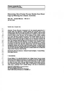
where χi is the opening angle between a particle and the thrust axis vector ~nT , whose direction is defined here to point from the heavy jet mass hemisphere to the light jet mass hemisphere. Although the JCEF is a particularly simple and excellent observable for the determination of αs , it has been rarely used until now in experimental measurements. Within an O(αs2 ) analysis, the region 90◦ < χ ≤ 180◦ , corresponding to the heavy jet mass hemisphere, can be used for the measurement of αs . The distribution of the JCEF is shown in Figure 1. Hadronization corrections and detector corrections as well as the next-to-leading order perturbative corrections are small. This allows a specially wide fit range to be used.

3.2

Fragmentation Models

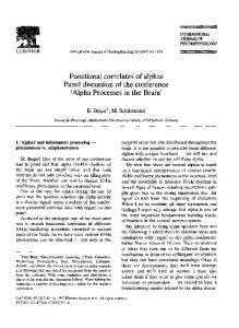
QCD based hadronization models, which describe well the distributions of the event shape observables in the hadronic final state of e+ e− annihilation, are commonly used for modelling the transition from the primary quarks to the hadronic final state. Perturbative QCD can describe only a part of this transition, the radiation of hard gluons and the evolution of a parton shower. For a determination of the strong coupling constant αs one has to take account of the so-called fragmentation or hadronization process, which is characterized by a small momentum transfer and hence a breakdown of perturbation theory. Several Monte Carlo models are in use to estimate the size of the hadronization effects and the corresponding uncertainty. The most frequently used fragmentation models, namely JETSET 7.3 PS [8], ARIADNE 4.06 [20] and HERWIG 5.8c [21] have been extensively studied and tuned to DELPHI data and to identified particle spectra from all LEP experiments in [22]. As discussed in detail in [22] all models describe the data well. Examples of the measured hadron distributions are presented in Figures 1 and 2. The increased systematic accuracy of the data is partially due to the fact that the ϑT dependence of the detector corrections is explicitly taken into account. The ϑT dependence of the detector corrections is shown, for instance, in Figure 2 for two of the observables studied. Detailed tables of the individual event shape distributions including

8

their statistical and systematic errors will be made available in the HEPDATA database [23]. For figures of the distributions see also [24]. Before theoretical expressions describing parton distributions can be compared with experimental data, corrections have to be made for hadronization effects, i.e. effects resulting from the transition of the parton state into the observed hadronic state. For the global event shape observables this transition is performed by a matrix P, where Pij is the probability that an event contributing to the bin j of the partonic distribution will contribute to the bin i in the hadronic distribution and is computed from a Monte Carlo model. This probability matrix has been applied to the distributions from O(αs2 ) perturbative theory Dpert. (Y, cos ϑT ) to obtain the distributions for the predictions of the observed final state Dhadr. (Y, cos ϑT ): X Dhadr. (Y, cos ϑT )i = Pij (Y, cos ϑT )Dpert. (Y, cos ϑT )j . (26) j

In the case of the JCEF, EEC and AEEC, which are defined in terms of single particles and pairs of particles, respectively, bin-by-bin correction factors CHadr. similar to that described above for the detector effects have been computed such as: Dhadr. (Y, cos ϑT )i = CHadr. (Y, cos ϑT )i Dpert. (Y, cos ϑT )i

.

(27)

Our reference model for evaluating hadronization effects is the JETSET 7.3 Parton Shower (PS) Generator, which has been modified with respect to the heavy particle decays to obtain a better description of the heavy particle branching fraction. This modified version is denoted by JETSET 7.3 PS D in the following. The tuned parameters have been taken from [22], where the updated tuning procedure is described in detail. In order to estimate the systematic error of the hadronization correction, the analysis was repeated using alternative Monte Carlo generators with different hadronization models. In addition, the parameters for the JETSET PS were varied. A description of the models and their differences can be found for example in [22]. The alternative models used are ARIADNE 4.06, HERWIG 5.8c as well as version 7.4 JETSET PS [8]. All these models have been tuned to DELPHI data [22]. For our standard Monte Carlo program we applied also an alternative tuning to the DELPHI data which includes Bose-Einstein correlations, not included in the reference tuning. Whereas the number of hard gluons predicted by second order QCD matrix elements is simulated by the hadronization models [25], additional soft gluons are produced within the parton shower cascade, controlled by the JETSET PS parameter Q0 , which describes the parton virtuality at which the parton shower is stopped. To account for the sensitivity of the shape observables with respect to the additional soft gluons, Q0 has been varied from 0.5 GeV to 4.0 GeV. The systematic error of αs originating from hadronization corrections is then estimated as the variance of the fitted αs values obtained by using all the hadronization corrections mentioned above. Further studies have been made to investigate the influence of the main fragmentation parameters of the JETSET PS model by varying them within their experimental uncertainty. It has been found that this contribution to the uncertainty of αs in general is less than one per mille, and has been neglected.

Det.Corr. JCEF(χ) (rad ) Hadr.Corr.

1.5 1.25 1 0.75 0.5

1.2 1 0.8 1.5 1.25 1 0.75 0.5

-1

Det.Corr. 1/σ dσ/d(1-T) Hadr.Corr.

1.2 1 0.8

DELPHI DATA

DELPHI

JETSET 7.3 PS D JETSET 7.4 PS

10 HERWIG 5.8 C

DELPHI DATA

DELPHI

JETSET 7.3 PS D JETSET 7.4 PS ARIADNE 4.06 HERWIG 5.8 C

1

1 10

-1

Fit Range

Fit Range (MC-Data)/Data

(MC-Data)/Data

10

-1

0.1 0.05 0 -0.05 -0.1 0

0.05

0.1

0.15

0.2

0.25

0.3

0.35 1-T

10 0.1 0.05 0 -0.05 -0.1

-2

90

100

110

120

130

140

150

160

170

180

χ (degree)

9

Figure 1: left part: Measured 1-T distribution integrated over cos ϑT . The upper part shows the detector correction including effects due to initial state radiation. The part below shows the size of the hadronization correction. The width of the band indicates the uncertainty of the correction. In the central part the measured 1-T distribution is compared to the expectation from four hadronization generators, JETSET 7.3 PS D with DELPHI modification of heavy particle decays, JETSET 7.4 PS, ARIADNE 4.06 and HERWIG 5.8c. Also shown is the 1-T range used in the QCD fit. The lower part shows the ratio (Monte Carlo simulation-data)/data for the four hadronization generators. The width of the band indicates the size of the experimental errors. right part: Same curves as shown in the left part but for JCEF integrated over cos ϑT .

Det.Corr. JCEF(χ) (rad )∆Hadr.Corr.

0.04 0.02 0 -0.02 -0.04

1.2 1 0.8 0.04 0.02 0 -0.02 -0.04

-1

Det.Corr. 1/σ dσ/d(1-T)∆Hadr.Corr.

1.2 1 0.8

DELPHI DATA

DELPHI

0. ≤ cos ϑT < 0.12 0.72 ≤ cos ϑT < 0.82

10

JETSET 7.3 PS D

DELPHI DATA

DELPHI

0. ≤ cos ϑT < 0.12 0.72 ≤ cos ϑT < 0.82 1

JETSET 7.3 PS D

0. ≤ cos ϑT < 0.12

0. ≤ cos ϑT < 0.12

0.72 ≤ cos ϑT < 0.82

0.72 ≤ cos ϑT < 0.82

1 10

-1

Fit Range

Fit Range (MC-Data)/Data

(MC-Data)/Data

10

-1

0.1 0.05 0 -0.05 -0.1 0

0.05

0.1

0.15

0.2

0.25

0.3

0.35 1-T

10 0.1 0.05 0 -0.05 -0.1

-2

90

100

110

120

130

140

150

160

170

180

χ (degree)

Figure 2: left part: Measured 1-T distribution in two bins of cos ϑT . The upper part shows the detector corrections in the two cos ϑT bins. The part below shows the size of the relative hadronization correction in the two cos ϑT bins with respect to the average correction. In the central part the measured 1-T distributions are compared to JETSET 7.3 PS D. The lower part shows the ratio (Monte Carlo simulation-data)/data for the two cos ϑT bins. right part: Same curves as shown in the left part but for JCEF in two bins of cos ϑT . 10

11

4

Comparison with Angular Dependent Second Order QCD using Experimentally Optimized Scales

The evaluation of the O(αs2 ) coefficients is performed by using EVENT2 [26], a program for the integration of the O(αs2 ) matrix elements. The algorithm is described in [1]. Using this program, one can calculate the double differential cross-section for any infrared and collinear safe observable Y in e+ e− annihilation as a function of the event orientation: 1 d2 σ(Y, cos ϑT ) = α ¯ s (µ2 ) · A(Y, cos ϑT ) σtot dY d cos ϑT     2 2 + α ¯ s (µ ) · B(Y, cos ϑT ) + 2πβ0 ln(xµ ) − 2 A(Y, cos ϑT ) ,(28) where α ¯ s = αs /2π and β0 = (33 − 2nf )/12π, nf is the number of active quark flavours and σtot is the one loop corrected cross-section for the process e+ e− → hadrons. The event orientation enters via ϑT , which denotes the polar angle of the thrust axis with respect to the e+ e− beam direction. The renormalization scale factor xµ is defined by µ2 = xµ Q2 where Q = MZ is the centre-of-mass energy. A and B denote the O(αs ) and O(αs2 ) QCD coefficients, respectively. Alternatively, the double differential cross-section can be normalized to the partial cross-section in each cos ϑT interval:  −1 2 dσ d σ(Y, cos ϑT ) R(Y, cos ϑT ) = (29) d cos ϑT dY d cos ϑT which is more appropriate for the study of residual QCD effects.

The strong coupling αs at the renormalization scale µ is in second order perturbative QCD expressed as ! 2 β1 ln ln Λµ 2 1 1− 2 , (30) αs (µ) = 2 β0 ln µ22 β0 ln µ 2 Λ

Λ

(5)

where Λ ≡ ΛMS is the QCD scale parameter computed in the Modified Minimal Subtraction (MS) scheme for nf = 5 flavours and β1 = (153 − 19nf )/24π 2 . The renormalization scale µ is a formally unphysical parameter and should not enter at all into an exact infinite order calculation [27]. Within the context of a truncated finite order perturbative expansion for any particular process under consideration, the definition of µ depends on the renormalization scheme employed, and its value is in principle completely arbitrary. This renormalization scale problem has been discussed extensively in the literature [4,27,28]. The traditional experimental approach to account for this problem has been to measure all observables at the same fixed scale value, the so-called physical scale xµ = 1 or equivalently µ2 = Q2 . The scale dependence has been taken into account by varying µ over some wide ad hoc range, quoting the resulting change in the QCD predictions as

12

theoretical uncertainty. However, the approach of choosing xµ = 1 has a severe disadvantage. If we consider the ratio of the O(αs ) and the O(αs2 ) contributions to the cross-section, defined as h i αs (xµ ) B(Y ) + A(Y )(2πβ0 ln(xµ ) − 2) , (31) rN LO (Y ) = A(Y ) we find for many observables quite large values for the second order contributions. In some cases this ratio can have a magnitude approaching unity, indicating a poor convergence behavior of the O(αs2 ) predictions in the MS scheme which would quite naturally result in a wide spread of the measured αs values. This has indeed been observed in previous analyses using O(αs2 ) QCD [2,29,30]. Several proposals have been made which resolve the problem by choosing optimized scales according to different theoretical prescriptions [31,32,33]. These methods have been discussed with some controversy [27] and until now no consensus has been achieved. The only approach for determining an optimized scale value, which does not rely on specific theoretical assumptions, is the experimental evaluation of an optimized O(αs2 ) scale value xµ for each measured observable separately. This strategy has therefore been chosen to be the primary method. For previous analyses including experimentally optimized renormalization scales see for example [29,34]. The theoretical approaches for choosing an optimized renormalization scale value are studied in detail in Section 5. As will be shown later, the approach of applying experimentally optimized scales yields an impressive consistency of the αs (MZ2 ) measurements from different observables. The procedure applied here, is a combined fit of αs and the scale parameter xµ . In the past this strategy suffered from a poor sensitivity of the fit with respect to xµ for most of the observables. Due to the high statistics and high precision data now available, one may expect a better sensitivity at least for some of the observables under consideration. We determined αs (MZ2 ) and the renormalization scale factor xµ simultaneously by comparing the corrected distributions for each observable Y with the perturbative QCD calculations corrected for hadronization effects as described in the previous section. The theoretical predictions have been fitted to the measured distributions R(Y, cos ϑT ) by minimizing χ2 , defined by using the sum of the squares of the statistical and systematic experimental errors, with respect to the variation of ΛM S and xµ . The fit range for the central analysis, i.e. including the experimental optimization of xµ , was chosen according to the following considerations: • Requiring a detector acceptance larger than 80%, the last bin in cos ϑT was excluded in general, i.e. the fit range was restricted to the interval 0 ≤ cos ϑT < 0.84 which corresponds to the polar angle interval 32.9◦ < ϑT ≤ 90.0◦ . • Acceptance corrections were required to be below about 25% and the hadronization corrections to be below ∼ 40%. • The contribution of the absolute value of the second order term rN LO (Y ) as defined in Eq. (31) was required to be less than one3 over the whole fit range. 3 This requirement restricts the fit interval only for the total jet broadening observable B sum , which yields rather large O(α2s ) contributions for any choice of the renormalization scale value.

13

• The requirement that the data can be well described by the theoretical prediction, i.e. χ2 /ndf is approximately 1 and stable over the fit range. • Stability of the αs - measurement with respect to the variation of the fit range. For the analysis with a fixed renormalization scale value xµ = 1, the requirement that χ2 /ndf is approximately 1 can in general not be applied, since it would cause an unreasonably large reduction of the fit range for many observables. The thrust distribution for example could be fitted only over a range of at most three bins. For further details see also Section 4.2. The fit ranges for this analysis as well as for the analyses applying theoretically motivated scale setting methods have therefore been chosen identical to the analysis with experimentally optimized scale values, regardless of the χ2 values of the fits.

4.1

Systematic and Statistical Uncertainties

For each observable the uncertainties from the fit of αs (MZ2 ) and of xµ have been determined by changing the parameters corresponding to a unit increase of χ2 . In the case of asymmetric errors the higher value was taken. The systematic experimental uncertainty was estimated by repeating the analysis with different selections to calculate the acceptance corrections as described in Section 2. Additionally, an analysis was performed including neutral clusters measured with the hadronic and/or electromagnetic calorimeters. The overall uncertainty was taken as the variance of the individual αs (MZ2 ) measurements. An additional source of experimental uncertainty arises from the determination of the fit range, which has been estimated by varying the lower and the upper edge of the fit range by ±1 bin, respectively, while the other edge is kept fixed. Half of the maximum deviation in αs (MZ2 ) has been taken as the error due to the variation of the fit range and has been added in quadrature. The hadronization uncertainty was determined as described in Section 3. The total uncertainty on αs (MZ2 ) is determined from the sum of the squares of the errors listed above. Uncertainties due to Missing Higher Order Calculations An additional source of theoretical uncertainty arises due to the missing higher order calculations of perturbative QCD. It is commonly assumed, that the size of these uncertainties can be estimated by varying the renormalization scale value applied for the determination of αs (MZ2 ) within some ‘reasonable’ range [35]. The choice of a ‘reasonable’ range involves subjective jugdement and so far no common agreement about the size of this range has been achieved. Furthermore, this commonly used approach has been criticized in the literature [4]. According to [4] any artificial increase of the uncertainty of αs (MZ2 ) due to a large variation of the renormalization scale should be avoided so that the degree of precision to which QCD can be tested remains transparent. It should be pointed out that no such additional uncertainty is required to understand the scatter of the measurements from a large number of observables if experimentally optimized renormalization scale values are applied. This will be demonstrated in the following section.

14

Other procedures for estimating uncertainties due to missing higher order corrections have been suggested, in particular the comparison of αs (MZ2 ) values obtained by applying different reasonable renormalization schemes or by replacing the missing higher order terms by their Pad´e Approximants [35]. Both strategies have been studied. By comparing the size of the uncertainties derived applying these methods (see e.g. Table 11), a exp variation of xµ between 0.5 · xexp µ and 2 · xµ seems justified to obtain an estimate of these uncertainties. Similar or identical ranges have for example also been chosen in [3,57].

4.2

Results

The results of the fits to the 18 event shape distributions are summarized in tables 1 and 2 and shown in Figure 3. It should be noted that for all observables the normalized χ2 is about one for a typically large number of degrees of freedom (ndf = 16 − 236, see Table 1). The individual errors contributing to the total error on the value of αs are listed in Table 2. Among the observables considered the JCEF yields the most precise result. For comparison, the data have also been fitted in O(αs2 ) applying a fixed renormalization scale value xµ = 1. The results of these fits are summarized in table 3 and shown in Figure 4. As can be seen from the χ2 /ndf values of the fits, the choice of xµ = 1 yields only a poor description of the data for most of the observables, for many observables the

Observable Fit Range cos ϑT Range ◦ ◦ EEC 28.8 − 151.2 0.0 - 0.84 AEEC 25.2◦ − 64.8◦ 0.0 - 0.84 JCEF 104.4◦ − 169.2◦ 0.0 - 0.84 1−T 0.05 - 0.30 0.0 - 0.84 O 0.24 - 0.44 0.0 - 0.84 C 0.24 - 0.72 0.0 - 0.84 BMax 0.10 - 0.24 0.0 - 0.84 BSum 0.12 - 0.24 0.0 - 0.84 ρH 0.03 - 0.14 0.0 - 0.84 ρS 0.10 - 0.30 0.0 - 0.36 ρD 0.05 - 0.30 0.0 - 0.84 E0 D2 0.07 - 0.25 0.0 - 0.84 DP0 0.05 0.18 0.0 - 0.84 2 P D2 0.10 - 0.25 0.0 - 0.84 DJade 0.06 0.25 0.0 - 0.84 2 Durham D2 0.015 - 0.16 0.0 - 0.84 DGeneva 0.015 0.03 0.0 - 0.84 2 Cambridge D2 0.011 - 0.18 0.0 - 0.84

xµ χ2 /ndf 0.0112 ± 0.0006 1.02 0.0066 ± 0.0018 0.98 0.0820 ± 0.0046 1.05 0.0033 ± 0.0002 1.24 2.30 ± 0.40 0.90 0.0068 ± 0.0006 1.02 0.0204 ± 0.0090 0.89 0.0092 ± 0.0022 1.19 0.0036 ± 0.0004 0.63 0.0027 ± 0.0019 0.82 2.21 ± 0.38 1.02 0.048 ± 0.020 0.85 0.112 ± 0.048 1.02 0.0044 ± 0.0004 1.00 0.126 ± 0.049 1.05 0.0126 ± 0.0015 0.92 7.10 ± 0.28 0.84 0.066 ± 0.019 0.98

ndf 236 75 124 89 33 82 47 40 54 16 68 68 68 47 75 96 19 145

Table 1: Observables used in the O(αs2 ) QCD fits. For each of the observables the fit range, the range in cos ϑT , the measured renormalization scale factor xµ together with the uncertainty as determined from the fit, the χ2 /ndf and the number of degrees of freedom ndf are shown. In the case of asymmetric errors the higher value is given.

15

description is even unacceptable. More details concerning the QCD fits are presented in Figures 5 to 9. Figure 5 shows the values of αs (MZ2 ) and the corresponding values of ∆χ2 , i.e. the change of χ2 with respect to the optimal value, for the fits as a function of the scale lg(xµ ) for some of the investigated observables. The shape of the ∆χ2 curves indicates that for most distributions the renormalization scale has to be fixed to a rather narrow range of values in order to be consistent with the data. For most of the observables the renormalization scale dependence of αs (MZ2 ) is significantly smaller in the region of the scale value for the minimum in χ2 /ndf than for the region around xµ = 1. It should however be noted, that even for observables exhibiting a strong scale dependence of αs (MZ2 ) , e.g. D2Geneva , the αs (MZ2 ) value for the experimentally optimized scale value is perfectly consistent with the average value. Figures 6 to 9 contain a direct comparison of the data measured at various bins in cos ϑT with the results of the QCD fits. The measured dependence on both cos ϑT and the studied observable are precisely reproduced by the fits. At this point a comparison with the results from applying a fixed renormalization scale value xµ = 1 seems appropriate. Figure 10 shows QCD fits to the data with experimen-

Observable EEC AEEC JCEF 1−T O C BMax BSum ρH ρS ρD DE0 2 DP0 2 DP2 DJade 2 DDurham 2 DGeneva 2 DCambridge 2

αs (MZ2 ) ∆αs (Exp.) ∆αs (Hadr.) ∆αs (Scale.) 0.1142 ± 0.0007 ± 0.0023 ± 0.0014 0.1150 ± 0.0037 ± 0.0029 ± 0.0100 0.1169 ± 0.0006 ± 0.0013 ± 0.0008 0.1132 ± 0.0009 ± 0.0026 ± 0.0023 0.1171 ± 0.0028 ± 0.0030 ± 0.0038 0.1153 ± 0.0021 ± 0.0023 ± 0.0017 0.1215 ± 0.0022 ± 0.0031 ± 0.0013 0.1138 ± 0.0030 ± 0.0032 ± 0.0030 0.1215 ± 0.0014 ± 0.0029 ± 0.0050 0.1161 ± 0.0014 ± 0.0018 ± 0.0016 0.1172 ± 0.0013 ± 0.0034 ± 0.0007 0.1165 ± 0.0027 ± 0.0029 ± 0.0017 0.1210 ± 0.0018 ± 0.0026 ± 0.0009 0.1187 ± 0.0019 ± 0.0021 ± 0.0036 0.1169 ± 0.0011 ± 0.0020 ± 0.0028 0.1169 ± 0.0013 ± 0.0016 ± 0.0015 0.1178 ± 0.0052 ± 0.0075 ± 0.0295 0.1164 ± 0.0008 ± 0.0023 ± 0.0004

∆αs (Tot.) ± 0.0028 ± 0.0111 ± 0.0017 ± 0.0036 ± 0.0056 ± 0.0036 ± 0.0041 ± 0.0053 ± 0.0060 ± 0.0033 ± 0.0038 ± 0.0044 ± 0.0033 ± 0.0046 ± 0.0040 ± 0.0026 ± 0.0309 ± 0.0025

Table 2: Individual sources of errors of the αs (MZ2 ) measurement. For each observable, the value of αs (MZ2 ) , the experimental uncertainty (statistical and systematic), the uncertainty resulting from hadronization corrections, the theoretical uncertainty due to scale variation around the central value xexp in the range 0.5 · xexp ≤ xµ ≤ 2 · xexp and µ µ µ the total uncertainty are shown.

16

tally optimized and with fixed renormalization scale values xµ = 1 for the observables 1 − T , ρH and D2P . It can be seen that the slope of the experimental distributions cannot be described by the theoretical prediction applying xµ = 1. The same observation has also been made for other observables. Good description of the data can in general only be achieved within the small kinematical region where the fit curve intersects with the data. Demanding χ2 /ndf ⋍ 1 the thrust distribution for example can only be described within a maximum range of three bins in 1-T. It should be noted, that in contrast to fits applying experimentally optimized scales, the stability of αs (MZ2 ) with respect to the choice of the fit range is in general quite poor. This observation is new and due to the fact that the data used in this analysis have both smaller statistical and systematical errors than in previous publications. (See also Section 4.3) and [39]. Combining the 18 individual results from the αs (MZ2 ) measurements applying experimentally optimized renormalization scale values by using an unweighted average yields αs (MZ2 ) = 0.1170 ± 0.0025 whereas the corresponding average for the measurements using the fixed scales xµ = 1 is αs (MZ2 ) = 0.1234 ± 0.0154. For the experimentally optimized scales the scatter of the individual measurements is significantly reduced. The consistency of the individual measurements using experimentally optimized scales is clearly shown by the good χ2 /ndf = 9.6/17 for the unweighted average. This value is

Observable EEC AEEC JCEF 1−T O C BMax BSum ρH ρS ρD DE0 2 DP0 2 DP2 DJade 2 DDurham 2 DGeneva 2 DCambridge 2

αs (MZ2 ) ∆αs (Scale) 0.1297 ± 0.0037 0.1088 ± 0.0015 0.1191 ± 0.0012 0.1334 ± 0.0042 0.1211 ± 0.0065 0.1352 ± 0.0043 0.1311 ± 0.0073 0.1403 ± 0.0056 0.1325 ± 0.0036 0.1441 ± 0.0055 0.1181 ± 0.0012 0.1267 ± 0.0033 0.1265 ± 0.0026 0.1154 ± 0.0019 0.1249 ± 0.0030 0.1222 ± 0.0034 0.0735 ± 0.0071 0.1202 ± 0.0021

∆αs (Tot.) χ2 /ndf ± 0.0042 10.7 ± 0.0050 2.04 ± 0.0024 7.7 ± 0.0051 25.9 ± 0.0077 2.38 ± 0.0053 12.0 ± 0.0083 1.67 ± 0.0071 8.1 ± 0.0049 5.1 ± 0.0062 2.16 ± 0.0039 1.54 ± 0.0052 1.35 ± 0.0041 1.31 ± 0.0036 5.35 ± 0.0042 1.53 ± 0.0046 3.47 ± 0.0116 120. ± 0.0033 1.32

Table 3: Results of the αs (MZ2 ) measurements using a fixed renormalization scale xµ = 1. For each observable, the value of αs (MZ2 ) , the uncertainty from the variation of the scale between 0.5 ≤ xµ ≤ 2, the total uncertainty and the χ2 /ndf of the fit are shown.

17

computed on the basis of the total uncertainty (experimental and hadronization uncertainty) without considering an additional renormalization scale error. For the average of the fixed scale xµ = 1 measurements χ2 /ndf = 168/17, thus in this case the individual measurements are clearly inconsistent with each other. This inconsistency may be understood to arise from the imperfect description of the data for the fits with xµ = 1, which cause αs , the parameter of the fit, not to be well defined. The idea behind the common analysis of such a large number of observables is to optimize the use of the information contained in the complex structure of multi-hadron events. Errors due to the corrections for hadronization effects may be expected to cancel to some extent in the averaging procedure. To test this expectation the analysis of each of the individual 18 observables is repeated by performing hadronization corrections with all hadronization generators described in Section 3.2. This results in 7 times 18 individual αs values. As a first test for each of the 18 observables the unweighted average value of αs from the seven models is evaluated. The average value of the 18 αs values is αs (MZ2 ) = 0.1177 ± 0.0029. In a second step for each of the 7 hadronization models an unweighted average of the corresponding 18 αs values is calculated. Finally an unweighted average of the 7 average values for the different hadronization models is computed resulting in αs (MZ2 ) = 0.1177 ± 0.0016. The result confirms that the scatter of the average values due to different assumptions for hadronization corrections is significantly smaller than the uncertainty of ±0.0025 of the mean value from 18 individual observables. The correlations between the αs values obtained from the different observables must be taken into account in order to calculate their weighted average. Since the correlations are mostly unknown, the exact correlation pattern cannot be worked out reliably. Therefore, we use a recently proposed method [36], which makes use of a robust estimation of the covariance matrix and has been used for example in [37]. Here it is assumed that different measurements i and j are correlated with a fixed fraction ρeff of the maximum possible correlation Cmax ij : Cij = ρeff Cijmax

i 6= j,

with Cijmax = σi σj

.

(32)

For ρeff = 0 the measurements are treated as uncorrelated, for ρeff = 1 as 100% correlated entities. When χ2 < ndf the measurements are assumed to be correlated and the value ρeff then is adjusted such that the χ2 is equal to the number of degrees of freedom ndf : X χ2 (ρeff ) = (xi − x)(xj − x)(C −1 )ij = n − 1 = ndf . (33) i,j

When χ2 > ndf it is assumed that the errors of the measurement are underestimated and will therefore be scaled until χ2 = ndf is satisfied.

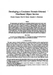
Applying this method to the 18 observables studied, the weighted average (see also Fig. 3) yields: αs (MZ2 ) = 0.1168 ± 0.0026 with ρeff being 0.635. Both the central value and its uncertainty are almost identical to the unweighted average and the r.m.s. quoted above, which in itself is a remarkable result.

18

It should be noted, that the method applied for the calculation of the weighted average does not necessarily lead to the smallest possible error. In [37] it is shown for example, that the error of the weighted average is increased if less significant measurements are included. Within this analysis however, the αs measurements from all individual observables have been considered, regardless of their significance. This is motivated by the fact that the errors of the αs measurements quoted in Table 2 and in the following subsections contain all uncertainties which can be evaluated from a careful experimental analysis. However, the spread of the αs measurements may not be explainable by the individual uncertainties alone, there may be additional uncertainties, which cannot be derived from a single observable. Therefore the above averaging procedure has been applied and robustness of the error estimate has been preferred instead of minimizing the error. Still this error estimate may not cover a possible general shift of the measured average with respect to the true αs (MZ2 ) value. Apart from a better theoretical understanding, today such a shift could only be inferred by comparing to different types of calculation, like resummed or Pad´e approximation, which are presented in Sections 6 and 7.

4.3

Additional Cross Checks

An underlying assumption for the O(αs2 ) QCD fits to the shape observables is that the value of αs is approximately independent of a variation of the renormalization scale within the fit range. To check this assumption, a cross check for the differential two jet rate observables has been performed following a suggestion in [38]. For these observables the QCD fits have been repeated, allowing the renormalization scale to vary proportion√ 2 ally to ycut , i.e. µ = xµ ycut s. The differences in the αs (MZ2 ) determination have been found to be of the order of a few per mille for the individual jet rate observables and to be less than two per mille for the average of these observables. A further investigation has been performed for all observables of Table 1. The fit range listed in Table 1 has been divided into two separate, approximately symmetrical regions, allowing a maximum overlap of one bin. αs (MZ2 ) has been determined applying experimentally optimized scales for both regions independently. The fits were successful for all observables except D2Geneva , where the resulting fit ranges were too small to allow the fits to converge. Good agreement of the two αs values measured for each observable is found. In a further step, the two αs (MZ2 ) values have been combined for each observable according to their statistical weight. These αs values have been combined by calculating a weighted average as described before. The resulting average value of αs (MZ2 ) = 0.1168 ± 0.0025 is identical to the value determined from the standard procedure. No systematical trend of the two values of the renormalization scales found for the two fit ranges (dominated by two respectively three jet events) is observed. Further information on this study can be found in [39].

19

DELPHI

EEC AEEC JCEF 1-Thr O C BMax BSum ρH ρS ρD D2E0 D2P0 D2P D2Jade D2Durham D2Geneva D2Cambridge w. average :

0.06

0.08

0.1

xµ exp. opt.

αS(MZ2) = 0.1168 ± 0.0026 2 χ /ndf = 6.2 / 17 ρeff = 0.635

0.12

0.14

0.16

0.18

αS (MZ2) Figure 3: Results of the QCD fits applying experimentally optimized scales for 18 event shape distributions. The error bars indicated by the solid lines are the quadratic sum of the experimental and the hadronization uncertainty. The error bars indicated by the dotted lines include also the additional uncertainty due to the variation of the renormalization scale due to scale variation around the central value xexp in the range µ exp exp 0.5 · xµ ≤ xµ ≤ 2 · xµ . Also shown is the correlated weighted average (see text). The χ2 -value is given before readjusting according to Eq. 33.

20

DELPHI

EEC AEEC JCEF 1-Thr O C BMax BSum ρH ρS ρD D2E0 D2P0 D2P D2Jade D2Durham

xµ = 1

D2Geneva D2Cambridge w. average :

0.06

0.08

0.1

αS(MZ2) = 0.1232 ± 0.0116 2 χ /ndf = 71 / 17 ρeff = 0.635 ferr = 3.38

0.12

0.14

0.16

0.18

αS (MZ2) Figure 4: Results of the QCD fits applying a fixed renormalization scale xµ = 1 . The error bars indicated by the solid lines are the quadratic sum of the experimental and the hadronization uncertainty. The error bars indicated by the dotted lines include also the additional uncertainty due to the variation of the renormalization scale around the central value xexp from 0.5 · xexp ≤ xµ ≤ 2 · xexp µ µ µ . Also shown is the correlated weighted average. It has been calculated assuming the same effective correlation ρeff = 0.635 as for the fit results applying experimentally optimized scales. The χ2 /ndf for the weighted average is 71/17, where the χ2 given corresponds to the value before adjusting ρeff . In order to yield χ2 /ndf = 1, the errors have to be scaled by a factor ferr = 3.38.

αs (MZ2 )

αs (MZ2 )

0.15

1-T C O

0.14

EEC JCEF ρD

0.15

D2Durham D2Cambridge D2Geneva

0.14

0.13

0.13

0.12

0.12

0.11

D2Jade D2P D2E0

0.11

DELPHI 2

∆χ

∆χ

2

DELPHI

40

40

20

20

0

-3

-2.5

-2

-1.5

-1

-0.5

0

0.5

1

1.5 lg(xµ )

0

-3

-2.5

-2

-1.5

-1

-0.5

0

0.5

1

1.5 lg(xµ )

21

Figure 5: (left side) αs (MZ2 ) and ∆χ2 = χ2 − χ2min from O(αs2 ) fits to the double differential distributions in cos ϑT and 1 − T, C, O, EEC, JCEF, ρD . Additionally, the χ2 minima are indicated in the αs (MZ2 ) curves. (right side) The same for the double differential distributions in cos ϑT and the differential 2-jet rate applying the Durham, Cambridge, Geneva, Jade, P and E0 jet algorithm.

DELPHI

DELPHI

Figure 6: (left side) QCD fits to the measured thrust distribution for two bins in cos ϑT . (right side) Measured thrust distribution at various fixed values of 1 − T as a function of cos ϑT . The solid lines represent the QCD fit. 22

DELPHI

DELPHI

Figure 7: Same as Figure 6 but for the jet cone energy fraction JCEF

23

DELPHI

DELPHI

Figure 8: Same as Figure 6 but for the energy energy correlation EEC.

24

DELPHI

DELPHI

Figure 9: Same as Figure 6 but for the differential two jet rate with the Jade Algorithm DJade . 2

25

DELPHI DATA O(αs2)

- exp. opt.

O(αs2) - xµ = 1

D2P

1/σ dσ/dρH

1/σ dσ/d(1-T)

10

2

20

DELPHI DATA O(αs2)

DELPHI DATA

- exp. opt.

O(αs2) - xµ = 1

10 9

O(αs2) - exp. opt.

1 0.9 0.8

O(αs2) - xµ = 1

0.7 0.6

8 0.5

7

0.4

6 5

0.3

1 4 0.2 3

2

DELPHI

0.1 0.09 0.08

DELPHI

DELPHI

0.07

Fit Range 10

Fit Range

-1

0

0.05

0.1

0.15

0.2

0.25

0.3

0.35

1-T

1

0.02

0.04

0.06

0.08

Fit Range

0.06 0.1

0.12

0.14

0.16

ρH

0.05

0.1

0.15

0.2

0.25

0.3

ycut

Figure 10: Comparison between O(αs2 ) QCD fits with xµ = 1 and experimentally optimized renormalization scales for the observables 1 − T , ρH and D2P . DELPHI data and theoretical predictions are shown averaged over cos ϑT . The full (dotted) line correspond to fits with experimentally optimized renormalization scale values xexp (xµ = 1), respectively. The theoretical prediction is averaged over the µ bin width and drawn through the bin center.

26

27

5

Scale Setting Methods from Theory

Several methods for the choice of an optimized value for the renormalization scale have been suggested by theory. See e.g. [28] for an overview. In this section we compare the αs (MZ2 ) measurements, using renormalization scales predicted by three different approaches with the αs (MZ2 ) measurements using experimentally optimized scales: (i) The principle of minimal sensitivity (PMS) : Since all order predictions should be independent of the renormalization scale, Stevenson [31] suggests choosing the scale to be least sensitive with respect to its variation, i.e. from the solution of ∂σ =0 . ∂xµ

(34)

(ii) The method of effective charges (ECH) : The basic idea of this approach [32] is to choose the renormalization scheme in such a way that the relation between the physical quantity and the coupling is the simplest possible one. In O(αs2 ) , where the ECH approach is equivalent to the method of fastest apparent convergence (FAC) [32] the scale is chosen in such a way that the second order term in Eq. (28) vanishes: B(Y, cos ϑT ) + (2πβ0 ln(xµ ) − 2)A(Y, cos ϑT ) = 0 .

(35)

(iii) The method of Brodsky, Lepage and MacKenzie (BLM) [33]: This method follows basic ideas in QED, where the renormalized electric charge is fully given by the vacuum polarization due to charged fermion-antifermion pairs [28]. In QCD it is suggested to fix the scale with the requirement that all the effects of quark pairs be absorbed in the definition of the renormalized coupling itself. In O(αs2 ) this amounts to the requirement that xµ is chosen in such a way that the flavour dependence nf of the second order term in Eq. 28 is removed:   ∂ B(Y, nf ) + (2πβ0 ln(xµ ) − 2)A(Y ) =0 . (36) ∂nf nf =5 The results of the αs (MZ2 ) measurements for the individual observables applying the different scale setting prescriptions are listed in table 4. The weighted averages for the different methods yield: (i) PMS method : αs (M2Z ) = 0.1154 ± 0.0045

(χ2 /ndf = 19/17)

(ii) ECH method : αs (M2Z ) = 0.1155 ± 0.0044

(χ2 /ndf = 19/17)

(iii) BLM method : αs (M2Z ) = 0.1174 ± 0.0068

(χ2 /ndf = 29/13)

to be compared with αs (M2Z ) = 0.1168 ± 0.0026 ( χ2 /ndf = 6.2/17) using the experimentally optimized scales.

28

The weighted averages for the different theoretical methods are in agreement with the average using experimentally optimized scales. The scatter of the individual measurements is lowest for the experimentally optimized scales and highest for the BLM method. Whereas for the experimentally optimized scales the fit values for the individual αs (MZ2 ) measurements are perfectly consistent, the consistency for the ECH and the PMS methods is only moderate. The results for the ECH and the PMS methods are very similar, the correlation ρ between ECH and PMS scales is almost 1. In the case of the BLM method the χ2 /ndf indicates that the individual αs (MZ2 ) measurements are inconsistent. Moreover, the fits using the scales predicted by the BLM method did not converge at all for the observables JCEF , O, ρD and D2Geneva . Figure 11 shows the correlation between the logarithms of the experimentally optimized scales and the logarithms of the scales predicted by the ECH, PMS and the BLM methods. For the ECH and the PMS method there are significant correlations of ρ = 0.75 ± 0.11. In the case of BLM there is a slightly negative correlation of ρ = −0.34 ± 0.25, compatible with zero within 1.5 σ. Our results indicate that the ECH and the PMS methods are useful in the case where an experimental optimization can not be performed, whereas the BLM method does not seem to be suitable for the determination of αs (MZ2 ).

29

Observable αsEXP (MZ2 ) αsP M S (MZ2 ) αsECH (MZ2 ) αsBLM (MZ2 ) EEC 0.1142 0.1133 0.1135 0.1142 AEEC 0.1150 0.1063 0.1064 0.1179 JCEF 0.1169 0.1168 0.1169 1−T 0.1132 0.1101 0.1111 0.1133 O 0.1171 0.1128 0.1124 C 0.1153 0.1119 0.1124 0.1144 BMax 0.1215 0.1222 0.1217 0.1268 BSum 0.1138 0.1023 0.1021 0.1118 ρH 0.1215 0.1197 0.1198 0.1258 ρS 0.1161 0.1154 0.1149 0.1169 ρD 0.1172 0.1190 0.1203 DE0 0.1165 0.1145 0.1142 0.1143 2 DP0 0.1210 0.1204 0.1202 0.1232 2 P D2 0.1187 0.1110 0.1108 0.1118 DJade 0.1169 0.1137 0.1134 0.1137 2 Durham D2 0.1169 0.1162 0.1159 0.1241 DGeneva 0.1178 0.1064 0.1171 2 DCambridge 0.1164 0.1164 0.1163 0.1124 2 w. average 0.1168 ± 0.0026 0.1154 ± 0.0045 0.1155 ± 0.0044 0.1174 ± 0.0068 χ2 /ndf 6.2 / 17 19 / 17 19 / 17 29 / 13 Table 4: Comparison of the αs (MZ2 ) values obtained using the different methods for evaluating the renormalization scale suggested by theory. For each observable the αs (MZ2 ) values using experimentally optimized scales and αs (MZ2 ) values for the scales predicted by the PMS, ECH and BLM methods are shown. The errors for the αs (MZ2 ) measurements are assumed to be identical for all methods (see table 2). The weighted averages are calculated using ρeff = 0.635 and scaling the errors to yield χ2 /ndf = 1 in the case of the PMS, ECH and the BLM methods (see text). The χ2 given for the averaging correspond to the values before adjusting ρeff and rescaling the measurement uncertainties. The fits using the scales predicted by BLM did not converge for the observables JCEF, O, ρD and D2Geneva .

DELPHI

1

lg (xµEXP)

lg (xµEXP)

lg (xµEXP)

2

2

DELPHI

1

2

0

0

0

-1

-1

-1

-2

-2

-2

-3

-3

-3

EXP vs. PMS ρ = 0.75 ± 0.11

-4

-5

-5

-4

-3

-2

-1

0

1

lg (xµ

EXP vs. ECH ρ = 0.75 ± 0.11

-4

2 PMS)

-5

-5

-4

-3

-2

-1

0

1

lg (xµ

DELPHI

1

EXP vs. BLM ρ = -0.34 ± 0.25

-4

2 ECH)

-5

-5

-4

-3

-2

-1

0

1

2

lg (xµBLM)

Figure 11: Comparison between the logarithms of the experimentally optimized renormalization scales and the logarithms of scales predicted by PMS, ECH and the BLM method. The vertical error bars indicated represent the uncertainties from the 2-parameter fits in xµ and αs . The vertical bars represent the range of renormalization scale values for the theoretically motivated scale setting methods evaluated from the individual bins within the fit range of each distribution, whereas the central value has been derived by considering the full theoretical prediction within the fit range.

30

31

6

Pad´ e Approximation

An approach for estimating higher-order contributions to a perturbative QCD series is based on Pad´e Approximations. The Pad´e Approximant [N/M] to the series S = S0 + S1 x + S2 x2 + . . . + Sn xn

(37)

is defined [40] by a0 + a1 x + a2 x2 + . . . + aN xN [N/M] ≡ 1 + b1 x + b2 x2 + . . . + bM xM

;

N +M =n

(38)

and [N/M] = S + O(xN +M +1 ) .

(39)

The set of equations (39) can be solved, and by consideration of the terms of O(xN +M +1 ) one can obtain an estimate of the next order term SN +M +1 of the original series. This is called the PA method. Furthermore, for an asymptotic series [N/M] can be taken as an estimate of the sum (PS) of the series to all orders. The PA method has been used successfully to estimate coefficients in statistical physics [40], and various quantum field theories including QCD [41]. Justifications for some of these successes have been found in mathematical theorems on the convergence and renormalization scale invariance of PAs [41]. In many cases the PAs yield predictions for the higher order coefficients in perturbative series with high accuracy, whereas this accuracy is not expected for the lower order predictions such as O(αs3 ) . For the application of the αs (MZ2 ) determination from event shapes, the Pad´e Approximation can serve as a reasonable estimate of the errors due to higher order corrections [42]. For each bin of our observables an estimate for the O(αs3 ) coefficient C(y) can be derived from [0/1] with a0 = A, b1 = −B/A: C P ad´e (y) =

B 2 (y) . A(y)

(40)

It should be noted that the PA predictions C P ad´e (y) are positive by construction which will result in large errors for kinematical regions where the O(αs3 ) contribution is negative. The fit range has therefore been determined in the following way: Starting from the same fit range as in O(αs2 ) , the fit has been accepted if χ2 /ndf ≤ 5. Otherwise the fit range was reduced bin by bin until the fit yielded χ2 /ndf ≤ 5. In addition to the O(αs3 ) fits in the Pad´e Approximation, the PS method has been used as an estimate of the sum of the perturbative series and αs (MZ2 ) has been extracted by fitting the [0/1] approximation directly to the data. Here, the fit range has been chosen to be the same as for the fits in the O(αs3 ) Pad´e approximation. The χ2 dependence of the αs (MZ2 ) fits applying the Pad´e Approximation as a function of the renormalization scale value xµ is quite small, especially for the PS method. For most of the observables αs (MZ2 ) and xµ could not be determined in a simultaneous fit. Therefore, the fits have been done choosing a fixed renormalization scale value xµ = 1. The uncertainty due to

32

the scale dependence of αs (MZ2 ) has been estimated by varying xµ between 0.5 and 2. The fit results for the individual observables are listed in tables 5 and 6. The fit applying PS to the BSum distribution did not converge for any fit range chosen. For the D2Geneva distribution, the fits did not converge for either method. Comparing the fit results of the O(αs3 ) fits in Pad´e Approximation with the fit results in O(αs2 ) applying xµ = 1, as given in table 3 , the scale dependence of αs (MZ2 ) is reduced for most of the observables, as one would expect from measurements using exact calculations in O(αs3 ) . For the PS method, the reduction of the scale dependence is even larger. Here, αs (MZ2 ) is less scale dependent than in the O(αs2 ) fits for all observables considered. Figure 12 shows the scale dependence of αs (MZ2 ) applying the different QCD predictions to the distribution of the Jet Cone Energy Fraction as an example. There is almost no χ2 dependence of the αs (MZ2 ) fits as a function of the renormalization scale for the PS prediction. For the fits applying O(αs3 ) in the Pad´e Approximation, the χ2 dependence is less than for the O(αs2 ) prediction. However, the JCEF is one of the few observables, where a simultaneous fit of αs (MZ2 ) and xµ is possible.

Observable Fit Range αs (MZ2 ) ∆αs (Scale.) ∆αs (Tot.) ◦ ◦ EEC 28.8 − 151.2 0.1189 ±0.0016 ±0.0026 AEEC 25.2◦ − 64.8◦ 0.1074 ±0.0030 ±0.0056 JCEF 104.4◦ − 169.2◦ 0.1169 ±0.0006 ±0.0016 1−T 0.07 - 0.30 0.1207 ±0.0023 ±0.0036 O 0.24 - 0.32 0.1098 ±0.0014 ±0.0044 C 0.32 - 0.72 0.1208 ±0.0023 ±0.0039 BMax 0.10 - 0.24 0.1183 ±0.0016 ±0.0042 BSum 0.14 - 0.18 0.1127 ±0.0016 ±0.0068 ρH 0.03 - 0.14 0.1230 ±0.0015 ±0.0036 ρS 0.10 - 0.30 0.1252 ±0.0024 ±0.0038 ρD 0.07 - 0.30 0.1045 ±0.0015 ±0.0040 DE0 0.05 0.18 0.1159 ±0.0014 ±0.0042 2 DP0 0.05 - 0.18 0.1199 ±0.0011 ±0.0034 2 0.10 - 0.20 0.1128 ±0.0008 ±0.0030 DP2 DJade 0.06 - 0.25 0.1142 ±0.0014 ±0.0032 2 DDurham 0.015 0.16 0.1170 ±0.0009 ±0.0023 2 DCambridge 0.011 - 0.18 0.1164 ±0.0007 ±0.0026 2 2 average 0.1168 ± 0.0054 χ /ndf = 30 / 16 Table 5: Results on αs (MZ2 ) for QCD-Fits including the O(αs3 ) Term in the Pad´e Approximation (PA). For each of the observables the fit range, αs (MZ2 ) , the uncertainty due to scale variation between 0.5 ≤ xµ ≤ 2 and the total uncertainty are shown. The experimental errors and the uncertainties due to the hadronization corrections are assumed to be the same as for the O(αs2 ) measurements. The weighted average is calculated using ρeff = 0.635 and scaling the errors to yield χ2 /ndf = 1 (see text). The χ2 given for the averaging corresponds to the value before adjusting ρeff and rescaling the measurement uncertainties. The fit for D2Geneva did not converge.

33

Assuming the same correlation as in the O(αs2 ) fits, the weighted averages of αs (MZ2 ) over the observables used have been calculated as: αs (M2Z ) = 0.1168 ± 0.0054 for the PA fits and αs (M2Z ) = 0.1157 ± 0.0037 for the PS fits. The averages are in excellent agreement with the O(αs2 ) value of αs (M2Z ) = 0.1168 ± 0.0026 using optimized scales. The scatter between the observables, however, is somewhat larger than in the O(αs2 ) case. The χ2 /ndf for the average values is 30/16 and 17/15 respectively.

Observable αs (MZ2 ) ∆αs (Scale.) ∆αs (Tot.) EEC 0.1147 ±0.0003 ±0.0021 AEEC 0.1070 ±0.0002 ±0.0048 JCEF 0.1169 ±0.0003 ±0.0015 1−T 0.1165 ±0.0003 ±0.0028 O 0.1135 ±0.0003 ±0.0042 C 0.1150 ±0.0003 ±0.0032 BMax 0.1196 ±0.0003 ±0.0039 ρH 0.1219 ±0.0004 ±0.0033 ρS 0.1161 ±0.0003 ±0.0029 ρD 0.1098 ±0.0003 ±0.0037 DE0 0.1136 ±0.0003 ±0.0040 2 DP0 0.1198 ±0.0003 ±0.0032 2 P D2 0.1124 ±0.0003 ±0.0029 Jade D2 0.1123 ±0.0003 ±0.0029 DDurham 0.1164 ±0.0003 ±0.0021 2 DCambridge 0.1162 ±0.0003 ±0.0025 2 average 0.1157 ± 0.0037 χ2 /ndf = 17 / 15 Table 6: Results on αs (MZ2 ) for QCD-Fits applying the Pad´e Sum Approximation (PS). For each of the observables αs (MZ2 ) , the uncertainty due to scale variation between 0.5 ≤ xµ ≤ 2 and the total uncertainty are shown. The experimental errors and the uncertainties due to the hadronization corrections are assumed to be the same as for the O(αs2 ) measurements. The weighted average is calculated using ρeff = 0.635 and scaling the errors to yield χ2 /ndf = 1 (see text). The χ2 given for the averaging corresponds to the value before adjusting ρeff and rescaling the measurement uncertainties. The fits for BSum and D2Geneva did not converge.

αs (MZ2 )

34

0.13

JCEF O(αs2) Pade Approx. O(αs3) Pade Sum

0.125

0.12

0.115

∆χ

2

DELPHI

40

20

0 -2

-1.5

-1

-0.5

0

0.5

1 lg(xµ )

Figure 12: αs (MZ2 ) and ∆χ2 = χ2 − χ2min for the distribution of the Jet Cone Energy Fraction as a function of xµ from QCD fits applying O(αs2 ) prediction, O(αs3 ) in Pad´e Approximation and the Pad´e Sum Approximation. Additionally, the χ2 minimum for the O(αs2 ) fit and the renormalization scale value xµ = 1 have been indicated in the αs (MZ2 ) curves.

35

7

QCD in the Next-to-Leading Log Approximation

All orders resummed QCD calculations in the Next-to-Leading Log Approximation (NLLA) matched with O(αs2 ) calculations have been used widely to measure αs (MZ2 ) from event shape observables [3,30]. For a generic event shape observable Y for which the theoretical prediction can be exponentiated, the cumulative cross-section at the scale Q2 ≡ s is defined by: 1 R(Y, αs ) = σ

ZY

dσ dY ′ dY ′

(41)

0

and can be expanded in the form R(Y, αs ) = C(αs ) exp Σ(αs , L) + F (αs , Y ) ,

(42)

where L ≡ ln(1/Y ) and C(αs ) = 1 +

∞ X

Ci α ¯ si

(43)

i=1

Σ(αs , L) =

∞ X

α ¯ si

i=1

F (αs , Y ) =

∞ X

i+1 X

Gij Lm

(44)

j=1

Fi (Y )α ¯ si .

(45)

i=1

The Ci are constant and the Fi (Y ) vanish in the infrared limit Y → 0. The factor Σ to be exponentiated can be written Σ(αs , L) = LfLL (αs L) + fN LL (αs L) + subleading terms ,

(46)

where fLL and fN LL represent the leading and the next-to-leading logarithms. They have been calculated for a number of observables, including 1 − T [43], C [44], Bmax [45], Bsum [45], ρH [46] and D2Durham [47], where the NLLA predictions for Bmax and Bsum entering into this analysis are the recently improved calculations by Yu. L. Dokshitzer et al. [48]. Pure NLLA calculations can be used to measure αs (MZ2 ) in a limited kinematic region close to the infrared limit, where L becomes large. In order to achieve a prediction where the kinematical range can be extended towards the 3 jet region, several procedures have been suggested [49] to match the NLLA calculations with the calculations in O(αs2 ) . The O(αs2 ) QCD formula can be written in the integrated form: RO(α2 ) (Y, αs ) = 1 + A(Y )α ¯ s + B(Y )α ¯ s2 , (47) s where A (Y ) and B (Y ) are the cumulative forms of A(Y, cos ϑT ) and B(Y, cos ϑT ) in Eq. (28), integrated over ϑT . Together with the first and second order part of Eq. (44) g1 (L) = G12 L2 + G11 L

(48)

36

g2 (L) = G23 L3 + G22 L2 + G21 L ,

(49)

the ln R matching scheme can be defined as: ln R(Y, αs ) = Σ(αs , L) + H1 (Y )α ¯ s + H2 (Y )α ¯ s2 ,

(50)

H1 (Y ) = A(Y ) − g1 (L)

(51)

where

1 (52) H2 (Y ) = B(Y ) − A2 (Y ) − g2 (L). 2 When combining O(αs2 ) predictions with NLLA calculations one has to take into account that the resummed terms do not vanish at the upper kinematic limit Ymax of the event shape distributions. In order to correct for this, the resummed logarithms are redefined [50] by: L = ln(1/Y − 1/Ymax + 1).

(53)

Several other matching schemes can be defined which differ in the treatment of the subleading terms, thus introducing a principal ambiguity in the matching procedure. The ln R matching scheme has become the preferred one, because it includes the C2 and the G21 coefficients implicitly and uses only those NLLA terms which are known analytically. It yields the best description of the data in terms of χ2 /ndf in most cases [3]. Therefore, we quote the results for the matched predictions using the ln R matching scheme and use the R and R − G21 matching schemes as defined e.g. in [3] for the estimation of the uncertainty due to the matching ambiguity.

7.1

Measurement of αs (MZ2 ) using pure NLLA predictions

To measure αs (MZ2 ) from pure NLLA calculations the fit range has to be restricted to the extreme 2-jet region, where L becomes large and the resummed logarithms dominate. We define ω as the ratio of the resummed logarithms to the non-exponentiating second order contributions as follows : ω=

Σ(αs , L) H1 (Y )α ¯ s + H2 (Y )α ¯ s2

(54)

In addition to the fit range criteria listed in Section 4 we require the minimum of the ratio ω over the fit range not to fall below 5 for the fits in pure NLLA. This leads to the fit ranges listed in table 7. For the observable D2Durham the ratio ω remains small even for small values of ycut . No fit range can be found where the resummed logarithms dominate the prediction. Therefore D2Durham has not been used for the fits in pure NLLA. Contrary to the O(αs2 ) predictions an optimization of the renormalization scale (or more precisely an optimization of the renormalization scheme) cannot be easily performed for the resummed NLLA predictions [4]. Therefore the scale was fixed to xµ = 1. The uncertainty due to the scale dependence of αs (MZ2 ) was estimated by varying the scale xµ between 0.5 and 2.

37

Observable Fit Range (NLLA) Fit Range (matched) 1−T 0.04 - 0.09 0.04 - 0.30 C 0.08 - 0.16 0.08 - 0.72 Bmax 0.02 - 0.04 0.02 - 0.24 Bsum 0.06 - 0.08 0.06 - 0.24 ρH 0.03 - 0.06 0.03 - 0.30 DDurham 0.015 - 0.16 2 Table 7: Fit range for the observables in pure NLLA and matched NLLA fits. The observable D2Durham has not been used for pure NLLA fits, since no fit range can be found, where the resummed logarithms dominate the predictions (see text). The fit results for the individual observables are listed in table 8. The weighted average of αs (MZ2 ) for the 5 observables is αs (MZ2 ) = 0.116 ± 0.006 which is in excellent agreement with the average value for the O(αs2 ) fits of αs (MZ2 ) = 0.1168 ± 0.0026.

Observable αs (MZ2 ) ∆αs (exp.) ∆αs (had.) ∆αs (scal.) ∆αs (tot.) χ2 /ndf 1−T 0.120 ±0.001 ±0.004 ±0.004 ±0.006 0.59 C 0.116 ±0.002 ±0.003 ±0.004 ±0.006 0.53 Bmax 0.111 ±0.004 ±0.003 ±0.002 ±0.006 2.37 Bsum 0.116 ±0.003 ±0.004 ±0.002 ±0.006 1.24 ρH 0.117 ±0.004 ±0.006 ±0.004 ±0.009 0.43 average 0.116 ± 0.006 χ2 /ndf = 1.2 / 4 ρeff = 0.71 Table 8: Results for the αs (MZ2 ) fits in pure NLLA for the individual observables together with the individual sources of uncertainties and the χ2 /ndf for the NLLA fits. The total error on αs (MZ2 ) listed, is the quadratic sum of the experimental error (statistical and systematic uncertainty), the uncertainty due to the hadronization correction and the uncertainty due to the scale dependence of αs (MZ2 ) . Also listed is the weighted average of αs (MZ2 ) for the 5 observables together with the χ2 /ndf for the averaging procedure and the correlation parameter ρeff . The χ2 corresponds to the value before readjusting according to Eq. 33.

38

7.2

Measurement of αs (MZ2 ) using NLLA predictions matched with O(αs2 )

For the QCD fits using NLLA theory matched with O(αs2 ) predictions the fit range has been chosen as the combined fit range for the pure NLLA and the O(αs2 ) fits. The results for the individual observables in the ln R matching scheme are listed in table 9. The additional uncertainty due to the matching ambiguity has been estimated as the maximum difference of αs (MZ2 ) in the ln R matching scheme and the two alternative matching schemes, R and R − G21 . The dependence on the choice of Ymax , i.e. the value of the upper kinematic limit for the shape observables used for the redefinition of the resummed logarithms according to Eq. 53, has been studied by repeating the fits with the value of Ymax being reduced by 10 %. The resulting variation in αs (MZ2 ) has been found to be small, the maximum change is about 1 %. The average value of αs (MZ2 ) in the ln R matching scheme is αs (MZ2 ) = 0.119 ± 0.005

which is in good agreement with the average value for the O(αs2 ) fits of αs (MZ2 ) = 0.1168 ± 0.0026. Looking at the individual fit results, one finds from the χ2 /ndf that most of the shape distributions cannot be successfully described in a fit range expected to apply for the combined theory. The αs (MZ2 ) values are higher than for the fits in pure NLLA for all observables considered. In the case of 1 − T , C and Bsum the measured αs (MZ2 ) values are even above the values for both the pure NLLA fits and the O(αs2 ) fits using experimentally optimized scales, where one naively might expect the matched predictions to be a kind of ‘average’ of the individual theories. In order to investigate this result further it is instructive to compare the theoretical predictions of the shape distributions for the different methods with the data distribuObservable αs (MZ2 ) ∆αs (exp.) ∆αs (had.) 1−T 0.124 ±0.002 ±0.003 C 0.120 ±0.002 ±0.002 Bmax 0.113 ±0.002 ±0.002 Bsum 0.122 ±0.002 ±0.003 ρH 0.119 ±0.002 ±0.002 DDurham 0.121 ±0.001 ±0.002 2 average 0.119 ± 0.005 χ2 /ndf = 2.3

∆αs (scal.) ∆αs (mat.) ±0.004 ±0.003 ±0.004 ±0.004 ±0.003 ±0.003 ±0.004 ±0.005 ±0.003 ±0.005 ±0.002 ±0.005 /5 ρeff = 0.57

∆αs (tot.) ±0.007 ±0.007 ±0.005 ±0.008 ±0.007 ±0.006

χ2 /ndf 9.5 15.2 8.4 11.9 1.33 1.70

Table 9: Results of the QCD fits in the ln R matching scheme for the individual observables together with the individual sources of uncertainties and the χ2 /ndf for the αs (MZ2 ) fits. The total error is the quadratic sum of the experimental error (statistical and systematic uncertainty), the uncertainty due to the hadronization correction, the uncertainty due to the scale dependence of αs (MZ2 ) and the uncertainty due to the matching ambiguity. Also listed is the weighted average of αs (MZ2 ) for the 6 observables together with the χ2 /ndf for the averaging procedure and the correlation parameter ρeff . The χ2 corresponds to the value before readjusting according to Eq. 33.

39

tions. Figure 13 shows experimental distributions for 1 − T and C in comparison with the fitted curves for three different types of QCD fits, namely O(αs2 ) using experimentally optimized scales, O(αs2 ) using a fixed renormalization scale xµ = 1 and the fits in the ln R matching scheme. For the fits in O(αs2 ) using experimentally optimized scales, the data are described well over the whole fit range. For the fits in O(αs2 ) using a fixed renormalization scale and the fits in the ln R matching scheme, we find only a poor description and the slope of both curves show a similar systematic distortion with respect to the data. In the case of O(αs2 ) applying xµ = 1 the distortion arises from the wrong choice of the renormalization scale. Since the scale value for the matched predictions is also chosen to be xµ = 1, the similarity of the curves indicates that the subleading and nonlogarithmic terms originating from the O(αs2 ) part of the matched theory and introduced using the scale value xµ = 1 dominate the ln R predictions. It should be noted that the matched theory requires a renormalization scale value of O (1). Unlike the O(αs2 ) case, 2 parameter fits in αs (MZ2 ) and xµ do not converge for most of the observables; for such low scale values as in O(αs2 ) the data can not be described at all in the matched theory. It seems that the combination of all orders resummed predictions and terms only known in O(αs2 ) results in a systematic shift in αs (MZ2 ) due to the impossibility of choosing an appropriate renormalization scale value. Although the average values for the O(αs2 ) fits, the fits in pure NLLA and the fits in the ln R matching scheme are in good agreement, the matched results should be considered to be less reliable than those of the O(αs2 ) and pure NLLA analyses due to the systematic deviation of the prediction to most of the data distributions (see e.g. Figure 13 and Table 9).

1/σ dσ/dC

1/σ dσ/dT

DELPHI DATA 94 C O(αs2) - exp. opt. O(αs2) - xµ = 1 lnR matching (xµ=1)

10

1

DELPHI DATA 94 C O(αs2) - exp. opt. O(αs2) - xµ = 1 lnR matching (xµ=1)

10

1

10

DELPHI

-1

( Fit - Data ) / Fit

( Fit - Data ) / Fit

DELPHI

0.2 0.15 0.1

10 0.2 0.15 0.1

0.05

0.05

0

0

-0.05

-0.05

-0.1

-0.1

-0.15

-0.15

-0.2

-0.2

-0.25

0

0.05

0.1

0.15

0.2

0.25

0.3

0.35

0.4

1-T

-1

-0.25

0

0.1

0.2

0.3

0.4

0.5

0.6

0.7

0.8

0.9

1

C

40

Figure 13: left part: Comparison of DELPHI data with three different QCD Fits: i ) O(αs2 ) using an experimentally optimized renormalization scale, ii) O(αs2 ) using a fixed renormalization scale xµ = 1 and iii) ln R matched NLLA (xµ = 1) for the thrust Distribution. The lower part shows the relative difference (Fit-Data)/Fit. Whereas the O(αs2 ) curve describes the data over the whole fit range, the slope of the curves for the fixed scale and ln R matching show a similar systematic distortion with respect to the data. right part: The same for the C-Parameter. Here the distortion is even stronger.

41

8

Heavy Quark Mass Effects

Studies of the influence of quark mass effects on jet cross-sections [51] have shown that these effects can be important in the study of event shape observables and hence in the measurement of the strong coupling. For a natural mixture of quark flavours, the influence of the quark masses on the measurement of αs (MZ2 ) from event shapes is expected to be ∼ 1% [52]. In order to derive a high precision value of αs (MZ2 ) , the O(αs2 ) measurement with experimentally optimized scales has been refined by considering the influence of b quark mass effects in leading order: 1 d2 σ(Y, cos ϑT ) =α ¯ s (µ2 ) · A(Y, cos ϑT )[1 + ∆m] + α¯s 2 (µ2 ) · B(Y, cos ϑT , xµ ) σtot dY d cos ϑT

Observable αs (MZ2 ) ∆αs (Mass) EEC 0.1145 ± 0.0001 AEEC 0.1149 ± 0.0001 JCEF 0.1180 ± 0.0007 1−T 0.1136 ± 0.0001 O 0.1184 ± 0.0006 C 0.1156 ± 0.0002 BMax 0.1223 ± 0.0002 BSum 0.1144 ± 0.0003 ρH 0.1216 ± 0.0001 ρS 0.1160 ± 0.0001 ρD 0.1196 ± 0.0008 DE0 0.1165 ± 0.0002 2 P0 D2 0.1207 ± 0.0002 DP2 0.1186 ± 0.0001 Jade D2 0.1182 ± 0.0005 Durham D2 0.1172 ± 0.0003 DGeneva 0.1216 ± 0.0013 2 Cambridge D2 0.1176 ± 0.0006 average 0.1174 ± 0.0026 χ2 /ndf = 6.60 /

(55)

∆αs (Tot.) ± 0.0028 ± 0.0111 ± 0.0018 ± 0.0036 ± 0.0057 ± 0.0036 ± 0.0041 ± 0.0053 ± 0.0060 ± 0.0029 ± 0.0039 ± 0.0044 ± 0.0033 ± 0.0046 ± 0.0041 ± 0.0026 ± 0.0310 ± 0.0026 17 ρeff = 0.615

Table 10: Results of the refined O(αs2 ) measurement of αs (MZ2 ) including b quark mass effects in leading order. The central value of αs (MZ2 ) quoted is the average of αs derived from applying the b pole mass Mb and the b running mass mb (MZ ) definition. ∆αs (Mass) = |αs (Mb ) − αs (mb (MZ ))| /2 has been taken as an estimate of the uncertainty due to quark mass effects of higher orders. The total error displayed is the quadratic sum of the experimental uncertainty, the hadronization uncertainty, the scale uncertainty and the uncertainty due to quark mass effects. The χ2 given, corresponds to the value before readjusting according to Eq. 33.

42

where X

d2 σq (Y, cos θT )/

q,mb 6=0

∆m = X

q,mb =0

X

σq

q,mb 6=0

d2 σq (Y, cos θT )/

X

σq

−1

(56)

q,mb =0

The coefficients ∆m for the 18 observables studied have been computed numerically [53] for two different definitions of the b-quark mass: The b pole mass of Mb ≈ 4.6 GeV/c2 and the b running mass at the MZ , mb (MZ ) ≈ 2.8 GeV/c2 [51]. All definitions of the quark mass are equivalent to leading order; differences are entirely due to higher orders in αs . αs (MZ2 ) has been determined applying both mass definitions. The average of αs (MZ2 ) derived from the pole mass definition and the running mass definition has been taken as the central value, and half the difference has been taken as an estimate of the uncertainty due to higher order mass effects. The results for the individual observables are listed in table 10.

9

Summary

From 1.4 Million hadronic Z0 decays recorded with the DELPHI detector and reprocessed with improved analysis software, the distributions of 18 infrared and collinear safe observables have been precisely measured at various values of the polar angle ϑT of the thrust axis with respect to the beam direction. The ϑT dependence of all detector properties has been taken fully into account to achieve the best possible experimental precision. In order to compare with QCD calculations in O(αs2 ) , hadronization corrections are evaluated from precisely tuned fragmentation models. The precise data are used to measure αs (MZ2 ) applying a number of different methods described in the literature. The most detailed studies have been performed in second order pertubative QCD. Fits taking explicit account of the αs dependent event orientation as predicted by QCD with experimental acceptance corrections less than ∼ 25% and hadronization corrections less than ∼ 40% yield the result that the data can be surprisingly well described in O(αs2 ) by using a common value of αs (MZ2 ) with a small uncertainty. Taking account of the correlation among the observables an average value of αs (MZ2 ) = 0.1168 ± 0.0026 is obtained from the data. The consistency of the individual αs (MZ2 ) determinations from the 18 shape distributions is achieved by using the different values of the renormalization scales as obtained from the individual fits, i.e. applying the so called experimental optimization method. The significance of the fits is improved due to the large number of data points per distribution. Thus, definite results concerning the choice of the optimal renormalization scale value become possible. It should be pointed out that for most of the investigated observables the scale dependence of αs is very small in the vicinity of the experimentally optimized scale. The quoted error of αs (MZ2 ) includes the uncertainty due to a variation of the experimentally optimized scale in the range between 0.5 · xexp and 2. · xexp µ µ . An analysis with a fixed renormalization scale value of xµ = 1 yields an unacceptable description of the data for many observables and leads to a wide spread of the

43

αs (MZ2 ) values. In contrast to fits applying experimentally optimized scales, the stability of αs (MZ2 ) with respect to the choice of the fit range is in general quite poor. Due to the improved accuracy of the data, systematic differences between the O(αs2 ) analysis using experimentally optimized and fixed renormalization scale values xµ = 1 become visible. These differences propagate also into the matched NLLA-analysis. To check the reliability of the αs results obtained from the experimentally optimized scales three further approaches for choosing an optimized value of the renormalization scale have been investigated: The principle of minimal sensitivity (PMS), the method of effective charges (ECH), and the method of Brodsky, Lepage and MacKenzie (BLM). The weighted averages of αs from the three methods are in excellent agreement with the weighted average of αs obtained from the experimental optimization, but their scatter is larger. The scatter is largest for BLM. A significant correlation between the renormalization scale values evaluated with ECH and PMS with the experimentally optimized scale values is observed. No such correlation exists for the BLM scales. Further approaches to estimate the influence of higher order contributions to the perturbative QCD series are based on Pad´e approximants. The [0/1] Pad´e approximant has been used as an estimate of the sum of the perturbative series as well as for the extrapolation of the unknown O(αs3 ) coefficients for the 18 distributions. In both studies the renormalization scale has been set to xµ = 1. Again the average values of αs (MZ2 ) are consistent with the average value from the experimental scale optimization in O(αs2 ) . While all above mentioned determinations of αs (MZ2 ) use fixed order perturbation theory the last part of the paper describes measurements of αs (MZ2 ) using all orders resummed calculations in the next-to-leading logarithmic approximation (NLLA). In a first step, pure NLLA predictions have been confronted with the data in a limited fit range where the ratio of the resummed next-to-leading logarithms to the non-exponentiating O(αs2 ) contributions is large. The very good agreement between the average value of αs (MZ2 ) obtained from the pure NLLA fits with a renormalization scale value xµ = 1 and the O(αs2 ) fits using experimentally optimized scales is remarkable. In a further step NLLA matched to O(αs2 ) calculations have been applied. The corresponding average value of αs (MZ2 ) is again consistent with the O(αs2 ) result though the αs values from all investigated observables are systematically higher. More importantly, the application of matched NLLA to the high precision data reveals that the trend of the data deviates in a systematic fashion from the predictions of the matched theory. This problem has not previously been observed. The matched results should be considered to be less reliable than those of the O(αs2 ) and pure NLLA analyses. The αs values derived from the different approaches considered are in very good agreement. The O(αs2 ) analysis applying a simultaneous fit of αs and xµ to the experimental data yields superior results in all respects. In a final step the influence of heavy quark mass effects on the measurement of αs (MZ2 ) has been studied. The weighted average of αs (MZ2 ) from the O(αs2 ) measurements using experimentally optimized renormalization scale values and corrected for the b − mass to leading order yields αs (M2Z ) = 0.1174 ± 0.0026.

44

prediction O(αs2 ) exp. opt. scale ECH/FAC PMS Pad´e O(αs3 ) (fixed scale) Pad´e Sum (fixed scale) Pad´e O(αs3 ) (exp. opt. scale) O(αs2 ) (fixed scale) O(αs2 ) exp. opt. scale + LO quark mass effects

αs (MZ2 ) 0.1169 ± 0.0017 0.1169 ± 0.0017 0.1168 ± 0.0017 0.1169 ± 0.0016 0.1169 ± 0.0015 0.1164 ± 0.0015 0.1191 ± 0.0024 0.1180 ± 0.0018

xµ χ2 /ndf 0.0820 1.05 0.2189 2.75 0.1576 1.91 1.0 3.12 1.0 3.05 0.1814 2.45 1.0 7.7

Table 11: Summary of αs (MZ2 ) measurements from the distribution of the Jet Cone Energy Fraction (JCEF). The result is consistent with the result of a previous DELPHI publication [2] if compared with partonshower hadronization corrections. Among the observables studied, the Jet Cone Energy Fraction (JCEF) [19] naturally reveals some superior properties. First, the size of the hadronization correction is extremely small, the average correction within the applied fit range being only about 3.5%. Furthermore, the second order contribution to the cross-section is quite small. Within the applied fit range, the average ratio of the second to first order contributions is hrN LO i ∼ 25% if xµ is fixed at 1 and only hrN LO i ∼ 6% if the experimentally optimized scale value is applied. This indicates a good convergence behavior of the corresponding perturbative series. Also the scale dependence of αs (MZ2 ) derived from JCEF is very small. Both experimental and theoretical uncertainties are smallest for the αs (MZ2 ) measurement from the JCEF distribution. Table 11 shows a summary of αs measurements from the JCEF distribution for the different methods. The O(αs2 ) fit of αs (MZ2 ) applying a fixed renormalization scale value xµ = 1 clearly fails to describe the data with χ2 /ndf = 965/125. However, even for this method, the deviation of αs (MZ2 ) from the value obtained using the experimentally optimized scale value is only about 2 %. All other approaches yield nearly identical αs values within a few per mille. The deviation of the αs values derived from the different methods, which can serve as an estimate of the theoretical uncertainty due to missing higher order terms [35], is clearly smaller than the uncertainty of ±0.0008 derived from the variation of the renormalization scale value. Due to the outstanding qualities of this observable, the JCEF is considered as best suited for a precise determination of αs (MZ2 ). After correcting the measured value for heavy quark mass effects, the final result is αs (M2Z ) = 0.1180 ± 0.0006(exp.) ± 0.0013(hadr.) ± 0.0008(scale) ± 0.0007(mass). Comparing this result with other recent precision measurements of αs (MZ2 ) , there is very good agreement with the determination of αs (MZ2 ) = 0.1174 ± 0.0024 from Lattice Gauge Theory [54] and the recent result from an NNLO analysis of ep deep inelastic scattering data of αs (MZ2 ) = 0.1172 ± 0.0024 [55]. The result is also in good agreement with the result from the LEP electroweak working group of αs (MZ2 ) = 0.119 ± 0.004 [56]

45

from the standard model fit to the full set of electroweak precision data. Compared with the most recent result from spectral functions in hadronic tau decays, αs is smaller than the central value of αs (MZ2 ) = 0.1219 ± 0.0020 quoted in [57], but in very good agreement with the value of αs (MZ2 ) = 0.1169±0.0017 derived in [57] by using an alternative analysis method considering renormalon chains.

46

Acknowledgements We thank M. Seymour for providing us with the EVENT2 generator and for useful discussions. We further thank P. Aurenche, S. Catani, J. Ellis and P. Zerwas for critical comments and stimulating discussions. We are greatly indebted to our technical collaborators, to the members of the CERN-SL Division for the excellent performance of the LEP collider, and to the funding agencies for their support in building and operating the DELPHI detector. We acknowledge in particular the support of Austrian Federal Ministry of Science and Traffics, GZ 616.364/2-III/2a/98, FNRS–FWO, Belgium, FINEP, CNPq, CAPES, FUJB and FAPERJ, Brazil, Czech Ministry of Industry and Trade, GA CR 202/96/0450 and GA AVCR A1010521, Danish Natural Research Council, Commission of the European Communities (DG XII), Direction des Sciences de la Mati`ere, CEA, France, Bundesministerium f¨ ur Bildung, Wissenschaft, Forschung und Technologie, Germany, General Secretariat for Research and Technology, Greece, National Science Foundation (NWO) and Foundation for Research on Matter (FOM), The Netherlands, Norwegian Research Council, State Committee for Scientific Research, Poland, 2P03B06015, 2P03B03311 and SPUB/P03/178/98, JNICT–Junta Nacional de Investiga¸c˜ao Cient´ıfica e Tecnol´ogica, Portugal, Vedecka grantova agentura MS SR, Slovakia, Nr. 95/5195/134, Ministry of Science and Technology of the Republic of Slovenia, CICYT, Spain, AEN96–1661 and AEN96-1681, The Swedish Natural Science Research Council, Particle Physics and Astronomy Research Council, UK, Department of Energy, USA, DE–FG02–94ER40817.

47

References [1] [2] [3] [4] [5] [6] [7] [8] [9] [10] [11] [12]

[13] [14] [15]

[16]

[17] [18] [19] [20] [21] [22] [23] [24] [25] [26] [27] [28] [29] [30]

[31] [32] [33] [34]

[35] [36] [37]

S. Catani and M. Seymour, Nucl. Phys. B485(1997) 291-419. DELPHI Collab., P. Abreu et al., Z. Phys. C 54 (1992) 55. DELPHI Collab., P. Abreu et al., Z. Phys. C 59 (1993) 21. D. T. Barclay, C. J. Maxwell, M. T. Reader, Phys. Rev. D49 (1994) 3480. DELPHI Collab., P. Abreu et al., Nucl. Instr. Meth. A303 (1991) 233. DELPHI Collab., P. Abreu et al., Nucl. Instr. Meth. A378 (1996) 57. F. Jadach, B.F.L. Ward, Z. Was, Comp. Phys. Comm. 40 (1986) 285. Nucl. Phys. B253 (1985) 441. DELPHI Coll., P. Abreu et al., Nucl. Inst. and Meth. A378 (1996) 57 T. Sj¨ ostrand, Comp. Phys. Comm. 39 (1986) 347. T. Sj¨ ostrand and M. Bengtsson, Comp. Phys. Comm. 46 (1987) 367. J.E. Campagne and R. Zitoun, Z. Phys. C 43 (1989) 469. S. Brandt et al., Phys. Lett. 12 (1964) 57. E. Fahri, Phys. Rev. Lett. 39 (1977) 1587. Mark J Collab., D. P. Barber et al., Phys. Rev. Lett. 43 830 (1979) Mark J Collab., D. P. Barber et al., Phys. Lett. 89b, 139 (1979). R.K. Ellis, D.A. Ross, A.E. Terrano: Nucl. Phys. B178 (1981) 421. G. Parisi: Phys. Lett. B74 (1978) 65. J.F. Donohue, F.E. Low, S.Y. Pi: Phys. Rev. D20 (1979) 2759. S. Catani, G. Turnock and B. R. Webber, Phys. Lett. B295, 269 (1992) S. Bethke et al., Nucl. Phys. B370 (1992) 310. JADE collab., W. Bartel et al., Z. Phys. C33 (1986) JADE collab., S. Bethke et al., Phys. Lett. B213 (1988) 235. S. Catani and M. Seymour, Nucl. Phys. B485(1997) 291-419. Y.L. Dokshitzer, in Workshop on Jet Studies at LEP and HERA, Durham 1990, see J. Phys. G17 (1991) 1572. S. Catani et al., Phys. Lett. B269 (1991) 432. N. Brown and W.J. Stirling, Z. Phys. C53 (1992) 629. S. Bethke et al., Nucl. Phys. B370 (1992) 310. Yu. L. Dokshitzer et al., JHEP 08 (1998) 001. C. L. Basham et al., Phys. Rev. Lett. 41 (1978) 1585 C. L. Basham et al., Phys. Rev. D17 (1978) 2298 Y. Ohnishi and H. Masuda, SLAC-PUB-6560 (1994); see also SLD Collab., K. Abe et al., Phys. Rev. D 51 (1995) 962. L. L¨ onnblad, Comp. Phys. Comm. 71 (1992) 15. G. Marchesini et al., Comp. Phys. Comm. 67 (1992) 465. DELPHI Collab., P. Abreu et al., Z. Phys. C 73 (1996) 11. HEPDATA database, URL: http://durpdg.dur.ac.uk/HEPDATA/REAC S. Hahn, J. Drees, DELPHI 99-140 PHYS 827. W. de Boer, H. F¨ urstenau and J.H. K¨ ohne, Z. Phys. C49 (1991) 141. program EVENT2, M. Seymour, URL: http://hepwww.rl.ac.uk/theory/seymour/nlo. P. N. Burrows, H. Masuda, Z. Phys. C63, (1994), 235-240. J. Ch´ yla and A. L. Kataev, hep-ph/9502383. OPAL Collab., P.D. Acton et al., Z. Phys. C55 (1992) 1. ALEPH Collab., D. Decamp et al., Phys. Lett. B 284 (1992) 1. L3 Collab., O. Adriani et al., Phys. Lett. B 284 (1992) 471. SLD Collab., K. Abe et al., Phys. Rev. D 51 (1995) 962. P. M. Stevenson, Phys. Rev. D23 (1981) 2916. G. Grunberg, Phys. Rev. D29 (1984) 2315. S. J. Brodsky, G.P. Lepage, P. B. Mackenziee, Phys. Rev. D28 (1983) 228. N. Magnussen, Thesis, Universit¨ at Wuppertal, WUB-DIS 88-04 (1988), DESY F22-89-01. S. Bethke, Z. Phys. C43 (1989) 331. DELPHI Collab., P. Abreu et al., Phys. Lett. B247 (1990) 167. DELPHI Collab., P. Abreu et al., Phys. Lett. B252 (1990) 149. JADE Collab., N. Magnussen et al., Z. Phys. C49 (1991) 29. OPAL Collab., M.Z: Akrawy et al., Z. Phys C49 (1991) 384. P.N. Burrows, H. Masuda, D. Muller, Phys. Lett. B382 (1996) 157. Particle Data Group, C. Caso et al., Europ. Phys. Jour. C3 (1998), 1. M. Schmelling, Phys. Scripta 51 (1995) 676. S. Bethke, hep-ex/9812026.

48

[38] G. Kramer and B. Lampe, Z. Phys. C39 (1988) 101. [39] S. Hahn, Thesis, Universit¨ at Wuppertal, in preparation. [40] M. A. Samuel, G. Li, E. Steinfels, Phys. Rev. D48 (1993) 228. M. A. Samuel, G. Li, E. Steinfels, Phys. Rev. E51 (1995) 3911. [41] J. Ellis et al., CERN-TH/97-267 and references therein. [42] J. Ellis, private communication. [43] S. Catani et al., Phys. Lett. B263 (1991) 491. [44] S. Catani and B. R. Webber, Phys. Lett. B427 (1998) 377. [45] S. Catani et al., Phys. Lett. B295 (1992) 269. [46] S. Catani et al., Phys. Lett. B272 (1991) 368. [47] G. Dissertori and M. Schmelling, Phys. Lett. B361 (1995) 167. [48] Yu. L. Dokshitzer et al., JHEP 01 (1998) 011. [49] S. Catani et al., Nucl. Phys. B407 (1993) 3. [50] B. R. Webber, in Proceedings of the Workshop ”QCD - 20 years later”, Aachen, Germany, 1992 (Word Scientific, Singapore, 1993) p 73. [51] G. Rodrigo, A. Santamaria and M. Bilenky, hep-ph/9812433. [52] S. Hahn, J. Drees, DELPHI 98-84 CONF 152, ICHEP’98 #142 S. Hahn, DELPHI 98-174 PHYS 813, hep-ex/9812021, Plenary talk presented at the Hadron Structure’98, Stara Lesna, Sept. 1998. [53] Program provided by G. Rodrigo. [54] C.T.H. Davies et al., Phys. Rev. D56, (1997) 2755. [55] J. Santiago and F. J. Yndur´ ain, Nucl. Phys. B563 (1999) 45. [56] The LEP Collaborations ALEPH, DELPHI, L3, OPAL, the LEP Electroweak Working Group and the SLD Heavy Flavour and Electroweak Groups, D. Abbanneo et al., CERN-EP/99-15 (1999). [57] Opal Collab., K. Ackerstaff et al., Eur. Phys. J. C7 (1999) 571.