Computing and Informatics, Vol. .., ...., 1–18, V 2009-Nov-9
CONSTRAINED LONGEST COMMON SUBSEQUENCE COMPUTING ALGORITHMS IN PRACTICE Sebastian Deorowicz Institute of Informatics Silesian University of Technology Akademicka 16 44-100 Gliwice, Poland e-mail:
[email protected]
´j Joanna Obsto
Abstract. The problem of finding a constrained longest common subsequence (CLCS) for the sequences A and B with respect to the sequence P was introduced recently. Its goal is to find a longest subsequence C of A and B such that P is a subsequence of C. There are several algorithms solving the CLCS problem, but there is no real experimental comparison of them. The paper has two aims. Firstly, we propose an improvement to the algorithms by Chin et al. and Deorowicz based on an entry-exit points technique by He and Arslan. Secondly, we compare experimentally the existing algorithms for solving the CLCS problem.
Keywords: Longest common subsequence, constrained longest common subsequence, sparse dynamic programming, string matching, sequence alignment
Mathematics Subject Classification 2000: 68W05 1 INTRODUCTION The knowledge of the similarity of two sequences is crucial in various applications. The sequence similarity can be defined in many ways and one of the most commonly
2
S. Deorowicz, J. Obst´ oj
used is the length of their longest common subsequence (LCS).1 In this problem, we are interested in a longest sequence2 which is a subsequence of both sequences (a subsequence is obtained from a sequence by deleting zero or more symbols). The problem is well studied [2, 3, 9, 15] and is used in many applications, like DNA and protein analysis, text information retrieval, file comparing, music information retrieval, or spelling correction. There are also a lot of generalizations of this similarity measure. One of the recent is the length of a constrained longest common subsequence (CLCS) [19]. It generalizes the LCS measure by introduction of a third sequence, which allows to extort that the obtained CLCS has some special properties. We deal here with three sequences, A, B, and P , and look for a longest sequence being a subsequence of both A and B, and containing P as a subsequence. The CLCS problem emerged in bioinformatics, where sequences containing DNA and proteins are compared. In the classical LCS problem, the obtained result is sometimes of little biological value. Therefore, the biologists wanted to have a possibility to use their prior, biological, knowledge of the sequences. Tang et al. [18] illustrates the problem giving the following example. In the alignment of RNase sequences, it is known that sequences contain three active-site residues, His(H), Lyn(K), His(H). They are essential for RNA degrading. Therefore, the only sequences interesting for the biologists are those, in which these three residues occur in the given order (the sequence HKH is the constraint). In Section 2, the necessary terms and a definition of the CLCS problem are given. Section 3 contains a description of the existing algorithms for a CLCS computing. In Section 4, some improvements to these methods are proposed. Then, in Section 5, the implementation details are discussed, and a comprehensive experimental comparison of the described algorithms are presented. The last section concludes the paper. 2 DEFINITIONS Let us have three sequences: A = a1 a2 . . . an , B = b1 b2 . . . bm , and P = p1 p2 . . . pr , where r ≤ min(m, n). Each of them is composed of symbols over an alphabet Σ of size σ. The length (size) of the sequence is the number of elements it contains. A sequence X 0 , for any X, is a subsequence of X if it can be obtained from X by removing zero or more symbols. The LCS problem for A and B is to find a longest possible sequence C being a subsequence of both A and B. The CLCS problem, being a generalization of the LCS problem, for A, B, P is to find a longest possible sequence C being a subsequence of A and B and containing P as a subsequence. The problem is symmetric, so it can be assumed without a loss of generality that m ≤ n. The pair (i, j) is called a match iff ai = bj . A triple (k, i, j) is called a strong match iff ai = bj = pk . For simplicity, the notation Xi...j for xi xi+1 . . . xj , Xs 1 2
Some other possibilities, like edit distance, best alignment are discussed, e.g., in [2, 9] There can be a number of such sequences of equal length
3
CLCS Computing Algorithms in Practice
for X1...s , and X−s for Xs+1...|X| is used.
3 ALGORITHMS FOR THE CLCS PROBLEM There are several algorithms dealing with the CLCS problem. Their worst-case time and space complexities are shown in Table 1. Since, often the knowledge of the CLCS length only is sufficient, the space complexities are given for the two cases. Authors
Year
Time
Space (CLCS)
Space (CLCS length)
Tsai [19] Peng [16] Chin et al. [6] Peng, Ting [17] Arslan, E˘ gecio˘ glu [1] Wang [20] Deorowicz [7] Iliopoulos, Rahman [13]
2003 2003 2004 2004 2005 2006 2007 2008
O(m2 n2 r) O(mnr) O(mnr) O(mnr) O(mnr) O(mnr) O(r(m` + d) + n) O(rd log log n)
O(m2 n2 ) O(mnr) O(mnr) O(nr) O(mnr) O(mnr) O(dr + max(n, σ)) O(max(n, rd))
O(m2 n2 ) O(mr) O(mr) O(nr) O(mn) O(mr) O(d + max(n, σ)) O(max(n, d))
Table 1. Time and space complexities of the CLCS computing algorithms (d means the total number of matches between A and B, and ` means the length of an LCS for A and B)
3.1 Tsai Algorithm The CLCS problem was introduced by Tsai, who also published the first algorithm solving it [19]. His method is based on dynamic programming. The idea is to compute a CLCS for all the components of sequences A and B (a component can be obtained from a sequence by removing zero or more symbols from the beginning and the end). The algorithm’s time complexity, O(m2 n2 r), makes it completely impractical, so we will not consider it any more. 3.2 Chin et al. Algorithm The method by Chin et al. [6] is also based on dynamic programming, but is much faster. The algorithm computes a three dimensional matrix M of sizes (r + 1) × (n + 1) × (m + 1) with the following simple recurrence:
M (k, i, j) =
M(k − 1, i − 1, j − 1) + 1 M(k, i − 1, j − 1) + 1
max(M(k, i − 1, j), M(k, i, j − 1))
if i, j, k > 0 ∧ ai = bj = pk , if i, j > 0, ai = bj ∧ (k = 0 ∨ ai 6= pk ), if i, j > 0 ∧ ai 6= bj .
4
S. Deorowicz, J. Obst´ oj
The boundary conditions are: M (0, i, 0) M (0, 0, j) M (k, i, 0) M (k, 0, j)
= 0, = 0, = −∞, = −∞,
for for for for
0 ≤ i ≤ n, 0 ≤ j ≤ m, 0 ≤ i ≤ n, 1 ≤ k ≤ r, 0 ≤ j ≤ m, 1 ≤ k ≤ r.
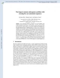
An illustration of the algorithm in work is shown in Fig. 1, where the matrix is presented in a level-wise manner. The CLCS length is located in M (r, n, m) cell. To obtain a CLCS itself, one needs to trace back the matrix according to the cells used to compute the actual cell starting from M (r, n, m), which is easy and fast [6]. k=1
k=0 i j
A B A ADACB A A BC
C 0 0 0 0 0 0 1 B 0 1 1 1 1 1 2C 0 1 1 1 1 1 3 B 0 1 1 1 1 1 0
11
j 0
1
B
B
B
2
C
2 2 2 2 2 2 2 2 2 3
1
C
1 2 2 2 2 2 2 2 2 2 2 3
1
2
2
C
2 3 3 3 3 3 2 3 3 3 3 3
3
B
3 3 3 3 3
3
B
3 3
4
D
3 3 3 3 3
4
D
3 3
2 3 4 4 4 4 2 3 4 5 5 5 2 3 4 5 5 5
5
A
5
A
3 3
6
A
6
A
3 3
7
D
3 4 4 4 4 3 4 5 5 5 3 4 5 5 5
7
D
3 3
5 5 5 5 5 6 5 5 5 5 5 6
8
C
8
C
9
D
3 4 5 5 6 3 4 5 5 6
9
D
3 4 3 4
5 6 6 6 6 6 5 6 7 7 7 7
10
B
6 6 6 6 6
10
B
6 6
11
A
6 7 7 7 7
11
A
6 6
3
3
B
3
4
D
4 5
5
A
6
A
5 5 5
7
D
5 5 6 5 5 6
8
C
9
D
6 6 6 A 1 2 3 3 4 5 5 6 7 7 7 7
10
B
11
A
A B A ADACB A A BC
0 1 2 3 4 5 6 7 8 9 10 11
1 1 1 1 1 1
1 2 2 2 2 2 2 2 2 2 2 3
D 1 1 2 3 4 4 4 4 4 8C 1 1 2 3 4 4 5 5 5 9D 1 1 2 3 4 4 5 5 5 10 B 1 2 2 3 4 4 5 6 6
i
0 1 2 3 4 5 6 7 8 9 10 11
A B A ADACB A A BC
0
2 3 3 3 3 D 0 1 1 1 2 2 2 3 3 3 3 5 A 1 1 2 2 2 3 3 3 4 4 4 6 A 1 1 2 3 3 3 3 3 4 5 5
k=3
k=2 i
0 1 2 3 4 5 6 7 8 9 10 11
C
j
1 1 1 1 1 1
4
7
i
0 1 2 3 4 5 6 7 8 9 10 11
C
A B A ADACB A A BC
j 0
C
Fig. 1. Example of the algorithm by Chin et al. for A = ABAADACBAABC, B = CBCBDAADCDBA, P = CBB. (Grayed cells denote strong matches and ‘–’ symbols denote −∞ values.)
Matrix M of this algorithm is a concept shared by some other CLCS methods, so we will be referring to it in the rest of the paper. 3.3 Peng Algorithm The algorithm by Peng [16] was invented independently, but actually is almost identical to the one by Chin et al. and can be seen as its variant, since the differences are mainly in the implementation field. The main recurrence is split according to k into two equations. For 1 ≤ i ≤ n, 1 ≤ j ≤ m: M (0, i − 1, j), M (0, i, j) = max M (0, i, j − 1), M (0, i − 1, j − 1) + 1,
if ai = bj .
5
CLCS Computing Algorithms in Practice
For 1 ≤ k ≤ r, 1 ≤ i ≤ n, 1 ≤ j ≤ m: M (k, i − 1, j), M (k, i, j − 1), M (k, i, j) = max M (k, i − 1, j − 1) + 1, M (k − 1, i − 1, j − 1) + 1,
if ai = bj , if ai = bj ∧ ai = pk .
The boundary conditions are: M (0, i, 0) M (0, 0, j) M (k, i, 0) M (k, 0, j)
= 0, = 0, = −∞, = −∞,
for for for for
0 ≤ i ≤ n, 0 ≤ j ≤ m, 0 ≤ i ≤ n, 1 ≤ k ≤ r 0 ≤ j ≤ m, 1 ≤ k ≤ r.
Finally, the CLCS length is located in M (r, n, m). 3.4 Arslan–E˘ gecio˘ glu Algorithm Another DP-based approach to solve the CLCS problem was proposed by Arslan and E˘gecio˘glu [1]. They started with the recurrence given by Tsai [19] and simplified it obtaining the following set of equations. For 0 ≤ i ≤ n, 0 ≤ j ≤ m, 0 ≤ k ≤ r: M (k, i, 0) = 0,
M (k, 0, j) = 0.
For 1 ≤ i ≤ n, 1 ≤ j ≤ m, 0 ≤ k ≤ r: M (k, i, j) = max{M 0 (k, i, j), M (k, i − 1, j), M (k, i, j − 1)}, M 0 (k, i, j) = max{M 00 (k, i, j), M 000(k, i, j)}, if (k = 0 or (k > 0 and M (k − 1, i − 1, j − 1) > 0)) M (k − 1, i − 1, j − 1) + 1 M 00 (k, i, j) = and a i = b j = pk , otherwise , 0 if (k = 0 or M (k, i − 1, j − 1) + 1 or M (k, i − 1, j − 1) > 0) M 000 (k, i, j) = and ai = b j , otherwise . 0
In this algorithm, there are more than one matrix, but the time and space complexity is still O(mnr). The CLCS length is obtained in M (r, n, m). 3.5 Peng–Ting Algorithm The first algorithm for the CLCS problem, which does not fill one or more three dimensional matrices cell by cell, was presented by Peng and Ting [17]. Their method is an example of a divide and conquer technique.
6
S. Deorowicz, J. Obst´ oj
A general scheme of the algorithm is: 1. Find the division point (k, dn/2e, j) for all 0 ≤ j ≤ m and 0 ≤ k ≤ r. 2. Compute by recurrence C1 for Adn/2e , Bj , Pk . 3. Compute by recurrence C2 for A−dn/2e , B−j , P−k . 4. Return the concatenation of C1 and C2 . A key point is to find the j and k indexes in the first step. They are computed as: arg max{M (1, k, 1, dn/2e, 1, j) + M (k + 1, r, dn/2e + 1, n, j + 1, m)}. 0≤j