This stands in stark contrast to most reported results which require either ..... pete with some data-driven supervised methods (note, SB19 needs 95% of the ...
Constrained Planar Cuts - Object Partitioning for Point Clouds Markus Schoeler, Jeremie Papon and Florentin W¨org¨otter Bernstein Center for Computational Neuroscience (BCCN) III Physikalisches Institut - Biophysik, Georg-August University of G¨ottingen {mschoeler,jpapon,worgott}@gwdg.de
ples [5, 9, 15, 18]. In this work, we aim to partition objects from the bottomup using a purely geometric approach that generalizes to most object types. This is in stark contrast to recent learning-based methods, which achieve good performance by training separate classifiers for each object class [9, 15]. While such methods do perform well on benchmarks, they are severely restricted in that one must know the object class a-priori, and they do not generalize to new objects at all. With unsupervised methods, such as the one presented in this work, there is no need to create new training data and annotated ground truth, allowing them to be employed as an off-the-shelf first step in object partitioning. While many bottom-up approaches [8, 10, 13] have been tested on the Princeton Segmentation Benchmark [5], none of them are able to achieve results comparable to human segmentations. The recent learning-free approach of Zheng et al. [18] manages results closer to the human baseline, but only by making strong assumptions about the underlying skeleton of objects. This means that the method does not work for objects where skeletonization is uninformative, and thus does not generalize well to all object classes in the benchmark. Psycho-physical studies [2, 4] suggest that the decomposition of objects into parts is closely intertwined with local 3D concave/convex relationships. It is readily observable that objects and object-parts tend to be isolated by concave boundaries. Stein et al. [14] used this idea in a bottomup segmentation algorithm LCCP, which showed state-ofthe-art performance in several popular object segmentation benchmarks. In that work, they make a strong assumption about local concavities, namely, that they completely isolate objects. While effective for object segmentation, this is problematic for more subtle part-segmentation where interpart connections may not be strongly (and/or completely) concave. For instance, in Fig.1, the shoulder only has concave connections on the underside, so a strict partitioning criterion which only cuts concave edges will not separate the arm from the torso. While it is clear that a strict partitioning will often fail
Abstract While humans can easily separate unknown objects into meaningful parts, recent segmentation methods can only achieve similar partitionings by training on humanannotated ground-truth data. Here we introduce a bottomup method for segmenting 3D point clouds into functional parts which does not require supervision and achieves equally good results. Our method uses local concavities as an indicator for inter-part boundaries. We show that this criterion is efficient to compute and generalizes well across different object classes. The algorithm employs a novel locally constrained geometrical boundary model which proposes greedy cuts through a local concavity graph. Only planar cuts are considered and evaluated using a cost function, which rewards cuts orthogonal to concave edges. Additionally, a local clustering constraint is applied to ensure the partitioning only affects relevant locally concave regions. We evaluate our algorithm on recordings from an RGB-D camera as well as the Princeton Segmentation Benchmark, using a fixed set of parameters across all object classes. This stands in stark contrast to most reported results which require either knowing the number of parts or annotated ground-truth for learning. Our approach outperforms all existing bottom-up methods (reducing the gap to human performance by up to 50 %) and achieves scores similar to top-down data-driven approaches.
1. Introduction and State-of-the-Art Segmentation of 3D objects into functional parts - forming a visual hierarchy - is a fundamental task in computer vision. Visual hierarchies are essential for many higher level tasks such as activity recognition [6, 12], semantic segmentation [1, 17], object detection [7], and human pose recognition [3, 16]. Nevertheless, part segmentation, particularly of 3D point clouds, remains an open area of research - as demonstrated by the inability of state-of-the-art methods to match human performance on existing benchmarks without excessive fitting to particular ground-truth training exam1
semantic knowledge (e.g. training or classification). As discussed earlier, local concavity is a powerful, arguably the most powerful, local feature indicative of part boundaries. In this Section we present our segmentation algorithm, which identifies regions of local concavity for a semiglobal partitioning.
2.1. Local concavity evidence extraction
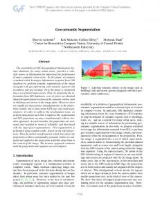
Figure 1. In complex objects parts are often only partially separated by concavities. A) Input object together with extracted Supervoxels. B) Supervoxel adjacency graph with convex/concave edge classification. C) Magnification of the shoulder showing how parts are not always strictly isolated by concave edges. While the underside of the shoulder is highly concave (suggesting a part boundary), the top of the shoulder is convex, so the arm cannot be separated from the torso by only cutting concave edges.
to separate parts, concave connections are nevertheless indicative of inter-part boundaries. In this work we use a relaxed cutting criterion which permits cuts of convex edges when nearby concave edges indicate a part boundary. To do this, we use local concavity information to find euclidean planar cuts which match a semi-global hierarchical concave boundary model. To find cuts which fit this model we propose a directionally weighted, locally constrained sample consensus scheme which, while being robust to noise, uses weights and penalties in a local model evaluation phase, leading to remarkably accurate partitionings of objects. We will show the first reported quantitative partsegmentation results on point-cloud data, results which outperform current state-of-the-art mesh-segmentation methods on the Princeton Object Segmentation benchmark and approach human ground truth segmentations. This paper is organized as follow: First, in Section 2 we propose a constrained planar cutting criterion, and describe our algorithm for finding optimal cuts. In Section 3 we evaluate our method, benchmark it against other approaches and discuss the results. Finally, Section 4 will summarize our findings. The method’s source code will be freely distributed as part of the Point Cloud Library (PCL)1 .
2. Methods Our goal is to partition point clouds into their constituent objects and object parts without the need for top-down 1 http://www.pointclouds.org
As a first step, we must find evidence of local concavities which hint at the existence of parts. We begin by creating a surface patch adjacency graph using Voxel Cloud Connectivity Segmentation (VCCS) [11], which over-segments a 3D point cloud into an adjacency graph of supervoxels (a 3D analog of superpixels). VCCS uses a local region growing variant of k-means clustering to generate individual supervoxels p~i = (~xi , ~ni , Ni ), with centroid ~xi , normal vector ~ni , and edges to adjacent supervoxels e ∈ Ni . Seed points for the clustering are initialized using a regular grid which samples the occupied space uniformly using an adjacency-octree structure. Clusters are expanded from the seed points, governed by a similarity measure calculated in a feature space consisting of spatial extent, color, and normal difference. In this work we ignore color, using only spatial distance (ws = 1) and normal difference (wn = 4) for clustering. Once we have the supervoxel adjacency graph, we use the classification proposed for the LCCP-algorithm [14] to label edges in the graph as either convex or concave. Considering two adjacent supervoxels with centroids at ~x1 , ~x2 and normals ~n1 , ~n2 we treat their connection as convex if n~1 · d~ − n~2 · d~ ≥ 0, with d~ =
x~1 − x~2 . ||x~1 − x~2 ||2
(1) (2)
Likewise, a connection is concave if n~1 · d~ − n~2 · d~ < 0.
(3)
We use a concavity tolerance angle βthresh = 10°, to ignore weak concavities and those coming from noise in the pointclouds.
2.2. Semi-global partitioning To make use of the concavity information we will now introduce a recursive algorithm for partitioning parts which can cut convex edges as well. Beginning with the concave/convex-labeled supervoxel adjacency graph, we search for euclidean splits which maximize a scoring function. In this work we use a planar model, but other boundary models, such as constrained paraboloids are possible as well. In each level we do one cut per segment from the former level (see Fig. 2). All segments are cut independently,
connects (~x1 , ~x2 ). Additionally, the points maintain the direction of the edge d~ (see Eq. (2)) together with the angle α between the normals of both supervoxels (~n1 , ~n2 ): |α| = cos−1 (~n2 · ~n1 ).
(4)
We will use α < 0 to describe convex edges and α > 0 to denote concavities using Eqs. (1) and (3). The EEC has the advantage of efficiently storing the edge information and bridging the gap between the abstract adjacency graph representation and the euclidean boundary model. 2.2.2
Figure 2. Recursive cutting of an object. Top: In each level we independently cut all segments from the former level. Red lines: Cuts performed in the level. Bottom: By changing the minumum cut score Smin we can select the desired level of granularity.
Figure 3. A chair from the Princeton Benchmark. A: Adjacency graph. B: Euclidean edge cloud extracted from the adjacency graph together with color-coded point weights ωi . C: The first euclidean planar cut splits off all 4 legs, with concavities from each leg refining the cut’s model.
that is, other segments are ignored. Cuts do not necessarily bi-section segments (as most graph cut methods), but as we cut in euclidean space, can split into multiple new segments with a single cut. This also allows us to use evidence from multiple scattered local concavities from different parts to induce and refine a globally optimal combined cut as shown in Fig. 3 C. 2.2.1
Euclidean edge cloud
An object shall be cut at edges connecting supervoxels. Consequently, we start by converting the adjacency graph into a Euclidean Edge Cloud (EEC) (see Fig. 3 B), where each point represents an edge in the adjacency graph. The point-coordinate is set to the average of the supervoxels it
Geometrically constrained partitioning
Next, we use the EEC to search for possible cuts using a geometrically-constrained partitioning model. To find the planes for cutting we introduce a locally constrained, directionally weighted sample consensus algorithm and apply it on the edge cloud as follows. While canonical RANSAC treats points equally, here we extend it with Weighted RANSAC, allowing each point to have a weight. Points with high positive weights encourage RANSAC to include them in the model, whereas points with low or negative weights will penalize a model containing them. All points are used for model scoring, while only points with weights ωi > 0 are used for model estimation. We normalize the score by the number of inliers in the support region, leading to a scale-invariant scoring. With Pm being the set of points which lie within the support region (i.e. within a distance below a predefined threshold τ of the model m ) and |x| denoting the cardinality of set x, the score can thus be calculated using the equation: Sm =
1 X ωi . |Pm |
(5)
i∈Pm
Using high weights for concave points and low or negative weights for convex points consequently leads to the models including as many concave and as few convex points as possible. In this work we use a heaviside step function H to tranform angles into weights: ω(α) = H(α − βthresh )
(6)
Please note that this will assign all convex edges a weight of zero. Still, this penalizes them in the model due to the normalization Pm of Eq. (5). The score for a cutting plane will therefore range between 0 (only convex points) and 1 (only concave points) in the support region. Simply weighting the points by their concavity is not sufficient; weighted RANSAC will favor the split along as many concave boundaries as possible. Figure 4 A shows a minimalistic object with two principal concavities, which the algorithm will connect into a single cutting plane, leading to an incorrect segmentation (Fig. 4 B). To deal with
such cases, we introduce Directional Weighted RANSAC as follows. Let ~sm denote the vector perpendicular to the surface of model m and d~i the ith edge direction calculated from Eq. (2). To favor cutting edges with a plane that is orthogonal to the edge, we add a term to the scoring of concavities: 1 X ωi ti |Pm | i∈Pm � |d~i · ~sm | i is concave ti = 1 i is convex.
Sm =
(7) (8)
The notation · refers to the dot-product and |x| to cardinality or absolute value. The idea behind Eq. (8) is that convexities should always penalize regardless of orientation, whereas concavities hint at a direction for the cutting. The effect on the partitioning is shown in Fig. 4 C. Due to perpendicular vectors |~s1 · d~1 | and |~s1 · d~2 | the directional concavity weights for the cut in B are almost decreased to zero. 2.2.3
Locally constrained cutting
The last step of the algorithm introduces locally constrained cutting. While our algorithm can use concavities separating several parts as shown in Fig. 3 C, this sometimes leads to cases where regions with strong concavities induce a global cut which will split off a convex part of the object (an example is shown in Fig. 5 B). To prevent this kind of oversegmentation we constrain our cuts to regions around local concavities as follows. Given the set of edge-points Pm located within the support region of a model, we start with a euclidean clustering of all edge-points using a cluster threshold equal to the seed-size of the supervoxels. Using n ⊂ Pm to denote the set of points in the nth cluster, we Pm modify Eq. (7) to operate on the local clusters instead of Pm : 1 X n Sm = n ωi ti . (9) |Pm | n i∈Pm
As this operation is too expensive to be employed at each model evaluation step of the RANSAC algorithm, we only apply it to the highest scoring model. Only edges with a n cluster-score Sm ≥ Smin will be cut. This whole cutting procedure is repeated recursively on the newly generated segments and terminates if no cuts can be found which exceed the minimum score Smin or if the segment consists of less than Nmin supervoxels.
3. Evaluation In this section we will describe the experimental evaluation and analysis of our proposed method.
3.1. Data sets We evaluate our algorithm quantitatively on the Princeton Object Segmentation Benchmark [5], and qualitatively on the benchmark as well as on Kinect for Windows V2 recordings. The benchmark consists of 380 objects in 19 categories together with multiple face-based ground-truth segmentations (i.e. each face in the object has a groundtruth label). In order to use a mesh annotated ground-truth to benchmark, we first create point clouds using an equidensity random point sampling on the faces of each object, and then calculate normals using the first three vertices of each face. To evaluate our segmentations, we determine the dominant segment label in the point ensemble for each face and map that label back to the face of the polygonal model.
3.2. Quantitative results We compare to the mesh-segmentation results reported in [5, 9, 18] as well as to results from LCCP[14] (with extended convexity and the sanity criteria) using the standard four measures: Cut Discrepancy, Hamming Distance, Rand Index and Consistency Error. Cut Discrepancy, being a boundary-based method, sums the distance from points along the cuts in the computed segmentation to the closest cuts in the ground truth segmentation, and vice-versa. Hamming Distance (H) measures the overall regionbased difference between two segmentations A and B by finding the best corresponding segment in A for each segment in B and summing up the differences. Depending on if B or A is the ground-truth segmentation this yields the missing rate Hm or false alarm rate Hf , respectively. H is defined as the average of the two rates. Rand Index measures the likelihood that a pair of faces have either the same label in two segmentations or different labels in both segmentations. To be consistent with the other dissimilarity-based metrics and other reported results we will use 1 − Rand Index. The fourth metric, Consistency Error, tries to account for different hierarchical granularities in the segmentation both globally (Global Consistency Error GCE) as well as locally (LCE). For further information on these metrics we refer the reader to [5]. Unlike most methods benchmarked on the Princeton Dataset our method does not need the number of expected segments as an input, allowing us to run the complete benchmark with a fixed set of parameters: Smin = 0.16, Nmin = 500 (see Fig. 6). For the supervoxels we use a seed resolution of Rseed = 0.03 and a voxel resolution Rvoxel = 0.0075. To remove small noisy segments, we also merge segments to their largest neighbor if they are smaller than 40 supervoxels. The same settings were used for LCCP, too. We denoted the degree of supervision required for the algorithms using color codes (green: unsupervised
B Global
A
stron g conc local aviti es
Figure 4. The highest scoring splits for undirectional and directional weights. A) Input object and adjacency graph. B) Using undirectional weights the best cut matches all concavities. However, this cut gets a lower score with directional weights due to the factors |~s1 · d~1 | and |~s1 · d~2 |. C) The partition when using directional weights.
Concave connections
Convex connections
Locally constrained
C
gap between clusters
Figure 5. Comparison between locally constrained and global cuts. A) Input object and adjacency graph. B) Due to the strong local concavities on the right the algorithm will cut trough a perfectly convex part of the object (left). C) Using locally constrained cuts will find two clusters (along the dashed and solid red lines). Evaluating both clusters separately will only cut the right side. All cuts used directional weights.
orange: weakly supervised and red: supervised/learning). Unsupervised methods (such as ours) do not take model specific parameters into account and use fixed parameters for the full benchmark. Weakly supervised methods need to know the number of segments. Supervised algorithms need objects from the ground-truth of each category for training, using a different classifier for every class. Despite the fact that we need to convert the mesh information to point clouds and vice-versa, our method achieves better than state-ofthe-art results on all measures. For Consistency Error and Rand Index we are able to reduce the gap for unsupervised and weakly-supervised methods to human performance by 50 %. Comparing the speed of our method to other methods, Table 1 shows that our method is competitive in terms
of complexity, too. Please note that we measured time on a single 3.2 GHz core whereas the other methods have been benchmarked by [5] on a 2 GHz CPU. Still, this allows us to estimate that our method is faster than Randomized Cuts and Normalized Cuts and about as complex as Core Extraction and Shape Diameters, while being superior in performance to all.
3.3. Qualitative results Example segmentations from the Princeton benchmark as well as Kinect for Windows V2 recordings from http: //www.kscan3d.com are depicted in Figs. 7 and 8. We should emphasize that our algorithm does not require full scans of objects, that is, it can be applied to single views
Figure 6. Comparison of proposed CPC algorithm to results published on the Princeton benchmark. Green algorithms are unsupervised, orange algorithms are weakly-supervised and red denotes supervised (i.e. training). For SB3 and SB19 [9] results on some error measures had not been published. As Zheng et al. [18] (PairHarm) did not report results on the full benchmark, we show results on their subset to the right of the dashed line. All objects have been segmented with local constrains and directional weights using fixed parameters.
as shown in Fig. 8 E. Additionally, we show the robustness of the proposed algorithm against shape variations as well as added noise in Fig. 9 using the “plier” class from the Princeton benchmark. Method Human CPC Randomized Cuts Normalized Cuts Shape Diameter Core Extraction Random Walks LCCP
Avg. Comp. Time 13.9 83.8 49.4 8.9 19.5 1.4 0.47
Rand Index 0.103 0.128 0.152 0.172 0.175 0.210 0.214 0.321
Table 1. Comparison of averaged computational time in seconds per object for the different learning-free algorithms.
4. Conclusion In this work we introduced and evaluated a novel modeland learning-free bottom-up part segmentation algorithm operating on 3D point clouds. Compared to most existing cutting methods it uses geometrically induced cuts rather than graph cuts, which allows us to generalize from local concavities to geometrical part-to-part boundaries. For this we introduced a novel RANSAC algorithm named Locally Constrained Directionally Weighted RANSAC and applied it on the edge cloud extracted from the Supervoxel Adjacency Graph. We were able to achieve better than state-ofthe-art results compared to all published results from unsupervised or weakly-supervised methods and even compete with some data-driven supervised methods (note, SB19 needs 95% of the objects for training). For Consistency Error and Rand Index we are able to reduce the gap to human performance by 50 %. We also introduced a protocol to adapt mesh-segmentation benchmarks to point clouds us-
Figure 7. Qualitative results on the Princeton benchmark. All objects have been segmented with proposed algorithm using a single set of parameters (Smin = 0.16, Nmin = 500).
Figure 8. Qualitative results for the Kinect for Windows V2 gallery recordings from http://www.kscan3d.com using proposed algorithm. A-D: Full recordings. E: Single view recording.
ing an equi-density randomized point sampling, and a backpropagation of found labels to the mesh. This allowed us to report the first quantitative results on part-segmentation for point clouds.
added Gaussian noise resulting in consistent segmentations. This means that the method is directly applicable as the first step in an automated bootstrapping process and can segment arbitrary unknown objects.
Acknowledgments The research leading to these results has received funding from the European Community’s Seventh Framework Programme FP7/2007-2013 (Specific Programme Cooperation, Theme 3, Information and Communication Technologies) under grant agreement no. 600578, ACAT.
References
Figure 9. Robustness of the segmentation against shape variations (top) and increasing noise level (bottom).
Finally, we should emphasize that our method is learning-free, which has many advantages. Most importantly, there is no need to create new training data and annotated ground truth for new objects. Additionally, learningbased methods need to know the class of an object before they can be used for segmentation, since they must select which partitioning model to use. Our method, on the other hand, can be used directly on new data without any such limitations. Despite being a purely data-driven method our algorithm can cope with shape variations and
[1] P. Arbelaez, B. Hariharan, C. Gu, S. Gupta, L. Bourdev, and J. Malik. Semantic segmentation using regions and parts. In IEEE Conference on Computer Vision and Pattern Recognition (CVPR), pages 3378–3385, 2012. 1 [2] M. Bertamini and J. Wagemans. Processing convexity and concavity along a 2-D contour: figure-ground, structural shape, and attention. Psychonomic Bulletin & Review, 20(2):191–207, 2013. 1 [3] L. Bourdev and J. Malik. Poselets: Body part detectors trained using 3D human pose annotations. In ICCV, pages 1365–1372, 2009. 1 [4] A. D. Cate and M. Behrmann. Perceiving parts and shapes from concave surfaces. Attention, Perception, & Psychophysics, 72(1):153–167, 2010. 1 [5] X. Chen, A. Golovinskiy, and T. Funkhouser. A benchmark for 3d mesh segmentation. In ACM Transactions on Graphics (TOG), volume 28, page 73. ACM, 2009. 1, 4, 5
[6] C. Desai, D. Ramanan, and C. Fowlkes. Discriminative models for static human-object interactions. In IEEE Conference on Computer Vision and Pattern Recognition Workshops (CVPRW), pages 9–16, 2010. 1 [7] A. Farhadi and M. A. Sadeghi. Phrasal recognition. IEEE Transactions on Pattern Analysis and Machine Intelligence, 35(12):2854–2865, Dec. 2013. 1 [8] A. Golovinskiy and T. Funkhouser. Randomized cuts for 3D mesh analysis. ACM Transactions on Graphics (Proc. SIGGRAPH ASIA), 27(5), Dec. 2008. 1 [9] E. Kalogerakis, A. Hertzmann, and K. Singh. Learning 3d mesh segmentation and labeling. ACM Transactions on Graphics, 29(4):1, July 2010. 1, 4, 6 [10] Y.-K. Lai, S.-M. Hu, R. R. Martin, and P. L. Rosin. Fast mesh segmentation using random walks. In Proceedings of the 2008 ACM symposium on Solid and physical modeling, pages 183–191. ACM, 2008. 1 [11] J. Papon, A. Abramov, M. Schoeler, and F. W¨org¨otter. Voxel cloud connectivity segmentation - supervoxels for point clouds. In IEEE Conference on Computer Vision and Pattern Recognition (CVPR), pages 2027–2034, 2013. 2 [12] H. Pirsiavash and D. Ramanan. Detecting activities of daily living in first-person camera views. In IEEE Conference on Computer Vision and Pattern Recognition (CVPR), pages 2847–2854. IEEE, 2012. 1 [13] L. Shapira, A. Shamir, and D. Cohen-Or. Consistent mesh partitioning and skeletonisation using the shape diameter function. The Visual Computer, 24(4):249–259, Apr. 2008. 1 [14] S. Stein, M. Schoeler, J. Papon, and F. Wrgtter. Object partitioning using local convexity. In IEEE Conference on Computer Vision and Pattern Recognition (CVPR), June 2014. 1, 2, 4 [15] W. Xu, Z. Shi, M. Xu, K. Zhou, J. Wang, B. Zhou, J. Wang, and Z. Yuan. Transductive 3d shape segmentation using sparse reconstruction. Computer Graphics Forum, 33(5):107–115, Aug. 2014. 1 [16] Y. Yang and D. Ramanan. Articulated pose estimation with flexible mixtures-of-parts. In IEEE Conference on Computer Vision and Pattern Recognition (CVPR), pages 1385–1392, 2011. 1 [17] B. Yao and L. Fei-Fei. Modeling mutual context of object and human pose in human-object interaction activities. In IEEE Conference on Computer Vision and Pattern Recognition (CVPR), pages 17–24, 2010. 1 [18] Y. Zheng, C.-L. Tai, E. Zhang, and P. Xu. Pairwise harmonics for shape analysis. IEEE Transactions on Visualization and Computer Graphics, 19(7):1172–1184, July 2013. 1, 4, 6