2007 International Conference on Intelligent Pervasive Computing
Construct intra-cluster load-balancing overlay Xuan Zhang, Xing Li ,Chongrong Li, Dongtao Liu Network Research Center, Department of Electronic Engineering Tsinghua University ,Beijing ,China
[email protected] [email protected] ,
[email protected] ,
[email protected] capacity, although not so efficient for its flooding or gossip message exchanging.Combining the advantages of the structured and unstructured overlay to achieve scalability, topology-aware and load-balancing for heterogeneous capacity nodes is our goal in the paper.
Abstract In application layer multicast, peers’ local service capacities are heterogeneous and span a large range, how to arrange the number of the node’s connections is one load-balancing issue. The other important aspect of constructing efficient overlay network is to exploit network locality in the underlying network to decrease delivery latency for media streaming. In this paper, we propose one hierarchical structure overlay, in which peers are divided into clusters according peers’ network distances. The intra-cluster nodes are self-organized to unstructured load-balancing overlay via fitness based preferential random walk. Simulation shows intra-cluster load-balancing could be gained via short walk
In this paper, we propose one hierachical overlay network, in which peer nodes are divided into clusters according network distances. The intra-cluster nodes are self-organized to unstructured load-balancing overlay via preferential random walk.
2. Related works One close work to our job is BON [8], to achieve the load-balancing, the capacity-map and degree-based random walk is proposed. Random walk now is used for sampling or locating in random graphics and P2P overlay [9][10]. The lately concerning about the nodes’ service capacity address the conflict of peer’s upload bandwidth in multiple coexisting P2PStreaming overlay [11],the game theory are used to get loadbalancing. Our wok prefers to fitness based preferential random walk way to achieve load balancing, and node clustering with locality-aware are concerned.
1. Introduction For delivering live media streaming from one or several sources to large amounts of users, native multicast is probably the most efficient way, but IP multicast is still not ubiquitous available in Internet. Recently Application Layer Multicast (ALM) is employed for media streaming[1]. By utilizing application layer user’s capability, all participate peers organize a cooperation overlay network.
3. Framework
In ALM, nodes’ local service capacities are usually heterogeneous and span a large range, how to arrange the number of the node’s connections is important for peer nodes’ load-balancing. On the other hand, how to perceive underlying network topology to decrease communication cost between peers is another issue.
3.1. Overall structure The overlay is organized as two-level hierarchy. The lower layer consists of clusters, in which one cluster super-node (SN) included. And all the super-nodes form the upper-layer, the core network. The core network are constructed as simple multicast tree such as ZigZag[2], HMTP[3]. The cluster super-nodes are deployed according to the overlay members’ location distribution. For example, we can deploy one SN in one city. So the number of the core network nodes is not too large.
The traditional ALM algorithm constructs application layer multicast tree as ZigZag[2], HMTP[3].This way is similar to network level multicast. The other structured overlay such as Chord[4],Pastry[5] construct the multicast tree by the DHT method. The unstructured overlay bases on gossip or flooding to exchange messages [6][7]. The structured overlays address scalability requirement, but are not efficient to the heterogeneous network condition or heterogeneous node’s local service capacity. Contrary, the unstructured overlay has flexibility on treating with heterogeneous nodes’
0-7695-3006-0/07 $25.00 © 2007 IEEE DOI 10.1109/IPC.2007.45
We designed the cluster-based two-level network according the general assumption: The nodes are distributed as clusters according their network distance (RTT), the inter-cluster network delays are larger than intra-cluster. The latencies of overlay peers’ could be confined to the sum of core network latency and intra-
264
cluster latency. And the two-level cluster-based structures are consistent with network-level topology and locality-aware are achieved.
4. Intra-cluster load-balancing overlay via fP-random walk 4.1 Defination and description
On the other hand, the intra-cluster peers are organized to the unstructured load-balancing overlay by preferential random walk (P-RW). We design this according the assumption: The peers’ capacity and network condition are heterogeneous and spans a large range. Here we indicate the last-mile upload bandwidth on each peer constitutes the peer’s “capacity” in the overlays [11]. When peers’ load is proportioned to their capacity, load-balancing achieved.
The intra-cluster overlay network is defined as a directed graph G(V,E) as figure 1. Vertex (V) presents peers which both receive video streaming from ancestor and disseminates streaming to children peers. Edge (E) in the graph presents actual connection or virtual connection (dashed line), edge direction is from ancestor node to child node. The overlay network is generated by peer nodes’ joining overlay sequentially.
3.2. Overlay construction
h(v3)
The overlay is constructed via two steps when one node joins the network. At the first step, the node locates the nearby cluster to join. In practice, it will locate the nearby super-node (SN) as the beginning position for random walk. When the new node locates the nearby SN, it will be designated one cluster ID as this cluster member. And the random walk will be confined to the nodes in this cluster identified by cluster ID.
v1
v4c(v4)
h(v2)
h(v5)) v5
v2 c(v2)
n- new join node v2- current step position v(1-5) -neighbosr of v2
c(v5) r(n)
n h(v) - fitness c(v)- capacity r(n)-demand bit rate
Figure 1 . Overlay definition and one step preferential random walk
Before a node join, it identifies its coordinates by using network coordinating systems. Here we implement the Hotz[12] network coordinate system. We deployed four landmark servers (X,Y,Z,K) on the network. The node n can get its coordinate Z
h(v4)
c(v1)
3.3. Node clustering
Y
v3
h(v1)
At the second step, the new node would randomly walk preferentially from the cluster SN. Via several random walks, the node will select the suitable node as the ancestor peer to achieve load-balancing.
X
c(v3)
Peer node’s properties are defined as following: a) c(x) : the upstream peer’s service capacity or available bandwidth could supply for downstream peer, the last-mile upload bandwidth on each peer in the overlays[10]. Accurately c(x) indicates the node’s current available bandwidth. Define ct (x) as c(x)
K
( d n , d n , d n , d n ) by testing its network distance d to these landmark servers. On the other hand, all cluster super-nodes’ coordinates have been tested beforehand and stored in core server.
value at time t, and c0 ( x ) as the initial capacity .
When a node n joins the network, it access the core server and get all the cluster super-nodes s coordinates and calculate the distances from n to the s. The formula of the network distance H(n,s) can be expressed as [12].
b) ht ( x ) = c t ( x ) / c 0 ( x ) : node’s fitness. The fitness presents the node’s current available capacity relate to initial capacity. h(x) is important to the preferential random walk. When t = 0, h (x) = 1;
After the calculation and comparisons, the new node will choose the super-node with smallest distance as the nearby super-node. The new node will join this cluster and get the cluster ID. At the same time, the selected super-node is regarded as the start position for intra-cluster random walk.
c) rld t ( x ) = 1 − c t ( x ) / c 0 ( x ) : relative node x at time t. Obvious rld(x)=1-h(x). .
load on
d ) r(n): When new node n joins overlay network, it demand r(n) bit rate bandwidth from ancestor node
265
e) Connect relationship: Each peer maintains three types of neighbor nodes as: ancestor, children_list and ancestor_backup. .
The leaving node’s ancestor node will delete the node from its children_list, and update its capacity and fitness similar to (2) (3) .
4.4. Metrics
4.2 Fitness based Preferential random walk
The average value of rld(x) can be presented as: Σ rld ( x ) (4) < rld >= N N The important load-balancing metric is the variance of the rld(x) represented as:
At one step walk, the walker transits from local position to one of its neighbor nodes. In Figure 1, neighbors refer to current node v2’s neighbors v(i) . The probability which neighbor node would be chosen as next walk position is proportional to neighbors’ fitness. The transfer probability in one step walk depends on the neighbor’s fitness h(v) and capacity c(v) as formula (1): hv (t ) : v ∈V , v ≠ u ∃v c(v) > r Σ v∈V ,( u ,v )∈E h(t ) v (1) 1 Pu(,hv) = v ∈ V , (u, v) ∈ E c(v) < r dv 0 (u, v) ∉ E or u = v In formula (1), line 1 means the transit probability from current peer u to its neighbor peers v is proportional to v‘s fitness h(v) when at least one neighbor’s c(v)>r(n). The two (if exist) largest h(v) nodes will be added to node set S(n) if c(v)>r(n). Line 2 means if all neighbor’s c(v)) 2 >
(5) Less the deviation and variance are, better the performance on load balancing should be.
5 Simulation and analysis The following analysis focus on two aspects: (1) Performance comparison between simple P-Random walk(sP-RW) [8] and fP-RW (2)different walk lengths.
5.1. Initialization One distribution with reciprocal law of node’s initial capacity c(x) in heterogeneous network are simulated in this paper. The reciprocal law distribution of nodes’ initial capacity could be denoted as
P (ci ( x)) ~ k / ci ( x) , k ∈ R Table I shows the initial c(x) distribution, and the number of nodes aree 12900. Here set r(n)= 0.5Mbps. For each node only makes one actual connection to ancestor, the average degree (in-degree plus outdegree) of the overlay network equals to 2. And the average load on each peer is 2*r(n) = 1Mbps. TABLE I.
c(x)/Mbps Node num P(c(x))
4.3. Peers join and depart When new node n joins overlay by connecting ancestor x at time t, capacity and fitness of peer x and n would be updated correspondingly: ct +1 ( x) = ct ( x) − r (n) (2)
ht +1 ( x) = ht ( x ) −
NODES’ INITIAL C (X) DISTRIBUTION. N =12900
30.0 9.0 900 3000 6.9% 23.3%
3.0 9000 69.8%
5.2. Compare fP-RW to sP-RW Figure 2 shows the peer nodes’ degree distribution via sP-RW way and fP-RW way from simulation results. The walk length is fixed as 10, the overlay size is 12900.
r ( n) (3) c0 ( x)
When a peer leaves the overlay, it would send message to its ancestor and children peers. Its children will select a backup ancestor peer to connect. When the backup peers’ number is below to some threshold, the node will launch a new random walk to complement the backup peers.
266
the decrease of δ(rld) is steep. When walk length is larger than 7, δ(rld) decreases smoothly. That is said, in one heterogeneous network with network size more than 10000, the effective random walk length needed is about 7. From the result, we can conclude that in our mPRW method, the relative optimized load balancing performance could be achieved with short walk length ( O(logN) ).
6. Conclusion
In this paper, we introduce one two-level hierarchical structure and intra-cluster load-balancing overlay for media streaming. We use nodes clustering to achieve low-latency according nodes’ network distances via Hotz coordinate system. The fitness based P-RW is adopted to construct unstructured loadbalancing intra-cluster overlay. Simulation shows the load-balancing performances are desirable via short length P-random walk.
Figure 2 Degree distribution on sP-RW and fP-RW method.
Table II shows the performance contrast between sP-RW and fP-RW according to figure 3.δ(rld) for sPRW equals to 0.0808 and δ(rld) for mP-RW equals to 0.0321. δ(rld) for sP-RW is twice more than fP-RW. By comparing the balancing metrics δ(rld). We can see that less variance δ(rld) is gained via fP-RW compared to sP-RW. fP-RW method performs better on load balancing than sP-RW
7. References [1]
[1]S.Banerjee,B.Bhattachargee,and C.Kommareddy. Scalable application layer multicast. In ACM SIGCOMM,August 2002. [2] D.A.Tran,K.A.Hua,and T.T.Do. Zigzag: An efficient peer-topeer scheme for media streaming.In IEEE INFOCOM,June 2003 [3] B.Zhang, S,Jamin,and L.Zhang. Host multicast:A framework for delivering multicast to end users. In IEEE INFOCOM ,June 2002 [4] I.Stoica,R.Morris, D.Karger, M.F.Kaashoek,and H.Balakrishnan. Chord: A scalable peer-to-peer lookup service for internet application. In ACM SIGCOMOM,August 2001. [5] A.Rowstron and P.Druschel. Pastry:Scalable, decentralized object location and routing for large-scale peer-to-peer systems. In IFIP/ACM International Conference on distributed System Platforms,November 2001. [6] X,Zhang, J.Liu, B.Li,and T.Yum. Data-driven overlay streaming: Design, implementation, and experience. In IEEE INFOCOM,Mar.2005 [7] A-M. Kermarrec, L. Massoulie, and A.J.Ganesh. Probabilistic reliable dissemination in large-scale systems. IEEE Transactions on Paralled and Distributed systems, 14(3):248258,2003. [8] Jesse S. A. Bridgewater, P. Oscar Boykin, Vwani P. Roychowdhury. Balanced Overlay Networks (BON): Decentralized Load Balancing via Self-Organized Random Networks .CoRR cs.DC/0411046: (2004). [9] C.Gkantsidis,M.Mihail,and A.Saberi. Random walks in peerto-peer netwroks.In IEEE INFOCOM,March 2004. [10] Aldous Fill. reversible Markov chains and random walks on graphs. http://statwww.berkeley.edu/users/aldous/RWG/book.html [11] Chuan Wu, baochun Li, Strategies of conflict in coexisting steaming overlays.IEEE INFOCOM 2007 [12] T.S Eugene Ng and HuiZhang, Predicting the Internet network distance with coordinates-based approaches, in Proceeding of INFOCOM2002,New york,June 2002.
TABLE II CONTRAST BETWEEN sP-RW and fP-RW
Methods
sP-RW
0.1945
fP-RW
0.1635
δ(rld) 0.0808 0.0321
5.3. Random walk length To find how the walk length effect on load balancing performance, we simulates 10 cases with various random walk lengths. The overlay network size and c(x) distributions are set as table I, fPRandom walk is used.
Figure 3: δ(rld) decrease when walk length increase
Figure 3 shows the simulation result about the relationship between δ(rld) and walk length. From the figure we can find δ(rld) decreases when the walk length increases. When walk length is smaller than 7,
267