IEEE TRANSACTIONS ON VISUALIZATION AND COMPUTER GRAPHICS, VOL. 15, NO. 6, NOVEMBER/DECEMBER 2009
889
Constructing Overview + Detail Dendrogram-Matrix Views Jin Chen, Alan M. MacEachren, and Donna J. Peuquet Abstract—A dendrogram that visualizes a clustering hierarchy is often integrated with a reorderable matrix for pattern identification. The method is widely used in many research fields including biology, geography, statistics, and data mining. However, most dendrograms do not scale up well, particularly with respect to problems of graphical and cognitive information overload. This research proposes a strategy that links an overview dendrogram and a detail-view dendrogram, each integrated with a re-orderable matrix. The overview displays only a user-controlled, limited number of nodes that represent the “skeleton” of a hierarchy. The detail view displays the sub-tree represented by a selected meta-node in the overview. The research presented here focuses on constructing a concise overview dendrogram and its coordination with a detail view. The proposed method has the following benefits: dramatic alleviation of information overload, enhanced scalability and data abstraction quality on the dendrogram, and the support of data exploration at arbitrary levels of detail. The contribution of the paper includes a new metric to measure the “importance” of nodes in a dendrogram; the method to construct the concise overview dendrogram from the dynamically-identified, important nodes; and measure for evaluating the data abstraction quality for dendrograms. We evaluate and compare the proposed method to some related existing methods, and demonstrating how the proposed method can help users find interesting patterns through a case study on county-level U.S. cervical cancer mortality and demographic data. Index Terms—Dendrogram, reorderable matrix, compound graphs, data abstraction quality metrics, hierarchical clusters.
1
I NTRODUCTION
A dendrogram is a form of binary tree that is typically used to visualize hierarchical relationships in data (e.g., hierarchical clustering results). A matrix is a two-dimensional graphic for displaying tabular, multidimensional data. A reorderable matrix allows permutation of data items and/or dimensions to reveal patterns of relationships, main trends, and outliers [22, 25]. A dendrogram is often integrated with a reorderable matrix, referred to as a dendrogram-matrix view here. A dendrogram-matrix view exposes patterns by leveraging perspectives of both components. This method is effective in exploring multidimensional data, helping users to generate hypotheses, to raise interesting questions and to validate knowledge. The dendogram-matrix is widely used in many research fields including biology, geography, economics, epidemiology, statistics, pattern recognition, and data mining [2, 4, 5, 12, 16, 23]. Nevertheless, standard dendrograms do not scale up well for large datasets (Figure 1, left). Large dendrograms pose both graphical rendering and human cognition problems. Occlusion of branches and leaf nodes obscures the most important features, and the resulting visual complexity quickly becomes overwhelming [15]. In addition, most traditional dendrograms provide limited support for presenting high quality contextual information to facilitate data exploration. The work described here aims to address these issues by focusing on the dendrogram component of the dendrogram-matrix. 1.1 Requirements and benefit Large datasets require new dendrogram-matrix techniques that avoid information overload and enhance scalability in both visual and cognitive aspects by (1) simplifying the graphical display while maintaining essential information and (2) providing support for easy navigation and display of contextual information. The strategies we employ to achieve this include; (1) avoiding occlusion in the display, (2) limiting the amount of information presented within any single dendrogram, (3) presenting context and focus Jin Chen is with GeoVISTA Center, Department of Geography, Pennsylvania State University, E-Mail:
[email protected]. Alan M. MacEachren is with GeoVISTA Center, Department of Geography, Pennsylvania State University, E-Mail:
[email protected]. Donna J. Peuquet is with GeoVISTA Center, Department of Geography, Pennsylvania State University, E-Mail:
[email protected] Manuscript received 31 March 2009; accepted 27 July 2009; posted online 11 October 2009; mailed on 5 October 2009. For information on obtaining reprints of this article, please send email to:
[email protected] . 1077-2626/09/$25.00 © 2009 IEEE
concurrently, and (4) supporting interactive data exploration on the dendrogram-matrix views. 1.2 Contributions The contribution of this research includes: (1) a new metric to detect skeleton in a dendrogram for constructing an abstracted, overview dendrogram, (2) a method and algorithm for dynamically constructing the overview dendrogram, (3) an enhanced measure to (emphasizing over and under abstraction) evaluate data abstraction quality for overview dendrograms, (4) a prototype of the linked dendrogram-matrix overview and detail view that meets the abovementioned requirements. 1.3 Description of this research To meet the design requirements mentioned above, we have adopted a now standard overview+detail approach. Specifically, this research proposes a strategy that separates context and focus in dynamically-linked overview and detail-view dendrograms. Similar to the concept of a compound graph by Herman, et al [15], the overview is an abstracted representation of a hierarchical cluster; it reveals the main patterns and structures inherent in the hierarchy (Figure 1, right). The overview is composed of a small selection of meta-nodes [19]; each represents a sub-tree of data elements. The meta-nodes characterize the most important features of a hierarchy, thus serves as the ‘skeleton’ of a dendrogram. Users can see the sub-tree represented by a meta-node in a detail view. This research has focused on constructing a concise overview dendrogram. We adopted an overview method conceptually similar to the one for tree visualization that was proposed in [13]. Specifically, our approach measures a metric value for each node in the original dendrogram, then ranks and selects a user-specified number of nodes as meta-nodes, and finally constructs the overview based on the meta-nodes. The proposed overview allows dynamic adjustment on the levels of detail for the entire hierarchy. To achieve high quality visual abstraction of a dendrogram, we have developed a new metric that helps to reduce information loss, and to achieve a more balanced abstraction. The rest of the paper is organized as follows. Section 2 reviews related literature. Section 3 discusses the core topics of the research including: the problems, the proposed new metric to detect the skeleton, and the algorithms for constructing an overview dendrogram. Section 4 describes our software implementation. Section 5 evaluates the proposed method, and demonstrates its usefulness via a case study on U.S. cervical cancer analysis. Finally Section 6 summarizes the method, discusses the limitations, and outlines planned future development. Published by the IEEE Computer Society
IEEE TRANSACTIONS ON VISUALIZATION AND COMPUTER GRAPHICS, VOL. 15, NO. 6, NOVEMBER/DECEMBER 2009
890
Figure 1. Left: A traditional dendrogram displaying 3105 data items. Right: The proposed overview dendrogram abstracts the data with 12 leaf nodes – total leaf count is 12. The overview allows users to dynamically adjust level of abstraction by specifying the total leaf count in the overview. The maximum leaf count can be increased via field A (currently it is 60).
2
RELATED WORK
Because our research focused on constructing a concise dendrogram overview, we have reviewed the related work in four categories: methods to reduce information overloading in dendrograms, methods for generating an overview graph, metrics to measure the node importance in an overview, and metrics to measure data abstraction quality. 2.1 Occlusion reduction in dendrograms Traditional large dendrograms display an entire hierarchy in a single view, simply compressing all the intermediate and leaf nodes into the limited display space, as shown in Figure 1(left) and in [16, 23]. It is, however, virtually impossible to display thousands of nodes without severe problems of node occlusion (also called clutter or overplotting) - nodes fitted too closely or on top of others [15]. Occlusion inhibits data exploration, pattern identification and query on individual nodes. The general methods for clutter reduction is described in [10]. Two strategies have been proposed for clutter reduction in dendrograms: focus + context, and overview + detail. The focus + context strategy merges detail and overview into a single combined view. It allows users to focus on a subset of information, while still accessing the context information (e.g., [20]). However, the strategy usually guarantees visibility for foci; causing occlusion (thus information loss) in contextual areas. Designed to avoid occlusion, the overview + detail strategy [24] suggests displaying the overview first, and zooming into a detail on demand. The strategy has been adopted in many dendrogram-matrix views [9, 16, 23]. Nevertheless, in most of these methods, the dendrogram still displays the entire hierarchy in full detail, thus still exhibiting occlusion problems. The key problem with large single-view dendrograms, whether they employ a focus + context or overview + details strategy, remains the size (i.e., the number of nodes) of the view. Data analysis becomes much easier when the view size is reduced [15]. A solution for the problem is a strategy of linked overview + detail views, which separates context and focus into an overview and a detail view. Both overview and detail views are a simplified dendrogram with reduced occlusion, measured in terms of criteria by [10]. As a result, comprehension on both contextual and detailed information is made easy. The key issue for the strategy is to construct a concise overview. The related methods are reviewed next. 2.2 Overview graph Compound graphs [21, 27] or clustered graphs[8] are strategies for providing an abstracted graph representation (i.e., an overview). A compound graph contracts sub-graphs into meta-nodes, and expands them on demand. Herman introduced a method [13, 14] to construct an overview graph he called a ‘skeleton’ – a small subset of meta-nodes that characterize the most important features of a graph. Extending this idea, Marshall et al. developed a method to
automatically build the skeleton [19]. Such techniques, however, generally focused on graphs without considering practical data analysis issues. To support pattern identification in multidimensional data, researchers integrated a matrix view with graph overview [1], and particularly with a dendrogram [2-5, 12]. This research has adopted the skeleton strategy, focusing on developing an overview dendrogram. A key issue for this strategy is to employ an appropriate metric for identifying the best metanodes. 2.3 Metric for identifying meta-nodes A metric for measuring nodes in a graph can be either count-based or distance-based. Basically, a count-based metric measures the leaf count of a node - the number of leaf nodes descending from in a node. An example is the Horton-Strahler number [17, 26] (called Strahler number henceforth). Generally, the larger the leaf count, the more complex the node is; thus meaning a larger Strahler number. Herman et al. [13] adopted the Strahler number to measures structural complexity of a tree, extract the “skeleton”, and construct an overview tree by displaying the nodes that have a metric value larger than the user-specified cut-off value. See [13, 14, 19] for examples. A distance-based metric measures the data associated with a node. In dendrograms, a node represents a merging of two clusters. Therefore, the node’s metric value is typically the Euclidean distance (dissimilarity) between the two clusters of data. The metric value can also be similarity or data variance of clusters, depending on the clustering algorithm. In dendrograms, the similarity (thus a node’s metric value) is visually reflected by the graphic distance from the node to the root in a vertical or horizontal direction (see Figure 2), so that users can focus on graphics. When displaying a large volume of data, many dendrogram-matrix views implicitly adopt this metric by abstracting a group of the low level and leaf nodes into a single node. The Hierarchical Clustering Explorer (HCE) [23] explicitly adopted this metric by providing a horizontal bar to visually set the cut-off similarity value. The entire dataset is partitioned by the sub-clusters that have the metric value immediately below the cut-off value. Figure 2 shows an implementation of the cut-off bar technique. Both count-based metrics and distance-based metrics have limits, as illustrated in detail in section 3.2. We propose a new metric particularly for dendrograms. The metric measures node count and data distance, plus a node balance factor. 2.4 Data abstraction quality metrics To evaluate data abstraction quality of an overview dendrogram, a square-error metric is usually adopted. The general objective of data clustering is to minimize within-cluster variation (commonly measured by the square-error), and thus to maximize the betweencluster variation [18]. Ward [28] uses a variation of square-error to measure information loss due to data abstraction. Cui [7] also uses square-error in a different way to measure data abstraction quality. This research adopts the square-error metric, but also emphasizes
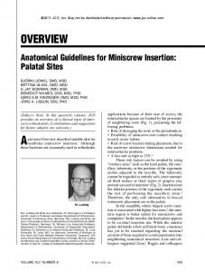
CHEN ET AL: CONSTRUCTING OVERVIEW + DETAIL DENDROGRAM-MATRIX VIEWS
cut-off bar Header
F
graphic distance to root C
B
A
891
G
HI
DE
SMR data items contained in cluster B
Figure 2. A dendrogram-matrix view implements a cut-off bar to facilitate cluster selection based on the distance-based metric. The view visualizes county-level, U.S. Cervical Cancer mortality data in five states. The data are encoded in blue-white-red colours, indicating low, normal and high mortality risk, going from blue to red, respectively. The data is currently divided into 9 sub-clusters by the cut-off bar. Cluster B is over-abstracted, and cluster F, G, H, I are under-abstracted. Cluster A contains data items with extremely low risk.
another important metric – standard deviation of square error. The second metric is important for evaluating potential over or under abstraction for overview dendrograms. 3
D ISCUSSION
OF THE PROPOSED METHOD
In this section, we discuss: (1) the data for the illustration and case study; (2) the major problems of distance-based metrics and countbased metrics that were used for constructing traditional overview dendrograms; (3) the proposed new metric; (4) the method and algorithm to construct the proposed overview dendrogram using the new metric. 3.1 The data Examples in this paper use cervical cancer mortality data for the United States between 2000 and 2004 that are publically available from the National Cancer Institute. The data are aggregated into 3,105 county and county-like enumeration units in the forty-eight contiguous states of the U.S., plus the District of Columbia. The mortality data are integrated with demographic data from the U.S. Bureau of the Census, and include the following 7 variables: Standardized Mortality Ratio (SMR), Median Household Income (Income), Percentage of Population Urbanized (P_URBAN), Percentage of Population with No Families Below Poverty (P_PNFBPOV), Percentage of Population with Families Below Poverty (P_PFBPOV), Percentage Unemployed (P_UNEMP), Percentage of Housing Units with No Vehicles Available (P_HUNVA). In the illustration cases discussed later, the 7 variables will be represented as 7 matrix rows, in the same order as listed above. The dataset is referred to as the U.S. cervical cancer and demographic dataset. The Standardized Mortality Ratio (SMR) reflects a relative risk of mortality, and is widely used in epidemiology. SMR is expressed as the ratio of observed to expected deaths. In theory, an SMR of '1' suggests normal risk, lower than '1' suggests low-risk, and larger than '1' suggests high-risk. The SMR data are highly skewed, ranging in value from 0 to 37, with a large proportion of values less than 1. In our previous study [6], the SMR is categorized into five classes: 0-0.4, 0.41-0.8, 0.81-1.2, 1.21-1.6, 1.6-37. The five classes are encoded in a specially-designed divergent color scheme, and are interpreted as: low risk (blue), low-to-medium risk (light blue), normal risk (white), medium to high risk (light red), high risk (red). 3.2 The problem One goal for the overview dendrogram introduced here is to achieve a minimum amount of information loss at a user-specified level of data abstraction. A second goal is to achieve balanced data abstraction quality across the meta-nodes in the overview, avoiding over-abstraction for some meta-nodes and under-abstraction for the others. Achieving these goals requires an appropriate metric for extracting the skeleton of a dendrogram. Below, we illustrate the
problems of both count-based and distance-based metrics in achieving the goals, and emphasize the importance for balanced data abstraction. We use a subset of U.S. cervical cancer data that includes 421 counties from five contiguous states in the southeast (U.S.: Mississippi, Alabama, Georgia, South Carolina, and Florida). The data subset contains only a single variable - SMR. A dendrogram-matrix overview using a distance-based metric alone suffers from a large information loss and unbalanced abstraction because the metric does not measure the number of data items represented by a node. As illustrated in Figure 2, a cut-off line graphically specifies a metric value in terms of the graphic distance to root. The nodes having values immediately below the cut-off value are abstracted as a single leaf node in the overview. The leaf nodes represent 9 clusters (A, B, C, D, E, F, G, H). The metric does not consider data count of the clusters, thereby inappropriately considering tiny clusters F, G, H, I as equally important as large cluster B. Consequentially, the over-abstracted node B, which could be broken into smaller pieces, contains too many data items (+280); while under-abstracted nodes (e.g., F, G, H, I) contain too few data items (around 1-3 items), which could be abstracted as a single leaf node. In practice, under-abstracted nodes increase the number of meta-nodes (thus complexity) in the overview, without providing much useful information; and overabstracted node suffer large information loss. For example, the over-abstracted node B would represent 280 data items ranging in SMR from 0.2 to 2.0, covering all five classes. Because node B cannot be categorized in any of the five classes, information is lost for the 280 data items in the overview. An overview dendrogram-matrix using a count-based metric alone would also suffer from the unbalanced-abstraction problem. An illustration is provided in section 5. Overview with unbalancedabstraction generally suffers more overall information loss than a balanced overview. Therefore, a better metric for constructing a dendrogram-matrix overview would be one that measures both distance (thus data variance) and node count, and maintains a more balanced abstraction, as discussed next. 3.3 The metric This research presents a metric that measures a node’s importance in terms of three features: (1) leaf count (thus data elements) of a node, (2) node balance – the difference in leaf count between the node’s two children, and (3) information saved– the decrease in data variance if a node is selected as a meta-node, which is kept ‘open’ to display its two children (as detailed in section 3.4). Put another way, a meta-node avoids an increase in data variance (thus information loss) that would otherwise be caused by ‘closing’ that node. We name the metric the CIB metric – denoting the three key features: count, information, and balance. The value of node K in a dendrogram is defined as M (K), as expressed below:
info
(1)
IEEE TRANSACTIONS ON VISUALIZATION AND COMPUTER GRAPHICS, VOL. 15, NO. 6, NOVEMBER/DECEMBER 2009
892
B
D
A
E C
Figure 4. Node A is not balanced – B has much more leaf nodes than C. Node B is more balanced – D, E have similar leaf nodes
where is the leaf count of the left sub-node, is the leaf count of the right sub-node. measures leaf count and node balance; infosave (k) denotes the information saved at node k. The greater the value of a node, the more likely it would be chosen as a meta-node. The metric is explained in detail below. Count-based metrics that measure leaf count of a node are common methods for measuring the complexity of the node in a tree, as already discussed in section 2.3. Generally, the larger the leaf count, the more complex the corresponding sub-tree. Adopting this idea, the proposed metric also measures a node’s complexity in terms of its leaf count, but in a slightly different way. In the metric, ( produces a larger value given a larger leaf count ( , and produces the maximum value when is equal to . Hence, ( measures both the leaf count and the node balance. Measuring the node balance is important. When determining meta-nodes, a more balanced node is preferred over a less balanced one. This is because a meta-node will be kept ‘open’ – displaying its two children, and thus visually emphasize the separation of two distinct clusters of data. This is particularly true when both are of considerable size; while an unbalanced meta-node could separate only a large cluster from a tiny cluster. As shown in Figure 3, it makes more sense to select balanced node B as a meta-node rather than unbalanced node A, since if A were a meta-node, then B would be “closed”, which would in-turn cause loss of the information on two distinct clusters: D, E. The proposed metric extends the way of distance-based metrics in measuring data variance. Data variance is usually measured in terms of thematic distance (e.g. Euclidean distance) in attribute space, or other more complex measurements such as a Nearest Neighbor Measure as proposed in [7]. Choosing an appropriate data-variance measurement is beyond the discussion of this paper. On the other hand, in a dendrogram, the height of an intermediate node – graphic distance to the bottom (see Figure 4) – visually expresses the thematic distance (or dissimilarity) between the two child clusters. To reduce dependency on the underlying clustering algorithms, we simply measure the graphic distances between a node and its two child nodes – to reflect the increase in data variance (thus information loss) due to the merging. In the equation (1), infosave(k) can be considered as a weighted, virtual distance between a node K and its two children, which is calculated below: ,
,
(2)
, is the graphic distance along one dimension ( horizontal or vertical) from node k to its left child l , and , is the distance from node k to its right child r, as shown in Figure 4. The distance is weighted by the percentage of a node’s leaf count to its parent’s leaf count – i.e., / . Since it measures more features of dendrograms, the CIB metric can outperform count-based and distance-based metrics considerably when the hierarchical structure is “unbalanced” consists of unbalanced nodes that have two direct sub-nodes with considerably different leaf count and/or data variance (e.g., unbalanced node A and balanced node B in Figure 3). Figure 7 is also an example of unbalanced structure. The CIB metric would
Figure 3. Node height and dist () - graphic distance
achieve similar results as the other metrics when a hierarchical structure is very “balanced”. The claim is supported in section 5. 3.4 Algorithms for constructing the overview In contrast to the traditional overview graph that ‘close’ a metanode by abstracting it as a leaf node; our dendrogram-matrix overview keeps a meta-node ‘open’ to display its two direct child nodes, while abstracting each child node as a leaf node if it is not a meta-node. This strategy allows a meta-node to visually reflect information saving and node balance that are measured by the CIB metric. Accordingly, the data items contained in the cluster represented by the leaf node are aggregated as a mean vector, which is displayed as a matrix column. The overview allows users to specify the number of meta-nodes via a slider bar, which determines the total leaf count – the total number of leaf nodes displayed on the overview (under the root node)(Figure 1, right). Given a total leaf count, meta-nodes can be easily detected by following the four steps below: (1) measure the ‘importance’ for each node in the original dendrogram, based on the CIB metric; (2) sort all the intermediate nodes by the metric values, put more important nodes in front of a list; (3) set the root node as the first one in the list, (4) select the most important P nodes in the list as the meta-nodes. Given the P meta-nodes, the abstraction algorithm for constructing the overview is described as below: (1) clone the original dendrogram; (2) sort the P meta-nodes based on their graphic distance to root; (3) starting from the meta-node with the largest graphic distance to root, traverse the cloned dendrogram from the bottom to the top; (4) if a meta-node is found, abstract any of the two children nodes as a leaf node if the children node is not a meta-node;(5) search through all the parents of the current metanode, to find the next meta-node; (6) go through steps from 2 to 6 until the root node is reached. 4
I MPLEMENTATION
The proposed metric and matrix overview has been implemented in the visual inquiry toolkit (VIT) [4, 5], developed and implemented by Jin CHEN using the Java Swing library, and GeoVISTA Studio – an open source Java framework. The VIT implements several classic hierarchical clustering algorithms including average-link, single-link, complete link, and Ward’s method [18]. In addition, some spatially-constrained hierarchical clustering algorithms have been developed and implemented. VIT provides a graphic user interface for users to choose a subset of variables, and their weights, on which the clustering is based. To generate an overview, a user simply needs to specify the total leaf count by dragging a slider bar on the top (Figure 9). The maximum leaf count can also be specified. Once generated, the overview presents the SSE and Std (SSE). The overview component is dynamically linked to the detail view component, so that if the user clicks on a leaf node in the overview, the detail view automatically zooms to display the corresponding sub-cluster represented by the leaf node. The detail view also highlights each of
CHEN ET AL: CONSTRUCTING OVERVIEW + DETAIL DENDROGRAM-MATRIX VIEWS
the sub-clusters with a green circle for the corresponding meta-node in the overview. The overview offers a visual cue via branch width – a wider branch contains more data items. The matrix headers also display the number of data items contained in each leaf node (Figure 6). The exploration strategy is to look at the overview first, adjust abstraction level, quickly identify more viable patterns, and then investigate the patterns in the detail view. The goal is to identify association among variables, as demonstrated in section 5.2.2. While rendering performance is not the focus of this research, our current implementation supports real-time interaction on a hierarchy with a total leaf count of 3000+. Our algorithms allow quick detection of meta-nodes and construction of the overview – it takes less than 1 second for the U.S. cervical cancer subset, and 1-2 seconds for the full dataset, all experimented on a Dell M4400 laptop. Our future work will optimize on the algorithms. 5
E V ALU ATE
THE OVERVIEW DENDROGRAM - M ATRIX
We evaluate the overview dendrogram-matrix in two ways. First, we quantitatively measure data abstraction quality on the overview, and compare the CIB metric with the count-based and distancebased metrics. Second, using the U.S. cervical cancer mortality data, we qualitatively examine data abstraction performance. This includes a case study to demonstrate how the proposed dendrogram-matrix views facilitate finding interesting patterns in comparison with HCE. Finally we qualitatively evaluate the scalability of the proposed method. 5.1
Quantitative evaluation on abstraction quality
5.1.1 Quantitative evaluation design To quantitatively evaluate data abstraction quality for overview dendrograms, this research use both sum-square-error (SSE) and its standard deviation (Std (SSE)). Measuring SSE is a common evaluation method, as discussed in section 2.4. The square-error of a cluster is the Euclidean distance between the cluster’s center and its data items. Here, the square-error is also referred to as leaf-node error, indicating the error of a leaf node that represents the cluster in the overview. A leaf node that represents only a single data item has the square-error of 0. The SSE is the sum of leaf node errors in the overview. A small SSE value indicates high abstraction quality, at a given total leaf count. Std (SSE) evaluates the variation of data abstraction quality among the leaf nodes in an overview. At a given level of abstraction, an extremely large leaf-node error indicates a leaf node has been over-abstracted, while a leaf-node error of 0 (or extremely small values) indicates under-abstraction. A small Std (SSE) indicates low occurrence of over or under abstraction. Our evaluation compared CIB with count-based and distancebased metrics, focusing on their application in unbalanced hierarchical structure. The structure is a typical result from clustering highly skewed data, common in many domains. The
893
structure can also be an artifact generated from particular clustering algorithms. Examples of such algorithms are a single-link clustering algorithm that can cause chain effects in the clusters, or a spatiallyconstrained clustering algorithm that allows two clusters to merge only if the two regions they represent are geo-spatial neighbors. Average-link and Ward algorithms tend to produce more balanced structures. The evaluation used three datasets: the U.S. cervical cancer dataset, a skewed simulated dataset, a simulated dataset in relatively normal distribution, using the average-link algorithm by default, which does not favor a specific metric. 5.1.2 Quantitative evaluation result Figure 5 shows the comparison of SSE between the CIB and distance-based metrics, using the U.S. cervical cancer sub dataset (421 counties). The result was obtained for a series of 13 abstraction levels – with the total leaf count ranging from 3 to 15. The overview using CIB metric has considerably lower error than one using the distance-based metric, particularly at a high level of abstraction when the total leaf count is small. When the abstraction level is lower (e.g., 20 nodes to represent 421 data items), the error difference becomes small. In addition, the error decreases more smoothly for the proposed metric as the total leaf count is increased. This helps to avoid accidental information loss due to an inappropriate abstraction level chosen by users. Figure 5 also shows that the Std (SSE) obtained by using the CIB metric is much lower than that by using the distance-based metric at the high level of abstraction, indicating the CIB metric can achieve a more balanced abstraction. We compared CIB with a count-based metric using the same dataset as above and a relatively-normally-distributed, simulated dataset. The two results are close due to the relatively balanced hierarchical structure. Then we applied a single-link algorithm to produce a more unbalanced structure. The CIB metric produced noticeably lower SSE and Std (SSE). In addition, we applied an average-link algorithm on the highly skewed simulated data that was generated using the Random function in Microsoft Excel. Most values for the resulting data ranged from 0 to 10, with a few from 10 to 100. CIB metric achieves much lower SSE and Std (SSE) than the count-based metric. Figure 5 (right) shows this comparison on SSE. In summary, all these measures suggest higher abstraction quality for the CIB metric than the others. 5.2 Qualitative evaluation on abstraction quality We first demonstrate the dendrogram-matrix overview and the corresponding detail view using the five-state subset of U.S. dataset, and compare the detail view with one using the distancebased metric (Figure 2). Then, we compare the proposed method with HCE, using the full U.S. cervical cancer and demographic data. 5.2.1 Comparison of metrics When analyzing the five-state subset, we set the total leaf count to 9
Figure 5. Quantitative evaluation. Left and middle plots compare SSE and Std(SSE) between the CIB (blue) and distance-based (red line) metrics. The right plot compares SSE between the CIB (blue) and count-based (red line) metrics. The metric values were measured at a series of abstraction levels from the total leaf count of 3 to 20 in the overview.
IEEE TRANSACTIONS ON VISUALIZATION AND COMPUTER GRAPHICS, VOL. 15, NO. 6, NOVEMBER/DECEMBER 2009
894
Figure 6. Qualitative evaluation. The dendrogram-matrix overview (left) and detail view (right) visualize the U.S. cervical cancer mortality for the five states. Equipped with the proposed metric, the overview divides the data into 9 clusters with much less within-cluster variance than that shown in Figure 2. The detail view shows no obvious under-abstraction (e.g. leaf node representing a single data item) or overabstraction (e.g., a cluster covering multiple colors). The 9 clusters in this figure reasonably represent various levels of mortality risk.
nodes in the overview (Figure 6, left). The 9 leaf nodes represent 9 clusters (A, B, C, D, E, F, G, H, I) the detail view (Figure 6, right). By comparing Figure 2 with Figure 6, we found that clusters A, C, D, E in Figure 2 are the same as clusters A, F, G, H in Figure 6. However, the proposed method further partitions cluster B in Figure 2 into clusters B, C, D, E, in Figure 6, therefore avoids overabstraction. On the other hand, the method combines clusters F, G, H, I in Figure 2 into cluster I in Figure 6, thereby avoiding underabstraction. By avoiding unbalanced abstraction, the method reduces information loss. The proposed overview has a SSE of 49.2 and a standard deviation of leaf-node error of 3.4 at the abstraction level of 9 nodes (Figure 5). Both measures are much lower than those measured from the sub-clusters in Figure 2 (104.6, 29.3 respectively). The benefit is reflected in real-life data analysis. For example, the four clusters (B,C,D,E) in Figure 6 represent data groups that correspond to the four classes of mortality risk (SMR): low-to-medium risk (light blue), normal risk (slight blue, white, and slight red), medium to high risk (light red), and high risk (red). The four clusters thus offer much more meaningful information than cluster B in Figure 2, which abstracts the same data items but provides little information on the mortality risk. Similarly, the cluster I in Figure 6 covers SMR from 5.8 to 11.1, which represents a cluster of counties with extremely high risk. It makes more sense to abstract the data into cluster I rather than the four clusters (F, G, H, I) in Figure 2. 5.2.2 Comparison to HCE – a case study Next, we illustrate how our dendrogram-matrix views can help to identify interesting patterns. We compare our method to HCE, because it is well-known and publicly available. We use the full U.S. cervical cancer and demographic dataset containing 3105 data items and 7 variables. The data items are represented as columns; and the variables are represented as rows in the matrix, listed in the same order as section 3.1 (e.g., SMR is in the first row). The hierarchical structure is “unbalanced”. HCE compresses and displays the entire dataset in the display view (Figure 7). When the cut-off bar is set to partition the data into 20 clusters, we find cluster A contains a large number of data items (probably over 2000) and has a large data variance. Such huge clusters are found at other abstraction levels (e.g., a partition of 46 clusters). The clusters are obviously over-abstracted, and do not expose any useful patterns in that portion of the data, particularly as shown in the mortality ratio (SMR) row. On the other hand, clusters represented by E are very small, and hence under-abstracted. Severe occlusion is also seen across all the clusters. Furthermore, interactively exploring clusters is very difficult because users need to select any cluster as a whole to display it in the detail view. Cluster A contains too many data items to be fully displayed in the detail view. Even when we set the cut-off bar to show 105 clusters, huge clusters are still seen on the left and in the middle. In summary, HCE provides limited support for analysis of these highly skewed data that are common in many domains (e.g., public health and demography). Our dendrogram-matrix views can help identify associations of high mortality with potential co-variates. When the total leaf count
is set to 40, the overview reveals several interesting patterns – e.g., pattern A and B (Figure 8, left). The columns in both patterns have the first row in red, and third row in blue. Pattern A suggests that an association between high mortality risk (i.e., red in first row) and low percentage of urbanization (i.e., blue in the third row) potentially existed in the counties of the clusters. To avoid ecological fallacy, we need to investigate the individual counties. We selected the 4 columns in the overview, and displayed the 4 clusters (C, D, E, F) in the detail view. Figure 8 shows that the pattern persists in the detail view, providing further evidence for the association. In addition, pattern A suggests weak (or maybe no) association between mortality and affordability of health service in these counties; no obvious patterns are seen for income and unemployed rate variables, as indicated by inconsistent colors across the columns. As a result, a hypothesis can be generated that high mortality is more related to availability than affordability of health services in these counties. If the counties are adjacent, then the hypothesis suggests geographical disparity for diseases and risk factors. Identifying disparity is particularly valuable for analysis of a disease and its risk factors as emphasized by the National Cancer Institute [11]. To confirm the hypotheses, spatial data analysis (e.g., spatial clustering and statistics) must be employed; and data related to health services availability may need to be collected. The case study also demonstrated that, at different levels of abstraction, the proposed method achieves much more balanced abstraction than HCE – all the nodes represent clusters with size less than 200 data items; the size is quite manageable in the detail view. In contrast, with the cut-off bar technique, unmanageably large clusters (e.g., size of more than 1000 data items) are constantly found at various levels of abstraction. 5.3 Qualitative Evaluation on scalability The proposed method can dramatically increase the scalability of the dendrogram-matrix view. The overview can easily display over 100 leaf nodes, each taking 10-20 pixels in width ( as shown in Figure 9, top plot). The overview guarantees no occlusion, and presents a clear matrix view for pattern identification, and supports easy navigation through the hierarchy. The detail view can clearly display around 400-450 nodes on an ordinary 1900*1200 screen, with each node taking 4 pixels in width (as shown in Figure 9, bottom plot). The detail view not only avoids occlusion, but also offers the capacity to detect patterns, and query on any individual data item on the screen. Dynamically linked, the overview and detail view can, in theory, support exploring large datasets of around 40,000 data items, with context and focus concurrently displayed, and no occlusion. In practice, a high performance detail view to quickly zoom and render a sub dataset is essential to achieve scalability. High performance rendering is beyond the scope of this research, which focuses on constructing concise overview to avoid information overloading and occlusion. To summarize the evaluation, the proposed dendrogram-matrix method provides enhanced overall scalability, high quality of data abstraction in terms of information loss and balance, and avoids occlusion.
CHEN ET AL: CONSTRUCTING OVERVIEW + DETAIL DENDROGRAM-MATRIX VIEWS
895
E cluster A B
C
D
SMR
SMR
SMR Figure 7 U.S. cervical cancer and demographic data displayed by HCE. The first matrix row is the SMR variable. In the top plot, the cut-off bar sets a similarity level dividing the data into 20 clusters. Cluster A is obviously over-abstracted, and clusters denoted by E are underabstracted. In the 2 bottom plots, the cut-off bar divides the data into 46 and 105 clusters. To save space, fewer rows are displayed here. Over-abstraction is seen in many clusters on the left, and under-abstraction on the right side. Occlusion is observed in most clusters.
C
1 3
D
E
F 1 2 3 4 5
6
7
A
B
Figure 8. U.S. cervical cancer and demographic data displayed by the proposed method. The overview (left plot) shows a pattern A including 4 columns. The 4 clusters all have the first row in red, indicating high mortality risk (SMR) in these counties. The clusters also have the third rows in blue, indicating very low percent of urbanization in the counties. The detail view (right plot) shows individual counties of the 4 clusters (C, D, E, F). Most counties of the clusters have high SMR (i.e., first row in red) and low urbanization (i.e., third row in blue).
Figure 9. The dendrogram-matrix views display the U.S. cervical cancer and demographic data. The overview summarizes the data in a finer level of detail, in 105 nodes. The detail view displays over 400 data items, and highlights 188 counties belonged to the 8 selected clusters in the overview. The 188 counties were previously represented as the 4 clusters in the overview shown in Figure 8.
IEEE TRANSACTIONS ON VISUALIZATION AND COMPUTER GRAPHICS, VOL. 15, NO. 6, NOVEMBER/DECEMBER 2009
896
6
C ONCLUSION
Traditional large dendrogram-matrix techniques suffer both visual rendering and human cognition problems that include (1) occlusion, which results when a large number of visual elements are displayed in a limited screen space, (2) poor viewability - i.e., many nodes and branches are barely visible, (3) poor utility - i.e., nodes, braches and matrix cells offer few useful insights due to information overload and human perceptual capacity that can discern a limited number of nodes and edges at a time. In addition to the well-known scalability issue for dendrograms, this research reports and illustrates unbalanced abstraction issues in overview dendrograms. In our work to address the issues mentioned above, we have proposed and developed an approach that is equipped with a dendrogram-matrix overview linked dynamically to a detail view and a new metric to measure importance of nodes. The proposed method provides: (1) enhanced scalability for easily exploring relatively large datasets, (2) elimination of occlusion with a relatively large dataset, (3) manageability of information for the overview and the detail view, (4) concurrent access to both context and focus, and (5) high quality of data abstraction in terms of information loss and balance. The proposed method has applications in many research fields as mentioned in the introduction. The method provides an enhanced way to analyze large multidimensional datasets. It helps to identify patterns, generate hypotheses, and pose new questions. A disadvantage of the method is that: users need to switch between the overview and detail views, costing increased cognition effort. Further research will focus on strategies to reduce the cognitive cost of using linked views. 7
A CKNOWLEDGMENTS
This work is supported in part by the US Department of Homeland Security through the Northeast Visualization and Analytics Center (NEVAC) and by the National Cancer Institute under grant R01 CA95949-01. R EFERENCES [1.] J. Abello and F. van Ham, “Matrix zoom: A visual interface to semiexternal graphs,” Proc. Information Visualization, 2004. INFOVIS 2004. IEEE Symposium on, 2004, pp. 183-190. [2.] A.A. Alizadeh, et al., “Distinct types of diffuse large b-cell lymphoma identified by gene expression profiling,” Nature, vol. 403, no. 6769, 2000, pp. 503-511. [3.] Z. Bar-Joseph, et al., “K-ary clustering with optimal leaf ordering for gene expression data,” Bioinformatics, vol. 19, no. 9, 2003, pp. 10701078. [4.] J. Chen and A.M. MacEachren, “Resolution control for balancing overview and detail in multivariate spatial analysis,” Cartographic Journal, The vol. 45, 2008, pp. 261-273. [5.] J. Chen, et al., “Supporting the process of exploring and interpreting space-time, multivariate patterns: The visual inquiry toolkit,” Cartography and Geographic Information Science, vol. 35, no. 1, 2008, pp. 33-50. [6.] J. Chen, et al., “Geovisual analytics to enhance spatial scan statistic interpretation: An analysis of u.S. Cervical cancer mortality,” International Journal of Health Geographics, vol. 7, no. 1, 2008, pp. 57. [7.] Q. Cui, et al., “Measuring data abstraction quality in multiresolution visualizations,” Visualization and Computer Graphics, IEEE Transactions on, vol. 12, no. 5, 2006, pp. 709-716. [8.] P. Eades and Q.-W. Feng, “Multilevel visualization of clustered graphs,” Graph drawing, 1997, pp. 101-112. [9.] M.B. Eisen, et al., “Cluster analysis and display of genome-wide expression patterns,” Proc. Nat'l Academy of Science, vol. 95, no. 25, 1998, pp. 14863-14868.
[10.] G. Ellis and A. Dix, “A taxonomy of clutter reduction for information visualisation,” Visualization and Computer Graphics, IEEE Transactions on, vol. 13, no. 6, 2007, pp. 1216-1223. [11.] H. Freeman and B. Wingrove, Excess cervical cancer mortality: A marker for low access to health care in poor communities, National Cancer Institute, Center to Reduce Cancer Health Disparities, 2005. [12.] D. Guo, et al., “A visualization system for space-time and multivariate patterns (vis-stamp),” IEEE Transactions on Visualization and Computer Graphics vol. 12, no. 6, 2006, pp. 1461-1474. [13.] I. Herman, et al., “Tree visualisation and navigation clues for information visualisation,” Computer Graphics Forum, vol. 17, no. 2, 1998, pp. 153-165; DOI doi:10.1111/1467-8659.00235. [14.] I. Herman, et al., Skeletal images as visual cues in graph visualization, CWI (Centre for Mathematics and Computer Science), 1998. [15.] I. Herman, et al., “Graph visualization and navigation in information visualization: A survey,” Visualization and Computer Graphics, IEEE Transactions on, vol. 6, no. 1, 2000, pp. 24-43. [16.] M. Hibbs, et al., “Viewing the larger context of genomic data through horizontal integration,” Proc. Information Visualization, 2007. IV '07. 11th International Conference, 2007, pp. 326-334. [17.] R.E. Horton, “Erosioned development of systems and their drainage basins, hydrophysical approach to quantitative morphology,” Bull. Geol. Soc. America, vol. 56, no. 1945, 1945, pp. 275-370. [18.] A.K. Jain and R.C. Dubes, Algorithms for clustering data, Prentice Hall, 1988, p. 320. [19.] M.S. Marshall, et al., Automatic generation of interactive overview diagrams for the navigation of large graphs, CWI (Centre for Mathematics and Computer Science), 2000. [20.] T. Munzner, et al., “Treejuxtaposer: Scalable tree comparison using focus+context with guaranteed visibility,” Book Treejuxtaposer: Scalable tree comparison using focus+context with guaranteed visibility, Series Treejuxtaposer: Scalable tree comparison using focus+context with guaranteed visibility, ed., Editor ed.^eds., ACM, 2003, pp. [21.] M. Raitner, “Visual navigation of compound graphs,” Graph drawing, 2005, pp. 403-413. [22.] C. Schmid and H. Hinterberger, “Comparative multivariate visualization across conceptually different graphic displays,” 1994, pp. 42-51. [23.] J. Seo and B. Shneiderman, “Interactively exploring hierarchical clustering results,” Computer, vol. 35, no. 7, 2002, pp. 80-+. [24.] B. Shneiderman, “The eyes have it: A task by data type taxonomy for information visualizations,” Proc. Proceedings of the 1996 IEEE Symposium on Visual Languages 1996, pp. 336-343. [25.] H. Siirtola and E. Makinen, “Constructing and reconstructing the reorderable matrix,” Information Visualization, vol. 4, 2005, pp. 3248. [26.] A.N. Strahler, “Hypsometric (area-altitude) analysis of erosional topography ” Geological Society of America Bulletin, vol. 63, no. 11, 1952, pp. 11171142. [27.] K. Sugiyama and K. Misue, “Visualization of structural information: Automatic drawing of compound digraphs,” Systems, Man and Cybernetics, IEEE Transactions on, vol. 21, no. 4, 1991, pp. 876-892. [28.] J.H. Ward, Jr., “Hierarchical grouping to optimize an objective function,” Journal of the American Statistical Association, vol. 58, no. 301, 1963, pp. 236-244.