Constructive heterogeneous object modeling using signed

Constructive heterogeneous object modeling using signed approximate real distance functions Pierre-Alain Fayolle, Alexander Pasko, Benjamin Schmitt, Nikolay Mirenkov The University of Aizu, Department of Information Systems Hosei University Computer Graphics Research Institute and Hosei University, Digital Media Professional The University of Aizu, Department of Information Systems

ABSTRACT We introduce a smooth approximation of the min / max operations, called SARDF (Signed Approximate Real Distance Function), for maintaining an approximate signed distance function in constructive shape modeling. We apply constructive distance-based shape modeling to design objects with heterogeneous material distribution in the constructive hypervolume model framework. The introduced distance approximation helps intuitively model material distributions parameterized by distances to so-called material features. The smoothness of the material functions, provided here by the smoothness of the defining function for the shape, helps to avoid undesirable singularities in the material distribution, like stress or concentrations. We illustrate application of the SARDF operations by two- and three-dimensional heterogeneous object modeling case studies.

Keywords Constructive heterogeneous object modeling, distance function approximation, set-theoretic operations, Function Representation (FRep).

1

INTRODUCTION

Solid modeling methods have mostly focused so far on developing models that capture only the geometry of objects, under the assumption that most of them are homogeneous. Recently, a particular attention has been paid to heterogeneous objects modeling, where an object has a number of non-uniformly distributed attributes assigned at each point and varying in space. These attributes may or may not be continuous and have different nature such as photometric characteristics, material density or distribution, physical properties, and others. Heterogeneous objects are widely used in different areas of design and engineering such as rapid prototyping, physical simulations, geological and medical modeling. We provide in this work new functional definitions for the set-theoretic operations to be used in constructive distance-based modeling of heterogeneous objects. These functions provide a smooth controlled

approximation of min / max used traditionally in constructive modeling of distance fields ([1,2]). In the present work, we try to propose an answer to the question on how can one practically construct heterogeneous objects where the material distributions are parameterized by the distance to material features.

1.1 1.1.1

Previous works Heterogeneous modeling

Several techniques for modeling heterogeneous objects are already available, presenting some noticeable analogies with homogeneous object modeling. Existing homogeneous object models include surface representations (boundary representation, feature based models); and volumetric representations (voxel arrays, adaptive spatial decompositions, function representation, etc). Each homogeneous model has been extended to allow for the underlying model to handle heterogeneity. R-sets are considered as a basis for modeling and are extended for material inclusion in [3]. An object is subdivided in components; each of them is homogeneous inside and has an assigned material index. Set-theoretic operations can be applied to the solid’s components with the corresponding operations on the material. Unfortunately, this modeling technique is limited to the representation of discretely varying material properties. In [4], a more general model is proposed: the geometry is represented by the point set decomposition into a finite set of closed 3-cells, whereas the attributes are defined by a collection of functions, which map the object geometry to several attributes. Such a mathematical model is known as a fiber bundle, with the geometrical model playing the role of the base space. Several other works are using the same model, extending it in various directions ([5,6]). However, as noticed in [7], this model does not really offer concrete computational solutions. Volumetric representations naturally define solids: a homogeneous object can be defined as a subset of the 3D space, with an additional scalar value given at any point. In the case of a spatial enumeration, like voxels [8], extension to heterogeneity consists in adding a scalar value for each attribute [9]. The drawback of this method

is the difficulty to directly describe the material distribution, without using a data acquisition device (therefore it is supposed that the object to be modeled already exists). Furthermore, the discrete property of the model requires some special approximation procedures. In [10], a general mathematical framework for modeling heterogeneous objects is proposed. An object is defined as a multidimensional point-set in space; its geometry is characterized by a signed real function at least continuous [11]; different attributes are also defined by functions and their domains of definition. In this framework, the domain of definition of an attribute is called a space partition. Both the geometry and the space partitions of the object can be defined by constructive modeling, using either the general R-functions [12], or min / max functions [1,2]. However, the problem of parameterization and control of attributes in the case of material modeling is left unanswered. A continuous volumetric representation was proposed in [13], where a B-spline volume is used to model the object geometry, whereas the attributes are modeled by means of diffusion. This model seems to suffer from the lack of flexibility of the geometry limited to volume splines. Biswas et al. [7] are interested in the representation and control of material distributions by some intuitive parameters related to the geometry of the solid and/or its material features for meshfree modeling. They propose to use the distance functions from material features (point-sets of any dimension with known material properties) as these parameters. It appears from the existing literature that the (Euclidean) distance, or functions of the distance function are indeed the most common types of material functions constructed by methods based on spatial discretization [14,15,16]. The authors of [7] demonstrate that this approach is theoretically complete as it can represent all material functions. However, in their work the modeling of the solid geometry and the material features by Euclidean distance fields is practically not considered.

1.1.2

Signed distance function construction

The Euclidean distance field (or Euclidean distance function) for a given point-set S in the Euclidean space En, is a mapping that associates with each point of En a real value corresponding to the shortest distance between the given point and every other point in S. Distance fields already have numerous applications in geometric modeling [17], shape metamorphosis [18], object reconstruction from cross-sections [19], robust rendering with sphere tracing [20], generation of skeletal shape representation [21], and other areas. However, it should be noticed that the term distance is often used for different types of distance functions (algebraic, Euclidean, or others) without precise specification. A comparison between Euclidean and algebraic distances to quadric surfaces [22] suggests that the Euclidean one is preferable. In the remainder of the paper, the term distance always refers to the Euclidean distance, unless explicitly specified.

The signed distance function describing a solid is defined as the Euclidean distance from the current point to the surface of the solid, with a sign indicating whether the point is inside or outside the solid [23]. The construction of the signed Euclidean distance function or at least its approximation for the given shape is rather problematic. Deriving an analytical expression is a tedious or sometimes even impossible work. Interpolation methods can be used to provide numerical evaluation at any point of the signed distance function. Given a solid S, the distance to S (its surface) can be sampled on a spatial grid (see [24,25] and references therein) and then interpolated using some basis functions (see [26] and references therein). Level-set methods [27] can be used to reconstruct an implicit surface (as the zero iso-level of an approximated signed distance function) from unorganized point-sets [28]. However as noticed by Ohtake et al [29] the method is expensive in time and memory. Though the solution is an implicit surface, defined by a signed distance function, its values are known only at the grid nodes and correspond to the solution of a partial derivative equation given by numerical procedures. Both level-set methods and interpolation may suffer from numerical issues and a loss of accuracy depending on factors such as the choice of the basis, the sampling of the discrete distance field, or the quality of the input data. Finally, both of these methods rely either on: the existence of a discrete distance field (the values of the distance function are known on a finite number of nodes on a grid) or the construction of this discrete distance field from a set of discrete points (and normals) on the surface of the shape (see [24,25] and references therein). As a consequence, both of these methods require that the object already exists (either as a computer model or physically and ready to be scanned), and redo its sampling and the numerical computations if the original solid is modified. Such methods are attractive for already existing objects acquired, for example, by various scanning devices (like laser scanner, MRI, CT, and others). Level-set methods have also an advantage of topological flexibility, useful in structural design and optimization; Wang and Wang [30] use this flexibility to design and optimize heterogeneous objects within a variational framework. When solids are modeled with a constructive approach which is the case in some engineering fields, it would appear logical to support building the distance function in a constructive way as well. Constructive modeling is based on applying successively set-theoretic or other operations to predefined shapes (primitives). Let two solids (point-sets in Euclidean space) be denoted by f1 ≥ 0 and f2 ≥ 0, then the union of these two objects can be defined by f È = max(f1, f2) and the intersection by f Ç = min(f1, f2) [1,2]. In this case, if f1(x, y, z) and f2(x, y, z) correspond to the signed distances from the point (x, y, z) to the surfaces defined by f1 = 0 and f2 = 0, then f È and f Ç correspond to approximate distance functions for the entire complex object (see [20]

for a proof that the resulting function defining the complex object is not the exact distance function but is bounded by the exact distance function). However, min / max operations result in “C1 discontinuity” at any point where f1 = f2. It can cause unexpected results in further operations on the object such as blending, metamorphosis, and others. There are works aiming at the replacement of min / max with smoother functions to overcome this “C1 discontinuity”: Rvachev proposed the R-functions [12], which define exact set-theoretic operations, but do not preserve the Euclidean distance value. R-functions also suffer from an exponential growth of the function value when for example the union of several overlapping solids is considered. A normalization can be applied but it approximates the distance function only close to the surface. The constructive approach of [31] relies on joining trimmed lines (for curve modeling) or trimmed triangles (for surface modeling) by R-functions. The result is then normalized to avoid bulging on the joint points. This approach can smooth the resulting distance function to any order, but at the expense of the quality of the distance approximation, which is accurate only close to the surface. This method may also involve a significant number of segments, resulting in a potentially large size for the representation. Moreover the problem of deriving a constructive representation from trimmed implicit surfaces or curves is related to the problem of boundary to CSG (Constructive Solid Geometry) conversion [32,33] and is not fully solved. The superelliptic approximations of min / max [1] do not describe exact set-theoretic operations and suit only to blending. The elliptic approximation of min / max by Barthe et al [34] is designed initially for blending and the approximation error grows infinitely far from the boundary.

1.2

Problem statement and contribution

We consider the problem of constructive modeling of heterogeneous objects, where the distance to the boundary surface of the solid and/or to the material features is used as a parameter to control the material functions. The work of [7] is extended by the proposed controlled smooth approximation of the Euclidean distance field for designing the geometry of the solid and its material attributes in a constructive way. For this purpose, we introduce (section 2) new approximations for min / max operations inspired by the work of [34]. The new proposed functions are in C1 on R2\{(0,0)} and keep a bounded and controllable approximation of the min / max functions. From this point of view, we call the constructed defining function of the object by the term signed approximate real distance function (SARDF), the approximate min function can be called SARDF intersection, and the approximate max function - SARDF union. These set-theoretic operations are used within the hypervolume constructive framework of Pasko et al. [10]

and extend it for distance based modeling. In the latter model, both the geometry of the solid, and the shape of the definition domains for the attributes can be defined in constructive ways. Under the condition that primitives are defined by Euclidean distance functions (or approximation), the resulting constructive solids and attributes geometry built with the proposed operations have a smoothed distance like field as their defining function (section 3). Euclidean distance functions are available for all typical primitives of a traditional CSG system [20]. Normalized primitives (Appendix A of [31]) can also be used though the resulting distance functions will approximate the distance only close to the surface. Interpolation methods can also be used to define some complex freeform shapes as primitives. The modified constructive hypervolume model is used to answer the question (section 5.2 of [7]) of the practical ways of computing the Euclidean distance field and then is combined with the work of [7] to model constructive heterogeneous objects with signed distance fields. Section 4 presents some examples of heterogeneous objects constructed with the proposed approach. We also provide a comparison with other existing set-theoretic operations and underline the quality and accuracy of the approximated Euclidean field (compared to R-Functions), and its smoothness (compared to min / max).

2

SARDF FRAMEWORK

Our intention is to propose a framework for modeling constructive heterogeneous objects where the Euclidean distance to the object and material features’ boundary is used as a parameter to control the material distributions. The idea of parameterization of the material distribution by distance is already discussed in several works (see [7] and the various references therein), whereas the construction of the Euclidean distance function is practically not discussed. We rely on the mathematical model introduced by Pasko et al. [10] to define heterogeneous objects. This model is reminded in the following sub-section. It is extended by primitives defined with signed Euclidean distance functions, and new formulations for the set-theoretic operations, which keep a better distance approximation than the R-functions and are smoother than min / max.

2.1

Constructive hypervolume model

The constructive hypervolume model is introduced in [10] as a mathematical model to define heterogeneous objects. A general hypervolume object is defined as a multidimensional point set G with multiple attributes given at any of its points. The attributes Si represent abstract values or physical characteristics such as temperature, color, material distribution, etc. A representation of the hypervolume is proposed as: o = (G, A1, …, Ak) : (F(X), S1(X), …, Sk(X)) where: · X = (x1, …, xn) is a point in the n-dimensional Euclidean space En,

F : En à R is a real-valued function of point coordinates to represent the point set G, based on the FRep model [11], · Si : SPi à R, SPi Ì En is a real-valued scalar function corresponding to an attribute Ai that is not necessarily continuous. The function F(X) is real valued. For each given point, it is evaluated and depending on the sign of the returned value, one can classify the given point as inside, outside or on the boundary of the object. This function is represented in the modeling system by a tree structure with primitives in the leaves and operations in the nodes. The term constructive tree is generally used for this tree structure. The only requirement of the FRep model is that the defining function F is at least continuous. Similarly, depending on the applications, the attribute functions can be defined using physical models or a constructive approach. The spatial subset, where an attribute is defined, is called a space partition, designated as SPi in the above formulation. There are no definite values for an attribute outside its space partition. For each material feature, there is at least one space partition, containing this material feature. However a material feature can be contained in more than one space partition, in the case, for example, when the material feature is made of the known composition of several materials. In the present work, the former model is extended so that each primitive is defined by the Euclidean distance function. Hart [20] provides a list of primitives with known distance functions. These primitives are used to define both the geometry of the solid and the space partitions (i.e. the spatial subset where an attribute is defined). Set-theoretic operations on primitives and complex objects are implemented with the proposed SARDF operations. ·

2.2

Overview of SARDF operations

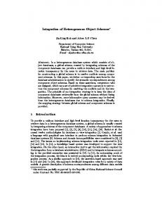
Any contour line of the min and max functions has a sharp corner at the point, where the two arguments have equal value. Following the general approach of [34], we propose to replace the sharp corner in any contour line with a circular arc. Two parabolas, symmetric with respect to the line y = x, are used to delimit the frontier of the circular arc approximation (see Fig. 1 in the case of the smoothed min function). The use of circular approximations for the min and max functions provides the smoothness property of the resulting approximate distance function for constructive shapes built using normal primitives (i.e. defined by Euclidean distance functions). We prevent the radius of the circular arc from growing infinitely by introducing a fixed threshold R. A bounding band is introduced by two parallel straight lines that enclose the arcs with this fixed radius. These band lines are defined by a shift of the line y = x at R distance in positive and negative x directions: y = x – R and y = x + R (see Fig. 1). This bounding band provides a fixed upper limit of the error compared to the min / max approach at any given point.

The two branches of the parabolas are defined to be tangent to the two parallel lines y = x - R and y = x + R at the connecting points (R, 2R) and (2R, R). They are also passing through the origin (0,0); it gives the expressions for these two parabolas: y =

x2 y2 and x = . Note that 4R 4R

the use of parabolas to restrict the circular approximation ensures that the constructed function is C1 in the neighbourhood of the junction between the arc of parabolas and the parallel lines. The resulting defining functions of shapes are built using normal primitives and the newly introduced set-theoretic operations called SARDF operations. The union operation is called SARDF union (we use the symbol “ È S ”) and the intersection operations is called SARDF intersection (with the symbol “ Ç S ”).

Figure 1: The first quadrant is divided into two zones. The growing circular approximation is applied in zone I, whereas we introduce a fixed radius approximation with the bounding band in zone II.

2.3

2.3.1

SARDF intersection of arbitrary objects Construction of the intersection function

The main steps of the construction of the smoothed intersection in the first quadrant (x > 0 and y > 0) are given. By symmetry, the construction in the third quadrant (x < 0 and y < 0) is similar. In the two other quadrants, the expression for the intersection is equal to the min function. Zone I, B Given a point (x, y) in the first quadrant we consider the first case when it is in zone I, B in Fig. 1 and calculate the iso-level value d for the smoothed intersection function at this point. The given point belongs to a circular arc that is tangentially connected to two horizontal and vertical rays when reaching the parabola (see Fig. 1). The equation of this arc is (x - x0)2 + (y - y0)2 = r2, where x0, y0 and r need to be expressed as

where z is the root of (1) verifying z2(2R,R)=R;

functions of the searched value d. The point at the intersection of the parabola and the iso-level d of the searched function, is at a distance d from the axis y = 0. This point belongs also to the parabola, so it x2 y2 satisfies d = 0 , and by symmetry: d = 0 . 4R 4R

The coordinates of the center of the circular arc (x0, y0) satisfy: x0 = y0 = d + r; it follows that r = y0 – d = 2 Rd d. By plugging everything in the equation of the circle, using the substitution of variables d = z and expanding, we obtain the following algebraic equation: z 4 - 4 R z 3 - 4 Rz 2 + 4 R ( x + y ) z - ( x 2 + y 2 ) = 0 (1) Thus in the first quadrant, in the zone I, B, the expression of the intersection is the square of one of the four roots of the algebraic equation (1). The roots of an algebraic equation of degree four are known algebraically. The root of interest is found by using one of the limit conditions, for example d(2R,R) = R. Zone II, inside the bounding band Given a point (x, y) in zone II, within the bounding band (see Fig. 1), the iso-level value d of the smoothed intersection function at that point is searched. This point belongs to a circular arc that is tangentially connected to two horizontal and vertical rays when reaching the two lines of the bounding band. The equation of this circular arc is used: (x - x0)2 + (y - y0)2 = R2. This time R is a constant, only x0 and y0 need to be expressed as functions of d. The coordinates (x0, y0) of the circular arc satisfy: x0 = y0 = d + R. After substitution into the equation of the circular arc and expanding this equation, d comes as one of two solutions of the following algebraic equation of the second degree: 2d 2 + d ( 4 R - 2 x - 2 y ) + 2

2

2

( x + y - 2 R( x + y) + R ) = 0

·

if E1 and f 2 £

f12 , f1 Ç S f 2 = f 2 4R

·

if E1 and f1 £

f 22 , f1 Ç S f 2 = f1 4R

·

if

and

Case 1: f1 > 0 and f2 > 0 In the current paragraph, E1 is used for the following boolean expression: E1 = (f1 < R or f2 < R or (f1 < 2R and f2 < 2R and (f1 – 2R)2 + (f2 – 2R)2 > R2)). ·

If E1 and f 2 >

f12 f2 and f1 > 2 , f1 Ç S f 2 = z 2 , 4R 4R


-R or (f1 > -2R and f2 > -2R and (f1 + R)2 + (f2 + R)2 < R2)). ·

if E2 and f 2 < where

f12 f2 and f1 < - 2 , f1 Ç S f 2 = z , 4R 4R

z

is

the

root

of

d4

d3 1 2 + d ( f1 + f 2 - 2 R) + ( f12 + f 22 ) = 0 2 2R 2R 16 R

verifying z(-2R,-R)=-2R; ·

if E2 and f 2 ³ -

f12 , f1 Ç S f 2 = f 2 4R

·

if E2 and f1 ³ -

f 22 , f1 Ç S f 2 = f1 4R

·

if

Ø

E2

and

f1-R