Constructive Induction for Classifying Time Series

Constructive Induction for Classifying Time Series Mohammed Waleed Kadous1 and Claude Sammut1 University of New South Wales, Sydney, Australia {waleed, claude}@cse.unsw.edu.au

Abstract. We present a method of constructive induction aimed at learning tasks involving multivariate time series data. Using metafeatures, the scope of attribute-value learning is expanded to domains that contain instances that have some kind of recurring substructure, such as strokes in handwriting recognition, or local maxima in time series data. These substructures are used to construct attributes. Metafeatures are applied to two real-world domains: sign language recognition and ECG classification. Using a very generic set of metafeatures we are able to generate classifiers that are either comprehensible or accurate, producing results that are comparable to hand-crafted preprocessing and comparable to human experts. Keywords: machine learning, constructive induction, time series

1

Introduction

There are many domains that do not easily fit into the static attribute-value model so common in machine learning. These include multivariate time series, optical character recognition, sequence recognition, basket analysis and web logs. Consequently, researchers hoping to use attribute-value learners on these domains have few choices: apply hand-crafted preprocessing, write a learner specifically designed for the domain, or use a learner with a more powerful representation, such as relational learning or graph-based induction. Each of these has problems. Hand-crafted preprocessing is frequently used, but requires extensive domain knowledge and concept descriptions are sometimes unnatural. Writing a custom learner is possible, but is labour-intensive. Relational learning techniques tend to be very sensitive to noise and to the particular clausal representation selected. They are typically unable to process large data sets in a reasonable time frame, and/or require the user to set limits on the search such as refinement rules [3]. Furthermore, their most powerful feature – the use of relations – is sometimes not used. In this paper, we use a generic constructive induction technique to allow for domains where instances exhibit recurring substructures. The user defines the recurring substructures, but subsequent steps are automated. Further, the substructures are reusable across domains. These substructures are extracted, and a novel clustering algorithm is used to construct synthetic attributes based on the presence or absence of certain substructures. Standard learners can then be applied.

Learnt concepts are expressed using the same substructures identified by the user. Since these substructures are frequently the same concepts humans use themselves in classifying instances, this results in very readable descriptions. We begin with an overview of applying metafeatures. Experimental results are presented, and we review related work. Finally, we conclude and make some suggestions for future work.

2

Overview

To explain the application of metafeatures, we present a simple pedagogical domain. SoftCorp develops and supports software. Help desk calls are recorded for later analysis. SoftCorp wants to find the critical difference between happy and angry customers. An engineer suggests that the volume level indicates frustration. Each call is therefore divided into 30-second segments; and the average volume in each segment is calculated. If it is high volume, it is marked as “H”, while if it is at a reasonable volume, it is labelled as “L”. On a subset of their data, they determine the outcome by independent means. These are shown in Table 1. Call Loudness (over time) 0 1 0 1 2 3 4 5 6 7 8 9 0 1 L L L H H H L L L L L 2 L L L H L L H L L H H 3 L L H L L H L L L L L 4 L L L L H H H H L L L 5 L L L H H H L L L L 6 L L H H L L H L L H H

Observed events 1 L H L L

Class

2 3 4

{(3, 3)} H {(3, 1), (6, 1), (9, 4)} H H H {(2, 1), (5, 1), (12, 3)} L {(4, 4)} {(3, 3)} H {(2, 2), (6, 1), (9, 3)}

Happy Angry Angry Happy Happy Angry

Table 1. The training set for the Tech Support domain, showing observed LoudRun events.

One expert advises that “runs” of high volume conversation – continuous periods where the conversation runs at a high volume level – are important for classification. Runs of loud volume could be represented as a tuple (t, d) where t is the time at which the conversation becomes loud and d and how long it remains loud. This is an example of a metafeature, called LoudRun. Each instance can now be characterised as having a set of LoudRun events – the LoudRun events are the recurrent substructures appropriate for this domain. These can be extracted by looking for sequences of high-volume conversation. For example, call 2 has one run of highs starting at time 3 lasting for 1 timestep, a high run starting at time 6 lasting for one timestep and a high run starting at time 9 for 4 timesteps. Hence the set of LoudRuns produced from call 2 is {(3, 1), (6, 1), (9, 4)}. To take advantage of attribute-value learners, these sets must be converted into propositional form. A good hypothesis language for such domains consists of rules that check for combinations of particular kinds of events that are critical for classification. For example, in the sign language domain, an upwards motion early in the sign and a movement of the hand forward later in the sign without a

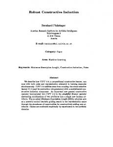
closed hand means thank. Thus we break the learning into two stages: the first to pick out the prototypical instances of an event – in this case: the upwards motion, the movement of the hand forward and the closed hand; and the second to create rules using the prototypical instances. To accomplish the first task, we use a clustering technique similar to instance-based learning, and for the second we use an attribute-value learner. To complete the first stage, the events extracted above can be plotted in the two-dimensional space shown in Figure 1. This is the parameter space. This two-dimensional space consists of one axis for the start time and another for the duration. 5

Angry Happy Synth events

4

Duration (d)

C A

3

2 B

1

0 0

2

4

6 8 Start time (t)

10

12

14

Fig. 1. Paramater space and synthetic events around them for LoudRuns in the Tech Support domain.

Once the points are in parameter space, “typical examples” of LoudRuns can be selected. In this case, the points labelled A, B and C have been selected, as shown in Figure 1. These are termed synthetic events. They may or may not be the same as an observed event – so for example, point A actually corresponds to a real event (the event (3,3) was observed in the data), whereas B and C do not. These synthetic events can be used to segment the parameter space into different regions by computing the Voronoi tiling: for each point in the parameter space, the nearest synthetic event is found. The set of points associated with each synthetic event form a region and the boundaries of each region are calculated. These are shown as dotted lines in Figure 1. To accomplish the second stage, each region constructed in the first stage is used as a test: if a training instance has an event in a region, it “passes” the test. Each training instance is labelled with the test results, each test result effectively becomes an attribute. In this case, three tests A, B and C are constructed and the results shown in Table 2. To construct this table, the “observed events” in Table 2 are examined, and for each region if there is an event that lies within it, a synthetic attribute corresponding to the point is marked as a “yes”.

As a result of the clustering stages above, the initial time series has been converted into a table suitable for learning. In fact, if C4.5 is run on it, the simple tree in Figure 2 results. Stream Class Synth Attrib A B C 1 Happy Yes Yes No 2 Angry No Yes Yes 3 Angry No Yes Yes 4 Happy Yes Yes No 5 Happy Yes Yes No 6 Angry Yes Yes Yes

Table 2. Attribution of synthetic attributes for the Tech Support domain. rgnC = yes: Angry (3.0) rgnC = no: Happy (3.0) Fig. 2. Rule for telling happy and angry customers apart.

This tree says that if the training instance has an event that lies within in region C (i.e. a run of high values that starts around time t=10 and goes for approximately 3.33 timesteps), then its class is Angry. In other words, as long as there is not a long high-volume run towards the end of the conversation, the customer is likely to be happy.

3

Detailed Description

While the idea of metafeatures is simple, there are several possible enhancements and features that need to be considered when implementing a practical system. The TClass algorithm is shown in Table 3. Explanation of each of the components follows. 3.1

Inputs

The input is specified as a set of streams Strain . Each stream represents a single training instance; for example, a single sign. We are also given class labels. The temporal characteristics are represented by a list of time series. Each time series is called a channel. While the Tech Support domain has a single channel (the volume level); the Auslan domain, for example has 22 channels representing various hand position and orientation measures. In addition to temporal characteristics, many domains have non-temporal attributes that are important for classification. For example, when diagnosing ECGs, age, height, weight and gender are important. TClass allows the integration of these conventional features. It is also useful in temporal classification tasks to examine aggregate values of signals and use them as propositional attributes. For example, for continuous

Inputs: Strain = [s1 , ..., sn ] /* Training streams */ Gtrain = [g1 , ..., gn ] /* Specified global attributes */ Ltrain = [l1 , ..., ln ] /* Class labels of training streams */ f = [f1 , ..., fm ] /* Metafeature extraction functions */ w = [w1 , ..., wp ] /* Global attribute calculators */ Outputs: E = [e1 , e2 , ..., em ] /* Synthetic events (each is a set) */ dP /* Learnt classifier */ h /* Human-readable description of learnt concept */ Temporary: Otrain = [o11 , ..., onm ] /* Observed events*/ Atrain = [a1 , ..., an ] /* Global attribute calculator results */ Itrain = [i1 , ..., in ] /* Synthetic attributes */ Btrain = [b1 , ..., bn ] /* All attributes combined */ procedure Train Otrain := ExtractObservedEvents(Strain , f ) E := SelectSyntheticEvents(Otrain , Ltrain ) I := EvaluateSyntheticAttributes(Otrain , E) A := CalculateGlobalAttributes(Strain , w) Btrain := CombineAttributes(Itrain , Atrain , Gtrain ) dP := Learn(Btrain , L) h := ProduceComprehensibleDescription(dP , E, Otrain ) End Table 3. TClass training algorithm

channels, the global maximum and minimum value of a channel, or the mean of each channel may be important attributes. These are termed aggregate global attributes – they measure some property of each training instance as a whole, rather than looking at the temporal structure. To support the use of such aggregate features, TClass supports the use of global attribute calculators. In TClass the global attribute calculators are provided a vector of functions, each function acting on each training stream. Metafeatures form the most critical component of TClass. The formal definition of a metafeature is very simple. It consists of: – A tuple of parameters p = (p1 , ..., pk ), which represents a particular event. Let Pi represent the set of possible values of the parameter pi . Let P be the space of possible parameter values, i.e. P = P1 × P2 × ... × Pk . P is termed the parameter space. – An extraction function f : S → P(P ) which takes a stream s and returns a set of observed events from P . Metafeatures capture a type of recurring temporal substructure, which can then be used as the basis of constructing a propositional feature learner. This work uses a generic set of metafeatures, that are hopefully useful in diverse temporal domains. The metafeatures used are Increasing and Decreasing with the

parameter space (time, average, gradient, duration); Plateau with the parameter space (time, average, duration); and LocalMax and LocalMin which detect local maxima and minima on a single channel (time, value). Additional metafeatures can be easily implemented. 3.2

Processing

Once the metafeatures have been selected, the extraction of observed events is accomplished by applying each metafeature to each training instance. For each metafeature and training instance, a list of the observed events is stored for the the later synthetic event selection. It is also retained for use in attribution. Now that a list of all observed events has been constructed, the synthetic events must be selected. The key insight to selecting these synthetic events is that the distribution of observed events in the parameter space is probably not uniform. An initial approach might be to use standard clustering algorithms, such as K-Means, in the parameter space, i.e., clustering that groups points in such a way that the distance between points within the same cluster is small, and distances between points in different clusters is large. However, this is merely one approach to answering the real question: “Which are the observed events whose presence or absence indicate that the instances belong to a particular class?” The clustering approach can certainly be used to answer this question – the theory being that the different clusters represent different types of observed events. This is an example of unsupervised segmentation. Another approach is to re-pose the question as: “Are there regions in the parameter space where the class distribution is significantly different to what is statistically expected?” This question is very similar to typical problems of supervised classification. This is an example of supervised segmentation: segmentation directed towards creating good features for learning by explicitly considering the class from which an observed event originated. This suggests a more refined approach. Let the set of all observed events be O. Let the set of points we select be E = {e1 , e2 , ..., ek }, where there are k points selected. Define the set of regions R = {R1 , ..., Rk } as: Ri = {x ∈ P |closest(x, E) = ei } and closest(x, E) = argmin dist (x, e) e∈E

where dist is the distance metric we are using for the parameter space. In other words, each region Ri is defined as the set of points in the parameter space P for which ei is the closest point (using the distance metric dist) in the set E. This is the definition of a Voronoi diagram. If the distribution of observed events in a region differs significantly from the global class distribution, then this would be a good feature for classification. Asking whether a training stream has an observed event within a region would be informative of the class of the training stream that the observed event came from.

Measuring the disparity between global and local distributions is well studied in both machine learning and statistics [19]. We will term this measure the disparity measure. Typical disparity measures include χ2 tests, information gain, gain ratio and Gini coefficients. Our objective is to find E such that: R = argmax DispMeas(E) E∈P(O)

In other words, we are looking to find the subset of O (the set of all observed events), E, for which the disparity measure is the greatest. The search, however, is difficult. Hence a “random search” can be employed to solve the problem. While it may first seem that using a random search algorithm is not productive, work by Ho [6] in the field of ordinal optimisation shows that random search is an effective means of finding near-optimal solution. This was also used by Srinivasan [18] in his Aleph ILP system where it was shown to perform well even compared to complex search methods. The random search algorithm is incredibly simple; it picks random subsets of O with an upper bound on the size (in this work we allow subsets with up to ten elements), evaluates the disparity measure on this subset, and if it is the greatest disparity seen so far, it saves the subset. This is repeated for a fixed number of iterations (in this paper, 10,000 iterations are made). The best subset is returned as the set E. We now have a set of synthetic events for each metafeature. Each synthetic event from each metafeature is converted into a synthetic attribute. Each attribute is a test based on whether a given training instance has an observed event that lies within the region around that particular synthetic event. In Table 2, the attributes generated are binary – i.e., we are checking for the presence of particular events. However, this allows only simple decision boundaries. By using the measure D = log2 ( dd21 ), where d1 is the distance to the nearest centroid and d2 is the distance to the second nearest centroid, the backend learner itself can choose the cutpoint and hence decision boundaries can have a more complex shape. This measure has useful properties; for instance, a point on the boundary between two regions has D = 0, whereas the centroid has a measure of D = ∞. This expands the hypothesis language significantly and makes the classification more robust. Attributes are then combined for each instance from the three sources: synthetic attributes, specified global attributes, and calculated global attributes. With this in place, an attribute-value learner can be applied. TClass can use any learner provided by Weka [21]. Both bagging [2] and boosting [16] can also be used. There is a further possibility resulting from the random nature of the synthetic event selection algorithm. Each time the synthetic event selection algorithm runs, it results in a different set of synthetic attributes. Multiple runs of synthetic event selection and the subsequent evaluation and learning stages can be used to create a stochastic ensemble, resulting in improved accuracy, but at the cost of reduced incomprehensibility. Finally, if the learner used at the backend produces descriptions of the form rgnC = yes, then these can be used to create comprehensible descriptions by

Does have a Loud run starting between time 9 and 12 AND lasting between 3 and 4 timesteps: Angry (3.0) Otherwise: Happy (3.0) Fig. 3. Comprehensible description generated from learnt concept

substituting the synthetic event in place of the attribute name. Hence Figure 2 can be converted into Figure 3. The bounds on these values are obtained by drawing a bounding box in the original parameter space of all the instances belonging to region C. Looking at Figure 1, we see that all the points in region C lie within the bounding box d = [3, 4], t = [9, 12]. Note that this is not the same concept that the classifier uses on unseen instances, but it is still useful as an approximation. An obvious modification of this approach allows it to be used with relative membership. 3.3

Testing

Inputs: Stest = [s1 , ..., sn ] /* Test streams */ Gtest = [g1 , ..., gn ] /* Specified global attributes */ f = [f1 , ..., fm ] /* Metafeature extraction functions */ w = [w1 , ..., wp ] /* Global attribute calculators */ E = [e1 , e2 , ..., ek ] /* Synthetic events from training */ dP /* Learnt classifier from training */ Outputs: Ltest = [l1 , ..., ln ] /* Test set labels */ Temporary: Otest = [o11 , ..., onm ] /* Observed events */ Atest = [a1 , ..., an ] /* Global attribute calculated */ Itest = [i1 , ..., in ] /* Synthetic attributes */ Btest = [b1 , ..., bn ] /* Combination of all attributes from all sources */ procedure Test Otest := ExtractObservedEvents(Stest , f ) I := EvaluateSyntheticAttributes(Otest , E) A := ExtractGlobalAttributes(Stest , w) Btest := CombineAttributes(Itest , Atest , Gtest ) Ltest := Classify(Btest , dP ) End Table 4. TClass testing algorithm

The testing algorithm employed by TClass is shown in Table 4. As can be seen it reuses many of the same components used from training. Note that the global attribute calculators and metafeature extraction functions must be the same for both training and testing.

As before, the observed events are extracted, but the synthetic events selected in the training stage are used to create the synthetic attributes. Once the attributes are combined, the classifier built in the training stage can be employed to give a classification.

4

Experiments

We tested TClass on a number of domains. Only brief descriptions are included here; more information can be found in [8]. – The cylinder-bell-funnel (CBF) domain. This domain, proposed by [15], has a single channel and three classes. – A new artificial domain, called TTest, which we created to overcome the limitations of the CBF domain. – Auslan sign recognition: Auslan is the language of the Australian Deaf community. 95 signs were selected and recorded from a native Auslan signer using instrumented gloves. This data has a total of 22 channels covering both hands’ position, orientation and finger bends. – ECG classification: Electrocardigraphs of patients who were healthy or suffered from one of six ailments such as acute myocardial infarctions were recorded. The data has 15 channels in all. The data has a skewed class distribution; with the most common class having approximately 8 times as many examples as the least common class. For comparison, we also applied two baseline learners: – A “naive segmentation” approach, where each channel was subdivided into a certain number of intervals and the mean for each interval computed. This was then fed to a learner. The number of intervals tested were 3, 5, 10, 20. The best results are shown in the table. – Hidden Markov models were applied using Entropic’s HTK [22]. A number of different transition models were considered, such as ergodic, left-right, left-right with one skip. 3,4 and 5-state HMMs were tested. The best results are shown in the table. For the back-end learning, the following learners were used from the Weka package [21]: J48, PART, and bagging and boosting using J48 as the base learner. Also, voting of the boosted learner was performed, using 11 runs of synthetic event construction. The error rates are shown in Table 5. It shows the mean error (percentage) for ten-fold1 cross-validation and the standard error of the mean. The first five use metafeatures, and the last two are baseline learners. The stochastic ensemble employed AdaBoost as the base learner. The χ2 disparity measure was used for supervised segmentation. The results in Table 5 are very promising, although there are some qualifications. Firstly, in every domain, TClass performs as well or better than other 1

For consistency with previous results, 5-fold cross validation was used for the Auslan domain.

Alg J48 PART Bag AB Stochastic Ensemble Naive HMM

CBF 2.3 ± 0.7 4.6 ± 0.8 1.9 ± 0.5 1.4 ± 0.3 0±0 0±0 0±0

TTest 3.3 ± 0.9 2.3 ± 0.3 2.5 ± 0.4 1.0 ± 0.3 0.5 ± 0.2 7.2 ± 0.7 4.4 ± 0.5

Auslan 14.5 ± 0.4 16.7 ± 0.9 9.4 ± 0.8 6.4 ± 0.4 2.1 ± 0.2 5.5 ± 0.5 12.9 ± 0.6

ECG 45.5 ± 1.7 41.9 ± 2.1 35.1 ± 2.6 32.9 ± 2.4 28.2 ± 1.8 28.5 ± 2.6 33.5 ± 1.7

Table 5. Error rates on TClass domain.

learners and the baseline learners – the Auslan and TTest domains are significantly better at the 99.5 per cent level2 . The stochastic ensemble is significantly better than any other TClass method in two of the domains. However, such solutions are less readable, hence forcing a tradeoff between readability and accuracy. The results for Auslan converge with 9 voters, and 11 voters for TTest. The results on the ECG data are worthy of particular note, since de Chazal [4] obtained an error of 28.6% ± 2.4 by hand-crafting an attribute set for a neural network. Given that we were using generic metafeatures and not making use domain knowledge, this result is surprising and promising – since we obtained similar accuracy results (28.2% ± 1.8). Furthermore, in a survey completed by Willems [20], he found that on the same dataset a median human cardiologist obtained an error of 29.7% – less accurate than our system. We were also surprised by the success of the naive approach – almost as accurate as TClass on this domain. We do not understand why it performs so well, and we plan to explore this in future work. As for comprehensibility, for the Auslan domain, definitions generated by TClass compared favourably to the definitions found in the Auslan dictionary [7]. Furthermore, ruleset sizes were reasonable for the Auslan domain of 1.14 rules per class using PART. In the ECG domain, a simple set of 24 rules was found that obtained 40.5 per cent error. Some of these rules showed close correlations with the rules used by existing expert systems [17]. With the TTest domain, it was able to reconstruct the generating concept exactly at low to medium noise levels. In general, in domains with many classes (such as Auslan), it was found that binarizing the learning problem led to more comprehensible definitions than trying to understand complex rules that cover all 95 possible classes.

5

Related Work

This work closely relates to the areas of feature extraction and construction [11], although the formal definitions of extraction and construction assume attributevector representation [11, p. 4]. Liu and Motoda do point to automated preprocessing (or data categorization) as future work [11, p. 9]. They also point to the importance of comprehensibility. It also closely relates to Michalski’s work [12] on constructive induction, but again the work assumes that examples are described in attribute-value format. 2

All significance statements are made using a paired t-test.

There are some general techniques that can be applied to temporal and structured domains. The best developed technique for temporal classification is the hidden Markov model [13]. However, they do suffer some serious drawbacks for general use. Firstly, the structure of the HMM – similar to that of a finite state machine – needs to be specified a priori. Secondly, extracting comprehensible rules from HMMs is not at all easy. Thirdly, there are frequently hundreds or thousands of parameters per HMM. As a result, many training instances are required to learn effectively. Recurrent neural networks and Kohonen maps have also been used to solve temporal and sequence domains [1], but suffer similar problems. Keogh and Pazzani [9] have worked on improving and extending dynamic time warping to temporal domains by representing the time series hierarchically. Lee and Kim [10] take a syntactic approach to time series recognition. Based on knowledge of the financial markets, they develop a grammar for events. Recent interest has also arisen in applying ILP to temporal classification problems. [14] is an interesting example of this, using a tailored search algorithm designed to cope with temporal constraints, although the scalability of this approach is an issue. [5] also presents a system that uses ILP for temporal classification.

6

Conclusions and Future Work

Metafeatures have been applied to diverse domains that exhibit difficult properties: it has been tested on domains with up to 22 channels, 110 metafeatures, 200 megabytes of data, 95 classes, and highly skewed class distributions. They have been shown capable of producing high-accuracy classifiers; in fact, classifiers that match hand-crafted preprocessing techniques. Although the user must define the metafeatures, we have shown that a generic family of metafeatures work for temporal domains. Furthermore, they produce comprehensible descriptions. However, results show that the best accuracy results are achieved using techniques that produce less comprehensible descriptions. This suggests one avenue for future work. The marked difference between the stochastic ensemble and other results points to the weakness of the random search for a good segmentation. For those interested in TClass, it is available at: http://www.cse.unsw.edu.au/~waleed/tclass/

References 1. Yoshua Bengio. Neural Networks for Speech and Sequence Recognition. International Thomson Publishing Inc., 1996. 2. Leo Breiman. Bagging predictors. Machine Learning, 24:123–140, 1996. 3. W. W. Cohen. Learning to classify English text with ILP methods. In L. De Raedt, editor, Proceedings of the 5th International Workshop on Inductive Logic Programming, pages 3–24. Department of Computer Science, Katholieke Universiteit Leuven, 1995. 4. Philip de Chazal. Automatic Classification of the Frank Lead Electrocardiogram. PhD thesis, University of New South Wales, 1998.

5. Pierre Geurts. Pattern extraction for time series classification. In Luc de Raadt and Arno Sieves, editors, Principles of Data Mining and Knowledge Discovery, 5th European Conference, PKDD 2001, Freiburg, Germany, September 3-5, 2001, Proceedings, Lecture Notes in Computer Science. Springer-Verlag, 2001. 6. Y. C. Ho, R. S. Sreenivas, and P. Vakili. Ordinal optimization of DEDS. Discrete Event Dynamic Systems: Theory and Applications, 2(1):61–88, 1992. 7. Trevor Johnston. Auslan Dictionary: a Dictionary of the Sign Language of the Australian Deaf Community. Deafness Resources Australia Ltd, 1989. 8. Mohammed Waleed Kadous. Temporal Classification: Extending the Classification Paradigm to Multivariate Time Series. PhD thesis, School of Computer Science and Engineering, University of New South Wales, 2002. Awaiting review. 9. Eamonn Keogh and Michael Pazzani. Dynamic time warping with higher order features. In SIAM International Conference on Data Mining, SDM 2001. SIAM, 2001. 10. Jae Kyu Lee and Hyun Soon Kim. Intelligent Systems for Finance and Business, chapter 13. John Wiley and Sons Ltd, 1995. 11. Huan Liu and Hiroshi Motoda, editors. Feature Extraction, Construction and Selection: A Data Mining Perspective. Kluwer Academic Publishers, 1998. 12. R. S. Michalski. Machine Learning: An Artificial Intelligence Approach, chapter A Theory and Methodology of Inductive Learning. Tioga Publishers, 1983. 13. Lawrence R. Rabiner. A tutorial on hidden markov models and selected applications in speech recognition. Proceedings of the IEEE, 77(2):257–286, February 1989. 14. Juan J. Rodr´ıguez, Carlos J. Alonso, and Henrik Bostr¨ om. Learning first order logic time series classifiers. In J. Cussens and A. Frisch, editors, Proceedings of ILP2000, pages 260–275, 2000. 15. Naoki Saito. Local feature extraction and its application using a library of bases. PhD thesis, Yale University, December 1994. 16. Robert E. Schapire. A brief introduction to boosting. In Proceedings of the Sixteenth International Joint Conference on Artificial Intelligence, 1999. 17. Schiller Medical. The Schiller ECG Measurement and Interpretation Programs Physicians Guide, 1997. 18. Ashwin Srinivarsan. The Aleph manual. Technical report, Oxford University, 2000. 19. Allan P. White and Wei Zhong Liu. Bias in information-based measures in decision tree induction. Machine Learning, 15:321–329, 1994. 20. J. L. Willems, C. Abreu-Lima, P. Arnaud, C.R. Brohet, and B. Denic. Evaluation of ECG interpretation results obtained by computer and cardiologists. Methods of Information in Medicine, 29(4):pp. 308–316, 1990. 21. Ian H. Witten and Eibe Frank. Data Mining: Practical Machine Learning Tools and Techniques with Java Implementations. Morgan Kaufmann, 1999. 22. Steve Young, Dan Kershaw, Julian Odell, Dave Ollason, Valtcho Valtchev, and Phil Woodland. The HTK Book. Microsoft Corporation, 1998.