Content Based Image Retrieval Using Multiscale Top Points

Content Based Image Retrieval Using Multiscale Top Points A Feasibility Study Frans Kanters, Bram Platel, Luc Florack, and Bart M. ter Haar Romeny Eindhoven University of Technology Den Dolech 2, Postbus 513 5600 MB Eindhoven, The Netherlands {F.M.W.Kanters,B.Platel,L.M.J.Florack,B.M.terHaarRomeny}@tue.nl http://www.bmi2.bmt.tue.nl/image-analysis/

Abstract. A feasibility study for a new method for content based image retrieval is presented. First, an image representation using multiscale top points is introduced. This representation is validated using a minimal variance reconstruction algorithm. The image retrieval problem can now be translated into comparing distances between point sets. For this purpose the proportional transportation distance (PTD) is used. A method is proposed using multiscale top points and their reconstruction coefficients in the PTD to define these distances between images. We present some experiments with promising results on a database with face images.

1

Introduction

In this paper a feasibility study is presented for using multiscale top points in a content based image retrieval system. The goal of such a system is to find, given an image, the closest matches to that image in a large image database, looking at the image content. Many of such systems exist but IBM’s Query by Image Content (QBIC)[12] is probably the best-known one. The user has to specify a number of parameters prior to the searching, so much labor is still needed here. Some examples of more automated systems are Virage [4] and VisualSeek [17] which are based on texture and material structure. Color histogram based systems are also commonly used [18,19]. These systems, however, do not take into account the spatial distribution of the features used. Some examples of systems which do use spatial information are systems which use segmented image regions [11,1]. In the following sections we propose a completely new approach based on an image representation using multiscale top points.

2 2.1

Image Representation Using Multiscale Top Points Introduction

Sometimes it is useful to represent an image in a different way than by it’s pixel values. A “good” representation should contain all the information desired for L.D. Griffin and M. Lillholm (Eds.): Scale-Space 2003, LNCS 2695, pp. 33–43, 2003. c Springer-Verlag Berlin Heidelberg 2003


34

Frans Kanters et al.

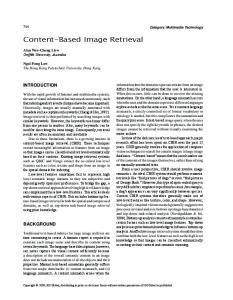
Fig. 1. Simple example top points. Left: original image, right: 3D view of critical paths and top points.

the application and can thus be different for each application. In this chapter we propose an image representation using multiscale top points and some local derivatives in those points. We will verify if the representation contains information about the original image by making a reconstruction from only these top points and some of their local N-jet properties. 2.2

Critical Points, Critical Paths and Top Points

In the Gaussian scale space of a 2D image, a number of points with special differential characteristics can be found [3,2,10,6,9]. In this paper we define the following points: Definition 1. Spatial critical points are points where the spatial gradient is zero. For 2D images these points are maxima, minima or saddles. Definition 2. Critical paths are the paths that spatial critical points follow in scale. Definition 3. Top points are critical points where the Hessian degenerates (det H=0). For generic 2D images, these points are annihilations or creations of saddles with maxima or minima. where the Hessian of a 2D image f is given by:
2 ∂x f Hf =
T
f = ∂y ∂x f

∂x ∂y f ∂y2 f

 (1)

Figure 1 shows a simple image with the critical paths and top points. Note that according to Loog et al. [10] under certain weak conditions always one critical path from a maximum or minimum will be left at the highest scale. In 1D, the top points form a good representation of the signal according to [5]. However, in 2D it is still not proven that using top points results in a good representation of an image. In the next section we will try to reconstruct the original image using it’s top points and the local N-jet properties of the image at those points.

Content Based Image Retrieval Using Multiscale Top Points

2.3

35

Minimal Variance Reconstructions from Multi Scale Points

We present a reconstruction algorithm that preserves top points in the reconstruction and is as smooth as possible. It is based on the minimal variance reconstruction algorithm by Nielsen and Lillholm [13]. We have two constraints: the reconstruction must have the same local N-jet properties at the top points and the variance must be minimal. A quadratic functional is chosen for simplicity of implementation. When using sufficiently many constraints the precise form of the functional does not significantly influence the reconstruction. More information about the reconstruction algorithm can be found in [7]. Given a set of filters φi we thus have to minimize: def S[fˆ] =

 1 ˆ 2 λi f − fˆ | φi  || f ||L2 + 2 i

(2)

Where  . | .  is an inner product in a real Hilbert space1 . The first part satisfies the minimal variance constraint, the second part makes sure that the features are preserved. Using the functional derivative we obtain: δS[fˆ] def ˆ  λi φi = f− δ fˆ

(3)

i

we can determine the unique solution of fˆ =



δS[fˆ] δ fˆ

= 0:

λi φi

(4)

i

which is the fˆ that minimizes the variance if the coefficients λi are calculated by substitution of (4) in: f − fˆ | φj  = 0 (5) Now we define the following filters: φi,ν1 ...νk (x, y) =

√

k

2ti ∇ν1 ...νk φ(x − xi , y − yi , ti )

(6)

with φ the standard Gaussian at scale t centered at the origin, thus 1 − x2 +y2 e 4t (7) 4πt Using (6) in (4), we obtain our reconstruction formula for top points, using derivatives up to the second order. Note that the summation convention for repeated indices applies for all spatial indices µ = x, y and ρ = x, y. The reconstruction formula becomes: φ(x, y, t) =

fˆ(x, y) =

N  i=1

ai φi (x, y) + bµi φi,µ (x, y) + cµρ i φi,µρ (x, y)

(8)

subject to the constraints: 1

Or bilinear functional on the product space of fiducial filters (containing at least the Gaussian family) and its topological dual (i.e. the raw images).

36

Frans Kanters et al.

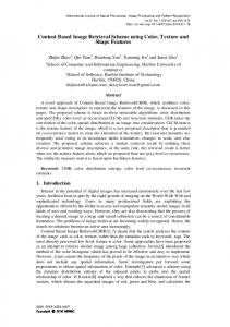
Fig. 2. Reconstruction from top points of mrbrain.tif. Left: original image, Center: 3D view of critical paths and top points, Right: reconstruction from top points, using all features with order k ≤ 2.

 f − fˆ | φi  = 0,  f − fˆ | φi,µ  = 0

and  f − fˆ | φi,µρ  = 0

(9)

xy yy The coefficients ai , bxi , byi , cxx i , ci and ci can be calculated from the constraints using simple linear algebra. Each coefficient determines how much the corresponding derivative of the Gaussian is used for the reconstructed image at point i. Later we will use these coefficients for our image retrieval system. Given a number of (top) points and their local derivatives up to the second order we can make a reconstruction of the image using the reconstruction formula (8). Figure 2 shows the result of a reconstruction using only top points and some local derivatives. Note that the reconstruction is not a perfect one, but for our purpose it is only important to show that the information carried within the top points is sufficiently rich.

3

3.1

Content Based Image Retrieval Using Multiscale Top Points Introduction

In this section we try to use the top point representation for image matching in a database. How much two images “look” alike is now translated into how “close” two point sets are to each other. Of course, a lot of different distance measures can be used here. In each top point we can calculate some properties (e.g. derivatives, reconstruction coefficients) which can be taken into account for the distance. The number of top points will generally be different for each image. For the distance measurement we chose to use the Proportional Transportation Distance (PTD) as introduced by P. Giannopoulos and R. Veltkamp [14], which is based on the Earth Movers Distance (EMD) [20]. The PTD is a pseudo metric which can be used on weighted point sets. The advantage of the PTD lies in the fact that it holds the triangle inequality which can be used to speed up the retrieval process.

Content Based Image Retrieval Using Multiscale Top Points

3.2

37

Proportional Transportation Distance (PTD)

First, we define weighted point sets. Definition 4. Let A = {a1 , a2 , . . . , am } be a weighted point set such that ai = k + (xi , wi ), i = 1, . . . , m, where m xi ∈ R with wi ∈ R ∪ {0} being its corresponding weight. Let also W = i=1 wi be the total weight of set A. Definition 5. Let B = {b1 , b2 , . . . , bn } be a weighted point set such that bj = (xj , uj ), j = 1, . . . , n,  where xj ∈ Rk with uj ∈ R+ ∪ {0} being its corresponding n weight. Let also U = j=1 uj be the total weight of set B. The PTD can then be defined as follows: Definition 6. Let A and B be two weighted point sets and dij a ground distance between point ai and bj . The set of all feasible flows F = [fij ] from A to B, is now defined by the following constraints: (i) f ij ≥ 0, i = 1, . . . , m, j = 1, . . . , n n (ii) fij = wi , i = 1, . . . , m j=1 uj W m (iii) i=1 f ij = U , j = 1, . . . , n m n (iv) i=1 j=1 fij = W then the PTD can be defined as: P T D(A, B) =

minF ∈F

m n i=1

j=1

fij dij

W

The PTD can be seen as the minimum amount of work needed to transform A into a new set A
that resembles B. In particular, we redistribute A’s total weight from the position of its points to the position of B’s points leaving the old percentages of weights in B the same. For calculation of the PTD we used a fast implementation of the Earth Movers Distance (EMD) which is publicly available [20,15]. In our case we used normalized weights such that U = W = 1. There are two major parameters with which we can experiment. The first one is the ground distance dij . All top points have the following properties: xy yy x y xx xy yy pi = (xi , yi , ti , ai , bxi , byi , cxx i , ci , ci ), with ai , bi , bi , ci , ci , ci the reconstruction coefficients of (8). One possible ground distance is the Euclidian distance for only the x and y coordinates, discarding all other features. Another possibility is to include the reconstruction coefficients of each point in the ground distance. The second tuneable parameter is the weight wi for each point. We can use equal weights for all points but we can also use different weights for each point, for example by using the reconstruction coefficients of (8) in the weights. In the next section a number of different settings for these parameters are used for content based image retrieval experiments.

38

4

Frans Kanters et al.

Experimental Results

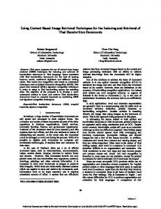
In the previous section we described a method to calculate a distance between two weighted point sets, the PTD. We can use this PTD for content based image retrieval in a large database. In the experiments described in this section, we used a subset of the Face database from the Olivetti Research Laboratory, made by Samaria and Harter [16]. The subset consists of 200 images of faces from 20 people (10 images each, with different deviations such as pose, glasses, distortion). From every image of this set, the top points and the reconstruction coefficients were calculated. For the content based image retrieval experiment we used the first image of each person as a query and looked at the 9 images with the smallest PTD to this image, using different parameters. 4.1

Experiment 1

In our first experiment the ground distance is defined as:  dij = (xi − xj )2 + (yi − yj )2 + (ti − tj )2

(10)

and the weights are equally distributed, thus: 1 m 1 uj = n

wi =

(11) (12)

While the ground distance is obviously ad hoc and the weights do not contain any information, the results are surprising. As can be seen in Fig. 3, the images in the database with the smallest PTD are mostly from the same person. Note that in the second row, the results seem to be independent of the glasses. Also note that the third row is one of the worst query results from the database for this experiment (in this case, the hair line seems to have a strong influence). Somehow, the structure of the faces is more important than the pose of the person for the PTD algorithm. 4.2

Experiment 2

In our second experiment the ground distance is defined as in (10), but the weights are different. Our first try was to take the mean of the absolute values of the reconstruction coefficients (admittedly somewhat an ad hoc choice): xy yy |ai | + |bxi | + |byi | + |cxx i | + |ci | + |ci | 6 xy yy |aj | + |bxj | + |byj | + |cxx j | + |cj | + |cj | uj = 6

wi =

(13) (14)

The results of this first try can be seen in Fig. 4. As can be seen, the results are absolutely not close to the results from the first experiment. It seems

Content Based Image Retrieval Using Multiscale Top Points

39


Fig. 3. Experiment 1: dij = (xi − xj )2 + (yi − yj )2 + (ti − tj )2 and weights are equally distributed. Leftmost images are queries, neighboring images are closest matches, with increasing PTD.

that some points have a much too large weight. Looking at the range of the reconstruction coefficients, the problem becomes more clear. Sometimes the reconstruction coefficients can be as high as 106 , resulting in very strong points, where distance is not very important anymore. As a second try we take the log of the weights from (13):
xy yy  |ai | + |bxi | + |byi | + |cxx i | + |ci | + |ci | (15) wi = log 6   xy yy |aj | + |bxj | + |byj | + |cxx j | + |cj | + |cj | uj = log (16) 6 The results are shown in Fig. 5. The results are much better than with (1314), but still not as good as with equally distributed weights. It is clear that one has to think more carefully about the way in which the incommensurable features are to be incorporated, instead of just averaging the features as in (13-14). 4.3

Experiment 3

For image retrieval, it is desired to be independent of translations and rotations of the query image. When looking at the top point structure of an image, one question is how much information is contained in the position of the top points. As a final experiment we tried a ground distance which is translation invariant, because the x and y coordinates are left out. Here things are becoming mildly interesting. We propose the ground distance as:  µρ 2 dij = (ti − tj )2 + (ai − aj )2 + (bνi − bνj )2 + (cµρ (17) i − cj )

40

Frans Kanters et al.


Fig. 4. Experiment 2a: dij = (xi − xj )2 + (yi − yj )2 + (ti − tj )2 and mean of absolute reconstruction coefficients as weights. Leftmost images are queries, neighboring images are closest matches, with increasing PTD.


Fig. 5. Experiment 2b: dij = (xi − xj )2 + (yi − yj )2 + (ti − tj )2 and Log of mean of absolute reconstruction coefficients as weights. Leftmost images are queries, neighboring images are closest matches, with increasing PTD.

for all spatial indices ν, µ, ρ. The weights are taken the same as in (15). The results for this experiment are shown in Fig. 6. It is very surprising to see that the results are better without the position of the top points in the ground distance. Still there are some queries which give problems, as can be seen in the fourth row of Fig. 6. The big advantage with this ground distance is the invariance regarding translation. Note that for all described methods, some odd results can show up. For example the fifth image on the third row of Fig. 6 appears to be very different

Content Based Image Retrieval Using Multiscale Top Points

41

 µρ 2 Fig. 6. Experiment 3a: dij = (ti − tj )2 + (ai − aj )2 + (bνi − bνj )2 + (cµρ i − cj ) and Log of mean of absolute reconstruction coefficients as weights. Leftmost images are queries, neighboring images are closest matches, with increasing PTD.

from the rest, but for the algorithm it is closer to the query than the sixth image. These results can not be explained at this moment and have to be further investigated.

5

Conclusions and Discussion

In this paper we presented a method for content based image retrieval using a multiscale top points representation of an image. The first experiments on a face database of 200 images are promising, but a lot of further research must be done. There are two main parameters in the PTD that must be further investigated, the ground distance and the weights of the points. In our experiments we made some ad hoc choices for the ground distance. Better results will be possible if other ground distances are used. It is possible to obtain translation, rotation and scale invariance by choosing the correct ground distance. For the weights of the points in the point sets holds the same; we only tested a few rather ad hoc weight values. The importance of a single top point for the reconstruction of the image should be expressed in the weight for that top point. In one test we used the reconstruction coefficients to calculate the weights, but it might be easier to use the local derivatives in the top points instead. With this representation it might also be possible to search for substructures in an image. If for example the top point representation of a face is known, it might be possible to search for a subset of top points in a complete scene of different faces. At this moment, no topological information from the top points is used. However, it is possible to make a graph from the top points which does contain topo-

42

Frans Kanters et al.

logical information. The point matching then becomes graph matching, which is a well known research area. It might be that content based image retrieval using such graphs is more robust than using point sets.

Acknowledgements This work is part of the DSSCV project supported by the IST Programme of the European Union (IST-2001-35443).

References 1. C. Carson, M. Thomas, S. Belongie, J. M. Hellerstein, and J. Malik. Blobworld: A system for region-based image indexing and retrieval. In Third International Conference on Visual Information Systems. Springer, 1999. 2. L. Florack and A. Kuijper. The topological structure of scale-space images. Journal of Mathematical Imaging and Vision, 12(1):65–79, February 2000. 3. L. D. Griffin and A. C. F. Colchester. Superficial and deep structure in linear diffusion scale space: Isophotes, critical points and separatrices. Image and Vision Computing, 13(7):543–557, September 1995. 4. Amarnath Gupta and Ramesh Jain. Visual information retrieval. Communications of the ACM, 40(5):70–79, 1997. 5. P. Johansen, S. Skelboe, K. Grue, and J. D. Andersen. Representing signals by their top points in scale-space. In Proceedings of the 8th International Conference on Pattern Recognition (Paris, France, October 1986), pages 215–217. IEEE Computer Society Press, 1986. 6. S. N. Kalitzin, B. M. ter Haar Romeny, A. H. Salden, P. F. M. Nacken, and M. A. Viergever. Topological numbers and singularities in scalar images: Scalespace evolution properties. Journal of Mathematical Imaging and Vision, 9(3), November 1998. 7. F.M.W. Kanters, L.M.J. Florack, B. Platel and B.M. ter Haar Romeny. Image reconstruction from multiscale critical points. Elsewhere in these proceedings. 8. M. Kerckhove, editor. Scale-Space and Morphology in Computer Vision: Proceedings of the Third International Conference, Scale-Space 2001, Vancouver, Canada, volume 2106 of Lecture Notes in Computer Science. Springer-Verlag, Berlin, July 2001. 9. A. Kuijper and L.M.J. Florack. The application of catastrophe theory to image analysis. Submitted to Image and Vision Computing. 10. M. Loog, J. J. Duistermaat, and L. M. J. Florack. On the behavior of spatial critical points under Gaussian blurring. a folklore theorem and scale-space constraints. In Kerckhove [8], pages 183–192. 11. Wei-Ying Ma and B. S. Manjunath. Netra: A toolbox for navigating large image databases. Multimedia Systems, 7(3):184–198, 1999. 12. M.Flickner, H.Sawhney, et.al. Query by image and video content: the qbic system. IEEE Computer, 28(9):23–32, 1995. 13. M. Nielsen and M. Lillholm. What do features tell about images? In Kerckhove [8], pages 39–50. 14. R. Veltkamp P. Giannopoulos. A pseudo-metric for weighted point sets. In ECCV 2002, LNCS 2352, pages 715–730. Springer, 2002.

Content Based Image Retrieval Using Multiscale Top Points

43

15. Y. Rubner. Code for earth movers distance (emd). http://vision.stanford.edu/˜rubner/emd/default.htm. 16. F. Samaria and A. Harter. Parameterisation of a stochastic model for human face identification, 1994. 17. J. Smith and S. Chang. Single color extraction and image query, 1995. 18. Markus Stricker and Michael Swain. The capacity and the sensitivity of color histogram indexing. Technical Report TR-94-05, University of Chicago, 3 1994. 19. M. Swain and D. Ballard. Color indexing. International Journal on Computer Vision, 7(1):11–32, 1991. 20. L.J. Guibas Y. Rubner, C. Tomasi. A metric for distributions with applications to image databases. In IEEE International Conference on Computer Vision, Bombay, India, pages 59–66, 1998.