Content-based image sequence representation - omni.isr.tecnico

1526_C02.fm Page 5 Monday, May 17, 2004 12:44 PM

chapter 2

Content-based image sequence representation Pedro M. Q. Aguiar, Radu S. Jasinschi, José M. F. Moura, and Charnchai Pluempitiwiriyawej1 Contents 2.1 Introduction ................................................................................................... 7 2.1.1 Mosaics for static 3-D scenes and large depth: single layer ........................................................................................ 9 2.1.2 Mosaics for static 3-D scenes and variable depth: multiple layers ................................................................................. 11 2.1.3 Video representations with fully 3-D models ........................... 11 2.1.3.1 Structure from motion: factorization............................ 12 2.2 Image segmentation .................................................................................. 13 2.2.1 Calculus of variations.................................................................... 13 2.2.1.1 Adding constraints ............................................................ 16 2.2.1.2 Gradient descent flow..................................................... 16 2.2.2 Overview of image segmentation methods............................... 17 2.2.2.1 Edge-based approach...................................................... 18 2.2.2.2 Region-based approach .................................................. 18 2.2.3 Active contour methods................................................................ 19 2.2.4 Parametric active contour ............................................................. 20 2.2.4.1 Variations of classical snakes......................................... 22 2.2.5 Curve evolution theory ................................................................. 24 2.2.6 Level set method ............................................................................ 28 2.2.7 Geometric active contours ............................................................ 30 1

The work of the first author was partially supported by the (Portuguese) Foundation for Science and Technology grant POSI/SRI/41561/2001. The work of the third and fourth authors was partially supported by ONR grant # N000 14-00-1-0593 and by NIH grants R01EB/AI-00318 and P41EB001977. 0-8493-1526-3/2004/$0.00+$1.50 © 2004 by CRC Press LLC

5


6

Digital Image Sequence Processing

2.2.8 STACS: Stochastic active contour scheme.................................. 2.3 Mosaics: From 2-D to 3-D ........................................................................ 2.3.1 Generative video ........................................................................... 2.3.1.1 Figure and background mosaics generation............... 2.3.2 3-D Based mosaics ........................................................................ 2.3.2.1 Structure-from-motion: generalized eight-point algorithm........................................................................... 2.3.2.2 Layered mosaics based on 3-D information ............... 2.3.2.3 3-D mosaics....................................................................... 2.3.2.4 Summary........................................................................... 2.4 Three-dimensional object-based representation .................................... 2.4.1 3-D object modelling from video................................................. 2.4.1.1 Surface-based rank 1 factorization method ................ 2.4.2 Framework ...................................................................................... 2.4.2.1 Image sequence representation ..................................... 2.4.2.2 3-D motion representation ............................................. 2.4.2.3 3-D shape representation................................................ 2.4.3 Video analysis ................................................................................. 2.4.3.1 Image motion ................................................................... 2.4.3.2 3-D structure from 2-D motion ..................................... 2.4.3.3 Translation estimation..................................................... 2.4.3.4 Matrix of 2-D motion parameters................................. 2.4.3.5 Rank 1 factorization ........................................................ 2.4.3.6 Decomposition stage ...................................................... 2.4.3.7 Normalization stage ........................................................ 2.4.3.8 Texture recovery .............................................................. 2.4.4 Video synthesis ............................................................................... 2.4.5 Experiment ...................................................................................... 2.4.6 Applications .................................................................................... 2.4.6.1 Video coding..................................................................... 2.4.6.2 Video content addressing............................................... 2.4.6.3 Virtualized reality ............................................................ 2.4.7 Summary ........................................................................................ 2.5 Conclusion.................................................................................................... References.............................................................................................................. Abstract. In this chapter we overview methods that represent video sequences in terms of their content. These methods differ from those developed for MPEG/H.26X coding standards in that sequences are described in terms of extended images instead of collections of frames. We describe how these extended images, e.g., mosaics, are generated by basically the same principle: the incremental composition of visual photometric, geometric, and multi-view information into one or more extended images. Different outputs, e.g., from single 2-D mosaics to full 3-D mosaics,

32 34 35 35 41 43 45 49 51 52 52 52 53 54 54 55 56 56 57 58 59 60 60 60 61 62 63 64 64 66 67 68 68 68


Chapter 2:

Content-based image sequence representation

7

are obtained depending on the quality and quantity of photometric, geometric, and multi-view information. In particular, we detail a framework well suited to the representation of scenes with independently moving objects. We address the two following important cases: (i) the moving objects can be represented by 2-D silhouettes (generative video approach) or (ii) the camera motion is such that the moving objects must be described by their 3-D shape (recovered through rank 1 surface-based factorization). A basic preprocessing step in content-based image sequence representation is to extract and track the relevant background and foreground objects. This is achieved by 2-D shape segmentation for which there is a wealth of methods and approaches. The chapter includes a brief description of active contour methods for image segmentation.

2.1 Introduction The processing, storage, and transmission of video sequences are now common features of many commercial and free products. In spite of the many advances in the representation of video sequences, especially with the advent and the development of the MPEG/H.26X video coding standards, there is still room for more compact video representations than currently used by these standards. In this chapter we describe work developed in the last 20 years that addresses the problem of content-based video representation. This work can be seen as an evolution from standard computer vision, image processing, computer graphics, and coding theory toward a full 3-D representation of visual information. Major application domains using video sequences information include visually guided robotics, inspection, and surveillance; and visual rendering. In visually guided robotics, partial or full 3-D scene information is necessary, which requires the full reconstruction of 3-D information. On the other hand, inspection and surveillance robotics often requires only 2-D information. In visual rendering, the main goal is to display the video sequence in some device in the best visual quality manner. Common to all these applications is the issue of compact representation since full quality video requires an enormous amount of data, which makes its storage, processing, and transmission a difficult problem. We consider in this paper a hierarchy of content-based approaches: (i) generative video (GV) that generalizes 2-D mosaics; (ii) multilayered GV type representations; and (iii) full 3-D representation of objects. The MPEG/H.26X standards use frame-based information. Frames are represented by their GOP structure (e.g., IPPPBPPPBPPPBPPP), and each frame is given by slices composed of macro-blocks that are made of typically 8 ¥ 8 DCT blocks. In spite of many advances allowed by this representation, it falls short in terms of the level of details represented and compression


8


rates. DCT blocks for spatial luminance/color coding and macro-blocks for motion coding provide the highest levels of details. However, they miss capturing pixel-level luminance/color/texture spatial variations and temporal (velocity) variations, thus leading to visual artifacts. The compression ratios achieved, e.g., 40:1, are still too low for effective use of MPEG/H.26X standards in multimedia applications for storage and communication purposes. Content-based representations go beyond frame-based or pixel-based representations of sequences. Video content information is represented by objects that have to be segmented and represented. These objects can be based on 2-D information (e.g., faces, cars, or trees) or 3-D information (e.g., when faces, cars, or trees are represented in terms of their volumetric content). Just segmenting objects from individual video frames is not sufficient; these segmented objects have to be combined across the sequence to generate extended images for the same object. These extended images, which include mosaics, are an important element in the “next generation” systems for compact video representation. Extended images stand midway between frame-based video representations and full 3-D representations. With extended images, a more compact representation of videos is possible, which allows for their more efficient processing, storage, and transmission. In this chapter we discuss work on extended images as a sequence of approaches that start with standard 2-D panoramas or mosaics, e.g., those used in astronomy for very far objects, to full 3-D mosaics used in visually guided robotics and augmented environments. In the evolution from standard single 2-D mosaics to full 3-D mosaics, more assumptions and information about the 3-D world are used. We present this historical and technical evolution as the development of the same basic concept, i.e., the incremental composition of photometric (luminance/color), shape (depth), and points of view (multiview) information from successive frames in a video sequence to generate one or more mosaics. As we make use of additional assumptions and information about the world, we obtain different types of extended images. One such content-based video representation is called generative video (GV). In this representation, 2-D objects are segmented and compactly represented as, for example, coherent stacks of rectangles. These objects are then used to generate mosaics. GV mosaics are different from standard mosaics. GV mosaics include the static or slowly changing background mosaics, but they also include foreground moving objects, which we call figures. The GV video representation includes the following constructs: (i) layered mosaics, one for each foreground moving 2-D object or objects lying at the same depth level; and (ii) a set of operators that allow for the efficient synthesis of video sequences. Depending on the relative depth between different objects in the scene and the background, a single or a multi-layered representation may be needed. We have shown that GV allows for a very compact video sequence representation, which enables a very efficient coding of videos with compression ratios in the range of 1000:1.


Chapter 2:


9

Often, layered representations are not sufficient to describe well the video sequence, for example, when the camera motion is such that the rigidity of the real-world objects can only be captured by going beyond 2-D shape models and resorting to fully 3-D models to describe the shape of the objects. To recover automatically the 3-D shape of the objects and the 3-D motion of the camera from the 2-D motion of the brightness pattern on the image plane, we describe in this chapter the surface-based rank 1 factorization method. Content-based video representations, either single-layer or multiple-layer GV, or full 3-D object representations involve as an important preprocessing step the segmentation and tracking of 2-D objects. Segmentation is a very difficult problem for which there is a wealth of approaches described in the literature. We discuss in this chapter contour-based methods that are becoming popular. These methods are based on energy minimization approaches and extend beyond the well-known “snakes” method in which a set of points representing positions on the image boundary of 2-D objects — contours — is tracked in time. These methods make certain assumptions regarding the smoothness of these contours and how they evolve over time. These assumptions are at the heart of representing “active” contours. For completeness, we briefly discuss active-contour-based segmentation methods in this chapter. In the next three subsections, we briefly overview work by others on single- and multilayered video representations and 3-D representations. Section 2.2 overviews active-contour-based approaches to segmentation. We then focus in Section 2.3 on generative video and its generalizations to multilayered representations and in Section 2.4 on the rank 1 surface-based 3-D video representations. Section 2.5 concludes the chapter.

2.1.1

Mosaics for static 3-D scenes and large depth: single layer

Image mosaics have received considerable attention from the fields of astronomy, biology, aerial photogrammetry, and image stabilization to video compression, visualization, and virtualized environments, among others. The main assumption in these application domains is that the 3-D scene layout is given by static regions shown very far away from the camera, that is, with large average depth values with respect to (w.r.t.) to the camera (center). Methods using this assumption will be discussed next. Lippman [1] developed the idea of mosaics in the context of video production. This reference deals mostly with generating panoramic images describing static background regions. In this technique, panoramic images are generated by accumulating and integrating local image intensity information. Objects moving in the scene are averaged out; their shape and position in the image are described as a “halo” region containing the background region; the position of the object in the sequence is reconstructed by appropriately matching the background region in the halo to that of the background region in the enlarged image. Lippan’s target application is


10

AU: Who is “they”? Burt


high-definition television (HDTV) systems that require the presentation of video at different aspect ratios compared to standard TV. Burt and Adelson [2] describe a multiresolution technique for image mosaicing. Their aim is to generate photomosaics for which the region of spatial transition between different images (or image parts) is smooth in terms of its gray level or color difference. They use for this purpose Laplacian pyramid structures to decompose each image into their component pass-band images defined at different spatial resolution levels. For each band, they generate a mosaic, and the final mosaic is given by combining the mosaics at the different pass-bands. Their target applications are satellite imagery and computer graphics. Hansen [3, 4] and collaborators at the David Sarnoff Laboratory have developed techniques for generating mosaics in the framework of military reconnaissance, surveillance, and target detection. Their motivation is image stabilization for systems moving at high speeds and that use, among other things, video information. The successive images of these video sequences display little overlap, and they show, in general, a static 3-D scene and in some cases a single moving (target) object. Image or camera stabilization is extremely difficult under these circumstances. Hansen and coworkers use a mosaic-based stabilization technique by which a given image of the video sequence is registered to the mosaic built from preceding images of the sequence instead of just from the immediately preceding image. This mosaic is called the reference mosaic. It describes an extended view of a static 3-D terrain. The sequential mosaic generation is realized through a series of image alignment operations, which include the estimation of global image velocity and of image warping. Teodosio and Bender [5] have proposed salient video stills as a novel way to represent videos. A salient still represents the video sequence by a single high-resolution image by translating, scaling, and warping images of the sequence into a single high-resolution raster. This is realized by (i) calculating the optical flow between successive images; (ii) using an affine representation of the optical flow to appropriately translate, scale, and warp images; and (iii) using a weighted median of the high-resolution image. As an intermediate step, a continuous space–time raster is generated in order to appropriately align all pixels, regardless of whether the camera pans or zooms, thus creating the salient still. Irani et al. [6] propose a video sequence representation in terms of static, dynamic, and multiresolution mosaics. A static mosaic is built from collections of “submosaics,” one for each scene subsequence, by aligning all of its frames to a fixed coordinate system. This type of mosaic can handle cases of static scenes, but it is not adequate for one having temporally varying information. In the later case, a dynamic mosaic is built from a collection of evolving mosaics. Each of these temporarily updated mosaics is updated according to information from the most recent frame. One difference with static mosaic generation is that the coordinate system of the dynamic mosaics can be moving with the current frame. This allows for an efficient updating of the dynamic content.


Chapter 2:


11

2.1.2 Mosaics for static 3-D scenes and variable depth: multiple layers When a camera moves in a static scene containing fixed regions or objects that cluster at different depth levels, it is necessary to generate multiple mosaics, one for each layer. Wang and Adelson [7] describe a method to generate layers of panoramic images from video sequences generated through camera translation with respect to static scenes. They use the information from the induced (camera) motion. They segment the panoramic images into layers according to the motion induced by the camera motion. Video mosaicing is pixel based. It generates panoramic images from static scenery panned or zoomed by a moving camera.

2.1.3

Video representations with fully 3-D models

The mosaicing approaches outlined above represent a video sequence in terms of flat scenarios. Since the planar mosaics do not model the 3-D shape of the objects, these approaches do not provide a clear separation among object shape, motion, and texture. Although several researchers proposed enhancing the mosaics by incorporating depth information (see, for example, the plane + parallax approach [8, 6]), these models often do not provide meaningful representations for the 3-D shape of the objects. In fact, any video sequence obtained by rotating the camera around an object demands a content-based representation that must be fully 3-D based. Among 3-D-model-based video representations, the semantic coding approach assumes that detailed a priori knowledge about the scene is available. An example of semantic coding is the utilization of head and shoulders parametric models to represent facial video sequences (see [9, 10]). The video analysis task estimates along time the small changes of the head-and-shoulders model parameters. The video sequence is represented by the sequence of estimated head-and-shoulders model parameters. This type of representation enables very high compression rates for the facial video sequences but cannot cope with more general videos. The use of 3-D-based representations for videos of general scenes demands the automatic 3-D modeling of the environment. The information source for a number of successful approaches to 3-D modeling has been a range image (see, for example, [11, 12]). This image, obtained from a range sensor, provides the depth between the sensor and the environment facing it on a discrete grid. Since the range image itself contains explicit information about the 3-D structure of the environment, the references cited above deal with the problem of how to combine a number of sets of 3-D points (each set corresponding to a range image) into a 3-D model. When no explicit 3-D information is given, the problem of computing automatically a 3-D-model-based representation is that of building the 3-D


12


models from the 2-D video data. The recovery of the 3-D structure (3-D shape and 3-D motion) of rigid objects from 2-D video sequences has been widely considered by the computer vision community. Methods that infer 3-D shape from a single frame are based on cues such as shading and defocus. These methods fail to give reliable 3-D shape estimates for unconstrained real-world scenes. If no prior knowledge about the scene is available, the cue to estimating the 3-D structure is the 2-D motion of the brightness pattern in the image plane. For this reason, the problem is generally referred to as structure from motion (SFM).

2.1.3.1 Structure from motion: factorization Among the existing approaches to the multiframe SFM problem, the factorization method [13] is an elegant method to recover structure from motion without computing the absolute depth as an intermediate step. The object shape is represented by the 3-D position of a set of feature points. The 2-D projection of each feature point is tracked along the image sequence. The 3-D shape and motion are then estimated by factorizing a measurement matrix whose columns are the 2-D trajectories of each of the feature point projections. The factorization method proved to be effective when processing videos obtained in controlled environments with a relatively small number of feature points. However, to provide dense depth estimates and dense descriptions of the shape, this method usually requires hundreds of features, a situation which then poses a major challenge in tracking these features along the image sequence and that leads to a combinatorially complex correspondence problem. In Section 2.4, we describe a 3-D-model-based video representation scheme that overcomes this problem by using the surface-based rank 1 factorization method [14, 15]. There are two distinguishing features of this approach. First, it is surface based rather than feature (point) based; i.e., it describes the shape of the object by patches, e.g., planar patches or higher-order polynomial patches. Planar patches provide not only localization but also information regarding the orientation of the surface. To obtain similar-quality descriptions of the object, the number of patches needed is usually much smaller than the number of feature points needed. In [14], it is shown that the polynomial description of the patches leads to a parameterization of the object surface and this parametric description of the 3-D shape induces a parametric model for the 2-D motion of the brightness pattern in the image plane. Instead of tracking pointwise features, this method tracks regions of many pixels, where the 2-D image motion of each region is described by a single set of parameters. This approach avoids the correspondence problem and is particularly suited for practical scenarios in which the objects are, for example, large buildings that are well described by piecewise flat surfaces. The second characteristic of the method in [14, 15] and in Section 2.4 is that it requires only the factorization of a rank 1 rather than rank 3 matrix, which simplifies significantly the computational effort of the approach and is more robust to noise.


Chapter 2:


13

Clearly, the generation of images from 3-D models of the world is a subject that has been addressed by the computer graphics community. When the world models are inferred from photograph or video images, rather than specified by an operator, the view generation process is known as image based rendering (IBR). Some systems use a set of calibrated cameras (i.e., with known 3-D positions and internal parameters) to capture the 3-D shape of the scene and synthesize arbitrary views by texture mapping, e.g., the Virtualized Reality system [16]. Other systems are tailored to the modeling of specific 3-D objects like the Façade system [17], which does not need a priori calibration but requires user interaction to establish point correspondences. These systems, as well as the framework described in Section 2.4, represent a scene by using geometric models of the 3-D objects. A distinct approach to IBR uses the plenoptic function [18]—an array that contains the light intensity as a function of the viewing point position in 3-D space, the direction of propagation, the time, and the wavelength. If in empty space, the dependence on the viewing point position along the direction of propagation may be dropped. By dropping also the dependence on time, which assumes that the lighting conditions are fixed, researchers have attempted to infer from images what has been called the light field [19]. A major problem in rendering images from acquired light fields is that, due to limitations on the number of images available and on the processing time, they are usually subsampled. The Lumigraph system [20] overcomes this limitation by using the approximate geometry of the 3-D scene to aid the interpolation of the light field.

2.2 Image segmentation In this section, we discuss segmentation algorithms, in particular, energy minimization and active-contour-based approaches, which are popularly used in video image processing. In Subsection 2.2.1, we review concepts from variational calculus and present several forms of the Euler-Lagrange equation. In Subsection 2.2.2, we broadly classify the image segmentation algorithms into two categories: edge-based and region-based. In Subsection 2.2.3, we consider active contour methods for image segmentation and discuss their advantages and disadvantages. The seminal work on active contours by Kass, Witkin, and Terzopoulos [21], including its variations, is then discussed in subsection 2.2.4. Next, we provide in Subsection 2.2.5 background on curve evolution, while Subsection 2.2.6 shows how curve evolution can be implemented using the level set method. Finally, we provide in Subsection 2.2.7 examples of segmentation by these geometric active contour methods utilizing curve evolution theory and implemented by the level set method.

2.2.1 Calculus of variations In this subsection, we sketch the key concepts we need from the calculus of variations, which are essential in the energy minimization approach to image


14


processing. We present the Euler-Lagrange equation, provide a generic solution when a constraint is added, and, finally, discuss gradient descent numerical solutions. Given a scalar function u( x):[0,1] Æ R with given constant boundary conditions u(0)=a and u(1)=b, the basic problem in the calculus of variations is to minimize an energy functional [22] 1

J (u) =

Ú E(u(x), u¢(x)) dx,

(2.1)

0

where E(u,u¢) is a function of u and u¢, the first derivative of u. From classical calculus, we know that the extrema of a function f(x) in the interior of the domain are attained at the zero of the first derivative of f(x), i.e., where f ¢(x) = 0. Similarly, to find the extrema of the functional J(u), we solve for the zero of the first variation of J, i.e., dJ = 0 . Let du and du¢ be small perturbations of u and u¢, respectively. By Taylor series expansion of the integrand in Equation (2.1), we have E(u + du, u¢ + du¢) = E(u, u¢) +

∂E ∂E du + du¢ + L. ∂u ∂u'

(2.2)

Then 1

J (u + du) = J (u) +

Ú (E du + E 0

u

u¢

du¢) dx + L ,

(2.3)

∂E ∂E where Eu = and Eu¢ = represent the partial derivatives of E(u,u¢) with ∂u ∂u¢ respect to u and u¢, respectively. The first variation of J is then (2.4)

dJ (u) = J (u + du) - J (u) 1

=

Ú (E du + E du¢)dx. u

(2.5)

u¢

0

Integrating by parts the second term of the integral, we have

Ú

1

0

Eu¢ du¢ dx = Eu¢ du( x) xx ==10 1

=-

d

Ú du dx (E ) dx. 0

u¢

1

d

Ú du dx (E ) dx 0

u¢

(2.6)

(2.7)


Chapter 2:


15

The nonintegral term vanishes because du(1) = du(0) = 0 due to the assumed constant boundary conditions of u. Substituting Equation (2.7) back into Equation (2.4), we obtain 1

dJ (u) =

d

È

˘

Ú ÍÎduE - du dx (E )˙˚ dx. 0

u

u¢

(2.8)

A necessary condition for u to be an extremum of J(u) is that u makes the integrand zero, i.e., Eu -

d ∂E d Ê ∂E ˆ E = Á ˜ = 0. dx u¢ ∂u dx Ë ∂u¢ ¯

(2.9)

This is the Euler-Lagrange equation for a one-dimensional (1-D) problem in the calculus of variations [22]. More generally, the Euler-Lagrange equation for an energy functional of the form 1

J (u) =

Ú E(x, u, u, u¢,L, u ) dx, n

(2.10)

0

where un is the nth derivative of u(x) with respect to x, can be derived in a similar manner as Eu -

d2 dn d Eu¢ + 2 Eu¢¢ - ,L , + (-1)n n E n = 0. dx dx dx u

(2.11)

For a scalar function defined on a 2-D domain or a 2-D plane, u( x , y ): R 2 Æ R , we have a similar result. For instance, given an energy functional J (u) =

Ú Ú E(u, u , u , u x

y

xx

, uyy ) dx dy ,

(2.12)

W

the corresponding Euler-Lagrange equation is given by ∂E d Ê ∂E ˆ d Ê ∂E ˆ d 2 Ê ∂E ˆ d 2 Ê ∂E ˆ + ˜ = 0. ˜+ Á Á ∂u dx ÁË ∂ux ˜¯ dy Ë ∂uy ¯ dx 2 ÁË ∂uxx ˜¯ dy 2 Ë ∂uyy ¯

(2.13)

Analogously, we obtain a system of Euler-Lagrange equations for a vector-value function u. For example, if u( x) = [u1( x) u2 ( x)]T : R Æ R, then the corresponding system of Euler-Lagrange equations is


16


Eu -

d2 dn d E ¢ + 2 E ¢¢ - ,L , + (-1)n n E n = 0, dx u1 dx u1 dx u1

(2.14)

Eu -

d2 dn d E ¢ + 2 E ¢¢ - ,L , + (-1)n n E n = 0. dx u2 dx u2 dx u2

(2.15)

1

2

2.2.1.1 Adding constraints Usually, we are not allowed to freely search for the optimal u; rather, constraints are added. For instance, we may want to search for a function u(x) that minimizes the energy functional b

Ú E(x, u, u¢) dx,

J1(u) =

(2.16)

a

under a constraint functional b

J 2 (u) =

Ú G(x, u, u¢) dx = c,

(2.17)

a

where c is a given constant. By use of a Lagrange multiplier l , the new energy functional becomes J (u) = J1(u) - l J 2 (u)

(2.18)

b

=

Ú [E(x, u, u¢) - l G(x, u, u¢)] dx.

(2.19)

a

As a result, the corresponding Euler-Lagrange equation is ∂E d Ê ∂G d ˆ Eu¢ - l Á Gu¢ ˜ = 0, Ë ∂u dx ∂u dx ¯

(2.20)

which must be solved subject to the constraint Equation (2.17).

2.2.1.2 Gradient descent flow One of the fundamental questions in the calculus of variations is how to solve the Euler-Lagrange equation, i.e., how to solve for u in F (u) = 0,

(2.21)


Chapter 2:


17

where F (u) is a generic function of u whose zero makes the first variation of a functional J zero, i.e., dJ = 0 . Equation (2.21) can be any of the Euler-Lagrange equations in (2.11), (2.13), (2.14), or (2.20). Only in a very limited number of simple cases is this problem solved analytically. In most image-processing applications, directly solving this problem is infeasible. One possible solution for F (u) = 0 is to first let u(x) be a function of an(other) artificial time marching parameter t and then numerically solve the partial differential EEquation (quation (PDE) ∂u = F (u), ∂t

(2.22)

with a given initial u0(x) at t=0. At steady state, ∂u =0 ∂t

(2.23)

implies that F (u) = 0 is achieved, and the solution to the Euler-Lagrange equation is obtained. This is denoted as the gradient descent flow method.

2.2.2

Overview of image segmentation methods

Image segmentation is a fundamental step in building extended images, as well as many other image- and video-processing techniques. The principal goal of image segmentation is to partition an image into clusters or regions that are homogeneous with respect to one or more characteristics or features. The first major challenge in segmenting or partitioning an image is the determination of the defining features that are unique to each meaningful region so that they may be used to set that particular region apart from the others. The defining features of each region manifest themselves in a variety of ways, including, but not limited to, image intensity, color, surface luminance, and texture. In generative video and structure from motion, an important feature is the 2-D-induced motion of the feature points or the surface patches. Once the defining features are determined, the next challenging problem is how to find the “best” way to capture these defining features through some means such as statistical characteristics, transforms, decompositions, or other more complicated methodologies, and then use them to partition the image efficiently. Furthermore, any corruption — by noise, motion artifacts, and the missing data due to occlusion within the observed image — poses additional problems to the segmentation process. Due to these difficulties, the image segmentation problem remains a significant and considerable challenge. The image segmentation algorithms proposed thus far in the literature may be broadly categorized into two different approaches, each with its own strengths and weaknesses [23, 24]:


18


2.2.2.1 Edge-based approach The edge-based approach relies on discontinuity in image features between distinct regions. The goal of edge-based segmentation algorithms is to locate the object boundaries, which separate distinct regions, at the points where the image has high change (or gradient) in feature values. Most edge-based algorithms exploit spatial information by examining local edges found within the image. They are often very easy to implement and quick to compute, as they involve a local convolution of the observed image with a gradient filter. Moreover, they do not require a priori information about image content. The Sobel [25], Prewitt [26], Laplacian [27, 28], or Canny [29] edge detectors are just a few examples. For simple noise-free images, detection of edges results in straightforward boundary delineation. However, when applied to noisy or complex images, edge detectors have three major problems: 1. They are very sensitive to noise. 2. They require a selection of an edge threshold. 3. They do not generate a complete boundary of the object because the edges often do not enclose the object completely due to noise or artifacts in the image or the touching or overlapping of objects. These obstacles are difficult to overcome because solving one usually leads to added problems in the others. To reduce the effect of the noise, one may lowpass filter the image before applying an edge operator. However, lowpass filtering also suppresses soft edges, which in turn leads to more incomplete edges to distinguish the object boundary. On the other hand, to obtain more complete edges, one may lower the threshold to be more sensitive to, and thus include more, weak edges, but this means more spurious edges appear due to noise. To obtain satisfactory segmentation results from edge-based techniques, an ad hoc postprocessing method such as the vector graph method of Casadei and Mitter [30, 31] is often required after the edge detection to link or group edges that correspond to the same object boundary and get rid of other spurious edges. However, such an automatic edge linking algorithm is computationally expensive and generally not very reliable.

2.2.2.2 Region-based approach The region-based approach, as opposed to the edge-based approach, relies on the similarity of patterns in image features within a cluster of neighboring pixels. Region-based techniques, such as region growing or region merging [32, 33, 34], assign membership to objects based on homogeneus statistics. The statistics are generated and updated dynamically. Region-growing methods generate a segmentation map by starting with small regions that belong to the structure of interest, called seeds. To grow the seeds into larger regions, the neighboring pixels are then examined one at a time. If they are sufficiently similar to the seeds, based on a uniformity test, then they are assigned to


Chapter 2:


19

the growing region. The procedure continues until no more pixels can be added. The seeding scheme to create the initial regions and the homogeneity criteria for when and how to merge regions are determined a priori. The advantage of region-based models is that the statistics of the entire image, rather than local image information, are considered. As a result, the techniques are robust to noise and can be used to locate boundaries that do not correspond to large image gradients. However, there is no provision in the region-based framework to include the object boundary in the decision-making process, which usually leads to irregular or noisy boundaries and holes in the interior of the object. Moreover, the seeds have to be initially picked (usually by an operator) to be within the region of interest, or else the result may be undesirable.

2.2.3

Active contour methods

Among a wide variety of segmentation algorithms, active contour methods [21, 35–43] have received considerable interest, particularly in the video image–processing community. The first active contour method, called “snake,” was introduced in 1987 by Kass, Witkin, and Terzopoulos [21, 35]. Since then the techniques of active contours for image segmentation have grown significantly and have been used in other applications as well. An extensive discussion of various segmentation methods as well as a large set of references on the subject may be found in [44]. Because active contour methods deform a closed contour, this segmentation technique guarantees continuous closed boundaries in the resulting segmentation. In principle, active contour methods involve the evolution of curves toward the boundary of an object through the solution of an energy functional minimization problem. The energy functionals in active contour models depend not only on the image properties but also on the shape of the contour. Therefore, they are considered a high-level image segmentation scheme, as opposed to the traditional low-level schemes such as edge detectors [29, 25] or region growing methods [32, 33, 34]. The evolution of the active contours is often described by a partial differential equation (PDE), which can be tracked either by a straightforward numerical scheme such as the Lagrangian parameterized control points [45] or by more sophisticated numerical schemes such as the Eulerian level set methods [46, 47]. Although traditional active contours for image segmentation are edge based, the current trends are region-based active contours [41, 43] or hybrid active contour models, which utilize both region-based and edge-based information [40, 42]. This is because the region-based models, which rely on regional statistics for segmentation, are more robust to noise and less sensitive to the placement of the initial contour than the edge-based models. The classical snake algorithm [21] works explicitly with a parameterized curve. Thus, it is also referred to as a parametric active contour, in contrast


20


to the geometric active contour [48], which is based on the theory of curve evolution. Unlike the parametric active contour methods, the geometric active contour methods are usually implemented implicitly through level sets [46, 47]. In the following subsections, we describe the parametric active contour method, or classical snakes, and discuss its advantages and its shortcomings in subsection 2.2.4. We also present two variations of classical snakes that attempt to improve the snake algorithms. We then provide background on the contour evolution theory and the level set method in Subsections 2.2.5 and 2.2.6, respectively. We finally show in Subsection 2.2.7 how the geometric contour method, which is based on the curve evolution theory and often implemented by the level set method, can improve the performance of image segmentation over the parametric active contour-based algorithms.

2.2.4

Parametric active contour

The parametric active contour model or snake algorithm [21] was first introduced in the computer vision community to overcome the traditional reliance on low-level image features like pixel intensities. The active contour model is considered a high-level mechanism because it imposes the shape model of the object in the processing. The snake algorithm turns the boundary extraction problem into an energy minimization problem [49]. A traditional snake is a parameterized curve C( p) = [ x( p) y( p) ]T for p Œ[0,1] that moves through a spatial domain W of the image I(x,y) to minimize the energy functional J (C) = eint (C) + eext (C).

(2.24)

It has two energy components, the internal energy e int and the external energy e ext . The high-level shape model of the object is controlled by the internal energy, whereas the external energy is designed to capture the low-level features of interest, very often edges. The main idea is to minimize these two energies simultaneously. To control the smoothness and the continuity of the curve, the internal energy governs the first and second derivatives of the contour, i.e.,

e int =

1 2

1

Ú a C¢(p)

2

2

+ b C¢¢( p) dp ,

(2.25)

0

where a and b are constants and C¢( p) and C¢¢( p) are the first and second derivatives of the contour with respect to the indexing variable p, respectively. The first derivative discourages stretching and makes the contour behave like an elastic string. The second derivative discourages bending and makes it behave like a rigid rod. Therefore, the weighting parameters a and b are used to control the strength of the model’s elasticity and rigidity, respectively.


Chapter 2:


21

The external energy, on the other hand, is computed by integrating a potential energy function P(x,y) along the contour C( p), i.e.,

e ext =

1

Ú P(C(p)) dp,

(2.26)

0

where P(x,y) is derived from the image data. The potential energy function P(x,y) must take small values at the salient features of interest because the contour C( p) is to search for the minimum external energy. Given a gray-level image I(x,y), viewed as a function of the continuous variables (x,y), a typical potential energy function designed for the active contour C that captures step edges is P( x , y ) = -|—Gs ( x , y ) * I ( x , y )|2 ,

(2.27)

where Gs ( x , y ) is a 2-D Gaussian function with variance s 2 , — represents the gradient operator, and * is the image convolution operator. The potential energy function defined as in (2.27) is called the edge map of the image. Figure 2.1(b) shows the corresponding edge map of the image in Figure 2.1(a). The problem of finding a curve C(p) that minimizes an energy functional J(C(p)) is known as a variational problem [22]. It has been shown in [21] that the curve C that minimizes J(C) in (2.24) must satisfy the following Euler-Lagrange equation aC¢¢( p) - bC¢¢¢¢( p) - —P(C( p)) = 0.

(2.28)

To find a solution to Equation (2.28), the snake is made dynamic by first letting the contour C(p) be a function of time t (as well as p), i.e., C(p,t), and then replacing the 0 on the right-hand side of Equation (2.28) by the partial derivative of C with respect to t as the following ∂C = aC¢¢( p) - bC¢¢¢¢( p) - —P(C( p)). ∂t

(2.29)

The gradient descent method is then used to iteratively solve for the zero of (2.29). To gain some insight about the physical behavior of the evolution of active contours, Xu and Prince realized Equation (2.29) as the balancing between two forces [39] ∂C = Fint (C) + Fext (C) ∂t where the internal force is given by

(2.30)


22

Digital Image Sequence Processing Fint = aC¢¢( p) - bC¢¢¢¢( p),

(2.31)

and the external force is given by Fext = -—P( x , y ).

(2.32)

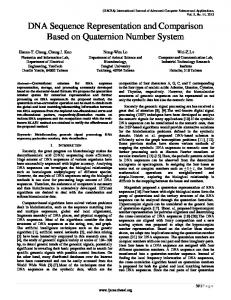
The internal force Fint dictates the regularity of the contour, whereas the external force Fext pulls it toward the desired image feature. We call Fext the potential force field, because it is the vector field that pulls the evolving contour toward the desired feature (edges) in the image. Figure 2.1(c) shows the potential force field, which is the negative gradient magnitude of the edge map in Figure 2.1(b). Figure 2.1(d) zooms in the area within the square box shown in Figure 2.1(c). The snake algorithm gains its popularity in the computer vision community because of the following characteristics: 1. It is deformable, which means it can be applied to segment objects with various shapes and sizes. 2. It guarantees a smooth and closed boundary of the object. 3. It has been proven very useful in motion tracking for video. The major drawbacks associated with the snake’s edge-based approach are: 1. It is very sensitive to noise because it requires the use of differential operators to calculate the edge map. 2. The potential forces in the potential force field are only present in the close vicinity of high values in the edge map. 3. It utilizes only the local information along the object boundaries, not the entire image. Hence, for the snake algorithm to converge to a desirable result, the initial contour must be placed close enough to the true boundary of the object. Otherwise, the evolving contour might stop at undesirable spurious edges or the contour might not move at all if the potential force on the contour front is not present. As a result, the initial contour is often obtained manually. This is a key pitfall of the snake method.

2.2.4.1 Variations of classical snakes Many efforts have been made to address the limitations of the original snakes method. For example, to help the snake move or avoid being trapped by spurious isolated edge points, Cohen’s balloon snake approach [36] added another artificial inflation force to the external force component of Equation (2.30). Thus, the balloon snake’s external force becomes


Chapter 2:


23

b.

a.

c.

b.

d.

Figure 2.1 (a) Original image; (b) edge map derived from the original image (a); (c) potential force field: the negative gradient of the edge map (b); (d) zoom in of area within the square box in (c).

Fext = -—P( x , y ) + Fconst nˆ ,

(2.33)

where Fconst is an arbitrary constant and nˆ is the unit normal vector on the contour front. However, the balloon snake has limitations. Although the balloon snake aims to pass through edges that are too weak with respect to the inflation force Fconst nˆ , adjusting the strength of the balloon force is difficult because it must be large enough to overcome the weak edges and noises but small enough not to overwhelm a legitimate boundary. Besides, the balloon force is image independent; i.e., it is not derived from the image. Therefore, the contour will continue to inflate at the points where the true boundary is missing or weaker than the inflation force. Xu and Prince [50, 39] introduced a new external force for edge-based snakes called the gradient vector flow (GVF) snake. In their method, instead


24


of directly using the gradient of the edge map as the potential force field, they diffuse it first to obtain a new force field that has a larger capture range than the gradient of the edge map. Figures 2.2(a) and (b) depict the gradient of an edge map and the Xu and Prince’s new force field, respectively. Comparing the two figures, we observe that the Xu and Prince’s vector forces gradually decrease as they are away from the edge pixels, whereas the vector forces in the gradient of the edge map exist only in the neighboring pixels of the edge pixels. As a result, there are no forces to pull a contour that is located at the pixels far away from the edge pixels in the gradient of the edge map field, but the contour may experience some forces at the same location in the Xu and Prince’s force field. Two other limitations associated with the parametric representation of the classical snake algorithm are the need to perform reparameterization and topological adaptation. It is often necessary to dynamically reparameterize the snake in order to maintain a faithful delineation of the object boundary. This adds computational overhead to the algorithm. In addition, when the contour fragments need to be merged or split, it may require a new topology and, thus, the reconstruction of the new parameterization. McInerney and Terzopoulos [51] have proposed an algorithm to address this problem.

2.2.5

Curve evolution theory

In this subsection, we explain how to control the motion of a propagating contour using the theory of curve evolution. In particular, we present two examples of the motion for a propagating curve that are commonly used in active contour schemes for image segmentation. Denote a family of smooth contours as È x( p , t) ˘ C( p , t) = Í ˙, Î y( p , t ) ˚

(2.34)

where p Œ[0,1] parameterizes the set of points on each curve, and t Œ[0, •) parameterizes the family of curves at different time evolutions. With this parameterization scheme, a closed contour has the property that C(0, t) = C(1, t) " t.

(2.35)

We are interested in finding an equation for the propagating motion of a curve that eventually segments the image. Assume a variational approach for image segmentation formulated as finding the curve C* such that C* = argmin J(C), C

(2.36)


Chapter 2:


25

a.

b. Figure 2.2 Two examples of the potential force fields of an edge map: (a) gradient of the edge map; (b) Xu and Prince’s GVF field.

where J is an energy functional constructed to capture all the criteria that lead to the desired segmentation. The solution to this variational problem often involves a partial differential Equation (PDE). Let F(C) denote an Euler-Lagrange equation such that the first variation of J(C) with respect to the contour C is zero. Under general assumptions, the necessary condition for C to be the minimizer of J(C) is that F(C) = 0. The solution to this necessary condition can be computed as the steady state solution of the following PDE [52] ∂C = F(C). ∂t

(2.37)

This equation is the curve evolution equation or the flow for the curve C . The form of this equation indicates that F(C) represents the “force” acting upon the contour front. It can also be viewed as the velocity at which the


26


contour evolves. Generally, the force F has two components. As depicted in Figure 2.3, Fnˆ is the component of F that points in the normal direction with respect to the contour front, and Ftˆ is the (other) component of F that is tangent to C. In curve evolution theory, we are only interested in Fnˆ because it is the force that moves the contour front forward (or inward), hence changing the geometry of the contour. The flow along Ftˆ , on the other hand, only re-parameterizes the curve and does not play any role in the evolution of the curve. Therefore, the curve evolution equation is often reduced to just the normal component as ∂C = F nˆ , ∂t

(2.38)

where F is called the speed function. In principle, the speed function depends on the local and global properties of the contour. Local properties of the contour include local geometric information such as the contour’s principal curvature k or the unit normal vector nˆ of the contour. Global properties of the curve depend on its shape and position. Coming up with an appropriate speed function, or equivalently the curve evolution equation, for the image segmentation underlies much of the research in this field. As an example, consider the Euclidean curve shortening flow given by ∂C = k nˆ . ∂t

(2.39)

This flow corresponds to the gradient descent along the direction in which the Euclidean arc length of the curve

Fn

Ft

Figure 2.3 The normal and tangential components of a force on the contour front.


Chapter 2:


L=

Ú ds

27

(2.40)

C

decreases most rapidly. As shown in Figure 2.4, a jagged closed contour evolving under this flow becomes smoother. Flow (2.39) has a number of attractive properties, which make it very useful in a range of image-processing applications. However, it is never used alone because if we continue the evolution with this flow, the curve will shrink to a circle, then to a point, and then finally vanishes. Another example illustrates some of the problems associated with a propagating curve. Consider the curve-evolution equation ∂C = Vonˆ , ∂t

(2.41)

where Vo is a constant. If Vo is positive, the contour inflates. If Vo is negative, the contour evolves in a deflationary fashion. This is because it corresponds to the minimization of the area within the closed contour. As seen in Figure 2.5, most curves evolving under the constant flow (2.41) often develop sharp points or corners that are nondifferentiable (along the contour). These singularities pose a problem of how to continue implementing the next evolution of the curve because the normal to the curve at a singular point is ambiguous. However, an elegant numerical implementation through the level set method provides an “entropy solution” that solves this curve evolution problem [53, 54, 46, 47]. Malladi et al. [38] and Caselles et al. [55] utilized both the curvature flow (2.39) and the constant flow (2.41) in their active contour schemes for image segmentation because they are complementary to each other. Whereas the constant flow can create singularities from an initial smooth contour, the curvature flow removes them by smoothing the contour in the process.

Figure 2.4 Flow under curvature: a jagged contour becomes smoother.


28


Figure 2.5 Flow with negative constant speed deflates the contour.

2.2.6

Level set method

Given a current position for the contour C and the equation for its motion such as the one in (2.37), we need a method to track this curve as it evolves. In general, there are two approaches to track the contour, the Lagrangian and the Eulerian approaches. The Lagrangian approach is a straightforward difference approximation scheme. It parameterizes the contour discretely into a set of control points lying along the moving front. The motion vectors, derived from the curve-evolution equation through a difference approximation scheme, are then applied to these control points to move the contour front. The control points then advance to their new locations to represent the updated curve front. Though this is a natural approach to track the evolving contour, the approach suffers from several problems [56]: 1. This approach requires an impractically small time step to achieve a stable evolution. 2. As the curve evolves, the control points tend to “clump” together near high curvature regions, causing numerical instability. Methods for control points reparameterization are then needed, but they are often less than perfect and hence can give rise to errors. 3. Besides numerical instability, there are also problems associated with the way the Lagrangian approach handles topological changes. As the curve splits or merges, topological problems occur, requiring ad hoc techniques [51, 57] to continue to make this approach work. Osher and Sethian [53, 54, 46, 47] developed the level set technique for tracking curves in the Eulerian framework, written in terms of a fixed coordinate system. There are four main advantages to this level set technique: 1. Since the underlying coordinate system is fixed, discrete mesh points do not move; the instability problems of the Lagrangian approximations can be avoided. 2. Topological changes are handled naturally and automatically. 3. The moving front is accurately captured regardless of whether it contains cusps or sharp corners.


Chapter 2:


29

4. The technique can be extended to work on any number of spatial dimensions. The level set method [46] implicitly represents the evolving contour C(t) by embedding it as the zero level of a level set function f : R 2 ¥ [0, •) Æ R , i.e.,

{

}

C(t) = ( x , y ) Œ W : f ( x , y , t) > 0 .

(2.42)

Starting with an initial level set function f (t = 0), we then evolve f (t) so that its zero level set moves according to the desired flow of the contour. Based on the convention that this level set graph has negative values inside C and positive values outside C, i.e.,

{

}

{

}

inside(C) = W1 = ( x , y ) Œ W : f ( x , y , t) > 0 , outside(C) = W 2 = ( x , y ) Œ W : f ( x , y , t) < 0 ,

(2.43) (2.44)

the level set function f can be implemented as the signed Euclidean distance to the contour C. For details about how to implement the Euclidean distance to a contour, see {58, 47]. Using the standard function 1, if f ≥ 0 H (f ) = ÏÌ0, if f < 0 , Ó

(2.45)

we can conveniently mask out the image pixels that are inside, outside, or on the contour C. For instance, the function H (f ) represents the binary template of the image pixels that are inside or on the contour. The function 1 - H (f ) represents the binary template of the image pixels that are strictly outside the contour. To select only the pixels that are on the contour C, we can use H (f ) - [1 - H ( -f )] . To facilitate numerical implementation, however, the regularized Heaviside function and its derivative, the regularized delta function, are often used instead. Define the regularized Heaviside function by H Œ(f ) =

1È 2 Êfˆ˘ 1 + arctan Í Ë Œ¯ ˙˚ 2Î p

(2.46)

then the regularized delta function is d Œ(f ) =

d H (f ), df Œ

(2.47)


30


=

1È Œ ˘ . p ÍÎ Œ2 +f 2 ˙˚

(2.48)

The functions H Œ(f ) , 1 - H Œ(f ) , and d Œ(f ) are to represent the templates of the image pixels that are inside, outside, and on the contour C, respectively. By defining the sign of the level set function f to be positive inside and negative outside the contour, the unit normal vector n of the contour C, defined as

n=

—f , —f

(2.49)

will point inward as shown in Figure 2.6. Furthermore, the curvature k along the contour, defined as Ê —f ˆ fxxfy2 - 2fxfyfxy + fyyfx2 k = div (n) = div Á 3/2 ˜= Ë —f ¯ f2 + f2

(

x

y

)

(2.50)

is positive where the unit normal vectors diverge. On the other hand, the curvature of the contour is negative if the unit normal vectors converge (see Figure 2.6).

2.2.7

Geometric active contours

Based on the theory of curve evolution [59], geometric active contours [38, 48] evolve the curves using only geometric measures, such as the curvature and the normal vectors, resulting in a contour evolution that is independent of the curve’s parameterization. Therefore, there is no need for reparameterization. In addition, the geometric active contour method can be implicitly C :φ = 0

n φ>0 κ>0

κ

Content-based image sequence representation - omni.isr.tecnico

Content-based image sequence representation - omni.isr.tecnico

Suggest Documents

CONTENT-BASED VIDEO SEQUENCE REPRESENTATION - Image

CONTENT-BASED VIDEO SEQUENCE REPRESENTATION - Image ...

ContentBased Access to Medical Image Collections - Google Sites

Hypergraph-based Image Representation

DNA Sequence Representation and Comparison

Structural Image Representation for Image ... - Semantic Scholar

Adaptive image sequence resolution

RESOLUTION-INVARIANT IMAGE REPRESENTATION ... - CiteSeerX

histopathology image representation for automatic

Stylized multiresolution image representation - CiteSeerX

Ontology-based Image Representation

Cognitive Image Representation Based on

JOY: protein sequence-structure representation and analysis

JOY: protein sequence-structure representation and analysis

Matrix Representation of Bi-Periodic Jacobsthal Sequence

Fractal Hash Sequence Representation and Traversal - CiteSeerX

DNA sequence representation without degeneracy - BioMedSearch

A Deep Conventional Image Representation for Image ... - Lixin Duan

Learning High-level Image Representation for Image Retrieval via ...

Critiquing Knowledge Representation in Medical Image ...

Learning Hierarchical Image Representation with Sparsity, Saliency ...

Kernel Sparse Representation for Image Classification ... - CiteSeerX

An Image Multiresolution Representation for ... - Semantic Scholar

Knowledge Representation for Image Feature Extraction