Contests with a Non-Convex Strategy Space Doron Klunover Ariel University John Morgan University of California, Berkeley November 2018 Abstract We characterize the Nash equilibria of a class of two-player contests with "lumpy" effort. Our main result shows that under quite reasonable conditions, constraints on the players' choice sets heighten competition. This stands in sharp contrast to the conventional wisdom that regulation decreases competition, but appears to be consistent with anecdotal evidence. Examples of this phenomenon include arms control, rules and regulations in sports, and drug wars. We also show that a constraint on available strategies can benefit a player. Keywords: Contests; Non-convex strategy space JEL classification numbers: C72, F51.
Corresponding author:
[email protected]
1
1. Introduction The standard assumption in contest theory that players have a convex choice set may be a reasonable assumption when units of effort are sufficiently small, but there are many important contexts in which this assumption does not hold. For instance, it may be possible for a country to contain an overseas crisis using a small number of aircraft, but getting them there and maintaining them may require the use of an aircraft carrier. Thus, the actual choice is between a large operation and no operation at all. Likewise, there may be a large fixed cost in supplementing air power with "boots on the ground". More generally, the choice set may be further constrained by rules, laws and regulations, technological constraints, political constraints and the like. Our main result suggests that under reasonable conditions such strategic constraints heighten competition. We use a stylized model that may need significant modification to completely describe any given situation. Nevertheless, numerous real-world examples in various contexts can be explained by the model. Moreover, the model improves on those in the existent literature, which usually assume away problems of “granularity” of effort in contests. This is further discussed in the review of the literature. In particular, we consider two types of simultaneous two-player contests with non-increasing return on effort and a prize with a common value (or similar values). The first is a symmetric strategy contest in which both players have the same non-
2
convex choice set of efforts (as perhaps in the case of the Cold War). The structure of the choice set that we consider is quite general. For instance, it can contain two separate convex subsets or it may be entirely discrete. The second type is an asymmetric strategy contest in which one player has a convex choice set of efforts while the other player's is non-convex, such as the case of the Taliban forces that have more flexible options than the Western coalition it faces. We present a complete characterization of the Nash equilibria of these contests. Our main result shows that under quite reasonable conditions deleting strategies from the players' strategy space heightens competition. In general, this result offers insight into the effect of strategic constraints on various situations that can be viewed as contests. One example is the offside rule in soccer that limits the set of possible positions for scoring a goal, but is considered to improve the competitiveness of the game. There are similar rules in other (team and individual) sports such as swimming, basketball, etc. An additional example in a different context is the Strategic Arms Limitation Talks (SALT) between the Cold War superpowers that accelerated development of new nuclear delivery technologies. Other attempts at arms control apparently had a similar outcome.1 Furthermore, in the asymmetric strategy contest, the strategic constraints allow the constrained player to make some sort of commitment. However, given that commitment usually has no value in the symmetric convex contest, she does not
1
Such as the Washington Naval Treaty discussed in detail later in the text.
3
benefit from such constraints. Nevertheless, we show that under some circumstances it is preferable to be the constrained player. The rest of the paper is structured as follows: In the remainder of this section, we present a survey of the literature. In section 2, we describe the general model. Section 3 characterizes equilibria in the symmetric strategy contest and derives conditions under which constraints on available strategies heighten competition. Section 4 analyzes the asymmetric strategy contest and section 5 further generalizes our results. Section 6 concludes. Review of the literature Our model is related to the extensive and still growing literature on contests, which has been surveyed by Konrad (2009) and more recently by Corchón and Serena (2018). The assumptions commonly made in the literature are that players have a convex strategy space and that effort exhibits non-increasing returns to scale. These assumptions are usually made for the sake of tractability and analytic convenience. In settings where effort exhibits increasing returns, standard solution methods fail. In this case, researchers approximate the strategy space by considering the limit of a sequence of discretized versions of the game.2 Baye et al. (1994) were the first to apply this method to characterizing the mixed strategy equilibria in the Tullock
2
Technically, the equilibrium characterization offered in these works represents the limit of a discrete strategy space rather than a convex one. It is an open question as to whether the limit equilibrium coincides with a real equilibrium. See Dasgupta and Maskin (1986) for a careful analysis of the issue.
4
contest (Tullock, 1980), in which return on effort is greater than two.3 Later studies that applied the same method include Amaldoss and Jain (2002) and Dechenaux et al. (2006). In their models, the non-convexity of strategies is merely a tool used to examine the equilibrium rather than a feature of interest on its own. In contrast, nonconvex strategy spaces are the present model’s main focus, rather than a convenience. To be precise, we focus on contests with non-increasing return on effort and a linear cost function for effort, which implies that the effective cost of effort is increasing and convex,4 as in the canonical models presented by Dixit (1987), Tullock (1980) and Skaperdas (1996). To the best of our knowledge, the convexity assumption regarding the strategy space has not been relaxed previously. A closely related model is Dubey (2013). He analyzed an all-pay auction with asymmetric players and incomplete information, in which players have a binary choice set. The restriction on the strategy space is intended mainly to permit equilibrium characterization with asymmetries and private information rather than being of interest in itself. We examine more general types of non-convexities and contest success functions. The tradeoff for adopting greater generality is that we must exclude private information as a possibility. Thus, one can view Dubey (2013) as the private information analog to our model. 2. The model 3
See Alcade and Dahm (2010) and Ewerhart (2015) for the complete characterization of these equilibria. 4 Without loss of generality, we also assume that marginal cost equals 1.
5
Two risk-neutral players compete for a prize (the objective of success) with a common value v. Each player 𝑖 ∈ {1,2} chooses an irreversible non-negative effort 𝑒𝑖 from the choice set 𝑆𝑖 . There are two types of choice sets: 1) a convex interval 𝑆𝑐 = [0,∞) and 2) a non-convex subset of Sc, 𝑆𝑛𝑐 (⊂ 𝑆𝑐 ). Other than non-convexity, 𝑆𝑛𝑐 is completely arbitrary with no additional restrictions. For example, it may contain two separate convex subsets or, alternatively, may be completely discrete. The usual form of analysis assumes that both players have the same convex choice set. We instead consider two alternatives: 1) Both players have the same non-convex choice set; and 2) one player’s choice set is convex while the other’s is non-convex. We shall refer to the first situation as a symmetric strategy contest and the second as an asymmetric strategy contest. Let 𝑝(𝑒𝑖 , 𝑒𝑗 ) be the probability that player 𝑖 ∈ {1,2} will win. We shall make use of the term contest success function (or CSF) to describe p. It is well known that some restrictions are needed to ensure that there is a unique equilibrium when identical competitors with convex strategy spaces compete.5 We retain these restrictions on the CSF throughout the analysis. This is done for both analytic tractability and, more importantly, to allow for a ready comparison of our results to those in the literature, thus ensuring that any difference depends purely on dropping the convexity assumption. To complete the model, we assume that 𝑝 is twice continuously differentiable when 𝑒𝑖 + 𝑒𝑗 > 0, and that it also satisfies the usual properties: 5
See Dixit (1987) and Baye and Shin (1999).
6
2
𝜕𝑝 𝑑 𝑝 (1) 𝑝(𝑒𝑗 , 𝑒𝑖 ) = 1 − 𝑝(𝑒𝑖 , 𝑒𝑗 ) and 𝑝𝑖 ≡ 𝜕𝑒 > 0 and 𝑝𝑖𝑖 ≡ 𝜕𝑒2 < 0 in the interior of 𝑖
𝑖
its domain. To summarize, player i's problem is: (2) max 𝐸𝜋(𝑒𝑖 ; 𝑒𝑗 ) such that 𝑒𝑖 ∈ 𝑆𝑖 , where 𝐸𝜋(𝑒𝑖 , 𝑒𝑗 ) = 𝑝(𝑒𝑖 , 𝑒𝑗 )𝑣 − 𝑒𝑖 ∀𝑖 ∈ {1,2}. 𝑒𝑖
The remainder of the paper characterizes the equilibria when we relax the assumption of continuous available strategies. In the next section, we compute the analog of the main results in contest theory, in a setting where the two competitors are identical. 3. Symmetric strategy contests As a benchmark, Figure 1 illustrates the case in which strategy spaces are convex. It is well known that in this case there is a unique symmetric interior solution which we denote by 𝑒∗𝑐 .
7
e2
450 BR1
𝑒∗𝑐
BR2 e1
𝑒𝑐∗
Figure 1: Best response curves in the symmetric convex contest We now compare this to a situation in which the set of available strategies is identical, but non-convex. We reproduce the standard equilibrium analysis with only this modification as follows: First, we present Lemmas 0-2 which present important equilibria features and some additional technical results needed for the rest of the analysis. We then present Proposition 1 which shows that under quite reasonable conditions a constraint on the player strategy space increases competition. Finally, at the end of this section, Proposition 2 characterizes the complete equilibria structure more generally (without requiring the conditions in Proposition 1) and is followed by Corollary 1 which derives sufficient conditions to reproduce the result shown in Proposition 1. Our analysis therefore begins with Lemma 0. Suppose that the players' strategy spaces are S1=S2=Snc. When ec* is contained in Snc, it is trivial to show that the
8
choice of ec* by both players remains an equilibrium. However, it is unclear whether the deletion of strategies might also produce new equilibria. In Lemma 0, we claim that, regardless of the structure of Snc, no new equilibria appear, but to formally demonstrate this will require Lemma 1, which applies regardless of whether or not ec* is in Snc. For now, we postpone the discussion and merely note the following: Lemma 0 In the symmetric strategy contest, if ec* is contained in Snc, then it is the unique equilibrium. Herein we assume that ec* is not contained in Snc and do not impose any other restrictions on the structure of Snc. To this end, define 𝑒 and 𝑒̅ to be the efforts that bracket the equilibrium point under convex effort. That is, ∄𝑒 ∈ 𝑆𝑛𝑐 |𝑒 ∈ (𝑒, 𝑒̅ ), where 0 ≤ 𝑒 ≤ 𝑒𝑐∗ ≤ 𝑒̅ . We restrict what follows to the non-trivial case, in which 𝑒 and 𝑒̅ exist. We are now in a position to present Lemma 1: Lemma 1 In a symmetric strategy contest with non-convex effort, each player‘s equilibrium effort is an element from the set {𝑒, 𝑒̅ }. Lemma 1 implies that, regardless of the full set of elements of Snc, it suffices to consider only the symmetric 2x2 contest where choice is limited to {𝑒, 𝑒̅ }.6 This
6
More precisely, Lemma 1 implies that the set of equilibria in the original game is a subset of the set of equilibria in the 2x2 game. However, it can be readily shown that these two sets coincide. Formally, this is demonstrated in the proof of Proposition 2.
9
greatly simplifies the analysis. Finally, notice that Lemma 0 follows immediately since, when ec* is contained in Snc, the set {𝑒, 𝑒̅ } becomes a singleton.7 While Lemma 1 significantly reduces the candidates for equilibrium strategies, it remains to characterize the resulting set of equilibria. It proves useful to define a threshold effort level 𝑒̂ with the following properties: (1) When her rival chooses 𝑒, a player is indifferent between choosing the threshold and 𝑒. (2) Likewise, when her rival chooses 𝑒̂ , the player is again indifferent between choosing 𝑒̂ and 𝑒. Formally, 𝑒̂ solves 𝐸𝜋(𝑒̂ , 𝑒′) = 𝐸𝜋(𝑒, 𝑒′) for 𝑒′ ∈ {𝑒̂ , 𝑒}. The expression 𝑒̂ is well-defined so long as 𝑒 is not too large. Otherwise, no interior solution exists for solving the indifference condition. Define 𝛿 to be the maximal value of 𝑒 such that there exists a (weak) interior threshold, i.e. δ solves 𝐸𝜋(0, 𝑒′) = 𝐸𝜋(𝛿, 𝑒′) for 𝑒 ′ ∈ {0, 𝛿}. Notice that the left-hand side of the indifference condition takes account of the fact that the lowest possible threshold occurs when 𝑒̂ = 0. Moreover, it can readily be seen that 𝑒̂ is decreasing with respect to 𝑒. Lemma 2 formally establishes the properties of the threshold. Lemma 2 There exists a unique 𝛿 which is not greater than v/2. If 𝑒 ≤ 𝛿, then there exists a unique 𝑒̂ ∈ [0,𝑒∗𝑐 ) which is monotonically decreasing in 𝑒; otherwise ∄𝑒̂ . To obtain the next result in Proposition 1, we need additional assumptions that impose technical restrictions on the CSF. These assumptions must hold for a CSF defined for any given number of players while the CSF in (1) is defined only for 7
Note that when ec* is contained in Snc, by the definition of e and 𝑒, the set {𝑒, 𝑒̅} is not uniquely defined; it can be either {𝑒𝑐∗ , 𝑒̅} when 𝑒𝑐∗ < 𝑒̅ or {𝑒, 𝑒𝑐∗ } when 𝑒 < 𝑒𝑐∗ or {𝑒𝑐∗ }. Lemma 1 holds in all of these cases.
10
two. Therefore, to ease the burden of notation, we note the assumptions but refer the reader to Skaperdas (1996) for the complete and formal definitions. Specifically: Assumption 1 Contests among a small numbers of players are qualitatively similar to those among a large number (see Skaperdas, 1996; A4). Assumption 2 The outcome in a contest among any subset of players should not depend on the efforts of the players not participating in the contest (see Skaperdas, 1996; A5). Assumption 3 The players' winning probabilities are homogenous of degree zero in effort (see Skaperdas, 1996; A6). We formally define "a symmetric bracketing of the strategy space" as 𝑒 − 𝑒𝑐∗ = 𝑒𝑐∗ − 𝑒 which allows to state the following proposition: Proposition 1 Under Assumptions 1-3, in any symmetric strategy contest with non-convex choices, a symmetric bracketing of the strategy space heightens competition. Specifically, the unique equilibrium effort in pure strategies is then 𝑒.8 Notice that Skaperdas (1996, Theorem 2) shows that Tullok’s CSF (Tullok, 1980) is the only one that satisfies both (1) and Assumptions 1-3.9 This class of CSF is perhaps the most commonly used CSF in the literature and is formally defined as:
8
Notice that pi=xi/(xi+ xj) is an exception, since in that special case a symmetric bracketing of the strategy space results in a continuum of equilibria consisting of arbitrary weights given to {𝑒, 𝑒̅}. 9 Notice that, in addition to Assumptions 1-3, Skaperdas (1996) needs three more assumptions to hold for a CSF defined for any given number of players in order to axiomatize the Tullock CSF. The CSF in (1) satisfies these assumptions for the case of two players.
11
𝑒𝑖𝑟 𝑖𝑓 𝑒𝑖 + 𝑒𝑗 > 0, 𝑒𝑖𝑟 + 𝑒𝑗𝑟 (3) 𝑝(𝑒𝑖 , 𝑒𝑗 ) = , 1 𝑜𝑡ℎ𝑒𝑟𝑤𝑖𝑠𝑒 { 2 } where 𝑟 ≤ 1.10 Note that it is well known that 𝑒∗𝑐 =
𝑟𝑣 4
in this case.
Proposition 1 can perhaps explain the outcome of the Washington Naval Treaty, in which the victors in WWI agreed to limit the arms race by imposing specific constraints on naval construction. However, in many ways, the development of aircraft carriers by the US and Japan was accelerated by these constraints, since budgets and hulls were now diverted from banned capital ship development to aircraft carriers and submarines. In particular, several American and Japanese carriers were constructed from battlecruiser and battleship hulls. As is well known, aircraft carriers turned out to be one of the deadliest weapons of the 20th century. A further example is perhaps the Anabolic Steroid Control Act (ASCA) passed in 1990 which was intended to end “cheating” in sports. However, far from eliminating the “cheating”, it is commonly argued that the use of stronger and riskier anabolic steroids and performance-enhancing drugs (PEDs) that clearly (and unethically) heighten competitive ability has proliferated since the ASCA became law.11 More generally, in Proposition 2 we characterize the equilibrium structure for any symmetric strategy contest and in Corollary 1 we note the sufficient and necessary 10 11
Note that the concavity of p, as stated in (1) (i.e., 𝑝𝑖𝑖 < 0) , may be violated when r>1. See Ryvkin (2013) for a model of contests with doping.
12
condition under which constraints on the players' strategy space heighten competition. Proposition 2 A symmetric strategy contest with non-convex choices has a unique equilibrium in pure strategies: a. Effort is e when 𝑒>δ or 𝑒̂ e. 12 It therefore follows that: Corollary 1 In any symmetric strategy contest with non-convex choices, constraints on the players' strategy space heighten competition when e 𝐸𝜋(𝑒̅, 𝐵𝑅1 (𝑒̅ ) ) and 𝐸𝜋 (𝑒, 𝐵𝑅1 (𝑒)) ≥ 𝐸𝜋(𝑒̅, 𝐵𝑅1 (𝑒)), then effort is (𝐵𝑅1 (𝑒), 𝑒); if 𝐸𝜋 (𝑒, 𝐵𝑅1 (𝑒̅)) ≤ 𝐸𝜋(𝑒̅ , 𝐵𝑅1 (𝑒̅ )) and 𝐸𝜋 (𝑒, 𝐵𝑅1 (𝑒)) < 𝐸𝜋(𝑒̅, 𝐵𝑅1 (𝑒)), then effort is (𝐵𝑅1 (𝑒̅ ), 𝑒̅ ); if 𝐸𝜋 (𝑒, 𝐵𝑅1 (𝑒̅)) ≤ 𝐸𝜋(𝑒̅ , 𝐵𝑅1 (𝑒̅ )) and 𝐸𝜋 (𝑒, 𝐵𝑅1 (𝑒)) ≥ 𝐸𝜋( 𝑒̅, 𝐵𝑅1 (𝑒)), then the possible efforts are (𝐵𝑅1 (𝑒), 𝑒) and (𝐵𝑅1 (𝑒̅ ), 𝑒̅ ); otherwise there does not exist a Nash equilibrium in the case of pure strategies. Corollary 2 implies that in an asymmetric strategy contest, and regardless of player 2's full set of elements, it is sufficient to identify the signs of 𝐸𝜋 (𝑒, 𝐵𝑅1 (𝑒̅ )) − 𝐸𝜋(𝑒̅, 𝐵𝑅1 (𝑒̅)) and 𝐸𝜋 (𝑒, 𝐵𝑅1 (𝑒)) − 𝐸𝜋(𝑒̅ , 𝐵𝑅1 (𝑒)). We restrict what follows to the non-trivial case, in which 𝑒̅ < 𝑣.13 In order to analyze the asymmetric strategy contest, we impose Assumptions 1-3 on the CSF in the rest of this section.
13
Notice that 𝐸𝜋 (𝑒, 𝐵𝑅1 (𝑒̅)) > 𝐸𝜋(𝑒̅, 𝐵𝑅1 (𝑒̅ )) and 𝐸𝜋 (𝑒, 𝐵𝑅1 (𝑒)) > 𝐸𝜋 (𝑒̅, 𝐵𝑅1 (𝑒)) for all 𝑒̅ ≥ 𝑣.
Therefore, the equilibrium is (𝐵𝑅1 (𝑒), 𝑒) when 𝑒̅ ≥ 𝑣.
15
In order to characterize the equilibria in the asymmetric strategy contest, we need to define three threshold effort levels: (1) 𝑒𝑅 which solves 𝐸𝜋(𝑒𝑅 , 𝐵𝑅1 (𝑒̅ )) − 𝐸𝜋(𝑒̅ , 𝐵𝑅1 (𝑒̅ )) = 𝐸𝜋(𝑒𝑅 , 𝐵𝑅1 (𝑒𝑅 )) − 𝐸𝜋(𝑒̅, 𝐵𝑅1 (𝑒𝑅 ));
(2)
𝑒0 which
solves
𝐸𝜋(𝑒0 , 𝐵𝑅1 (𝑒0 )) = 𝐸𝜋(𝑒̅, 𝐵𝑅1 (𝑒0 )); and (3) 𝑒00 which solves 𝐸𝜋(𝑒00 , 𝐵𝑅1 (𝑒̅) ) = 𝐸𝜋( 𝑒̅, 𝐵𝑅1 (𝑒̅)). For a given 𝑒̅ , the terms: 𝐸𝜋 (𝑒, 𝐵𝑅1 (𝑒̅ )) − 𝐸𝜋(𝑒̅ , 𝐵𝑅1 (𝑒̅ )) and 𝐸𝜋 (𝑒, 𝐵𝑅1 (𝑒)) − 𝐸𝜋 (𝑒̅, 𝐵𝑅1 (𝑒)) and the resulting thresholds defined above are pictured in Figure 2 (and formally described by Lemma 3 and Corollary 3 in the appendix) .
𝐸𝜋 (𝑒, 𝐵𝑅1 (𝑒̅)) − 𝐸𝜋(𝑒̅, 𝐵𝑅1 (𝑒̅)), 𝐸𝜋 (𝑒, 𝐵𝑅1 (𝑒)) − 𝐸𝜋 (𝑒̅, 𝐵𝑅1 (𝑒))
W 0
𝒆𝟎 𝒆𝟎𝟎 𝒓𝒗 𝟒
𝒆𝑹
𝑒
Figure 2: The shape of 𝐸𝜋 (𝑒, 𝐵𝑅1 (𝑒̅ )) − 𝐸𝜋(𝑒̅ , 𝐵𝑅1 (𝑒̅ )) and 𝐸𝜋 (𝑒, 𝐵𝑅1 (𝑒)) − 𝐸𝜋 (𝑒̅, 𝐵𝑅1 (𝑒)) when 𝑟 < 1.14 We are now in a position to characterize the set of equilibria in an asymmetric strategy contest with a non-convex choice space: 14
Notice that 𝑒𝑅 = 𝑒0 = 𝑒00 when 𝑟 = 1.
16
Proposition 3 Given that 𝑒̅ < 𝑣, under Assumptions 1-3, in any asymmetric strategy contest with non-convex choices, the Nash equilibria in pure strategies are as follows: a. Effort is (𝐵𝑅1 (𝑒̅ ), 𝑒̅ ) when 𝑒 < 𝑒0 b. Effort is (𝐵𝑅1 (𝑒), 𝑒) when 𝑒 > 𝑒00 c. Otherwise, both (𝐵𝑅1 (𝑒̅ ), 𝑒̅ ) and (𝐵𝑅1 (𝑒), 𝑒) are equilibrium efforts.15 Proposition 3 implies that, a gradual deletion of effort from the choice set can boost effort, as in the case of the symmetric strategy contest. However, unlike the case of the symmetric strategy contest, in which equilibrium in pure strategies is usually unique, there are two different Nash equilibria in pure strategies when 𝑒 is contained in the interval [𝑒0 , 𝑒00 ], where this interval is a singleton only when the exponent r in (3) is equal to 1. Notice that player 2 will always prefer to have a convex choice set of efforts, or more precisely, to be able to choose ec*. This is because in the symmetric convex contest, commitment has no value, and therefore a player does not benefit from any type of bracketing in the strategy space (Dixit, 1987; Baik and Shogren, 1992; Possajennikov, 2009). Nevertheless, in an asymmetric strategy contest, a player will prefer to be constrained in some circumstances. To see this, consider the following: When the equilibrium effort is (𝐵𝑅1(𝑒), 𝑒), player 1’s expected net payoff is larger than her rival’s (and even larger than the payoff in the standard symmetric convex 15
The structure of the equilibria in which player 2 mixes pure strategies is as follows: Given that r 𝐸π (𝑒, 𝐵𝑅1 (𝑒)) and 𝐸π(𝐵𝑅1 (𝑒), 𝑒) > 𝐸π(𝑒, 𝑒) > 𝐸π(𝑒𝑐∗ , 𝑒𝑐∗ ). 17
9
9
16
16
Notice that 𝐵𝑅1 ( ) = √
−
9 16
=
3 16
. Furthermore, it is also possible that (𝑒1∗ , 𝑒2∗ ) = (𝐵𝑅1 (𝑒̅), 𝑒̅ ) and
player 1’s expected net payoff will be larger than player 2’s. In particular, this can happen when r, the exponent in the CSF in (3), is sufficiently small (such that p1≈p2 and e1 0, BR1(e) satisfies player 1’s FOC for an interior maximum and therefore: 𝜕𝐸𝜋1 (𝐵𝑅1 (𝑒),𝑒) 𝜕𝑒1
(A.16)
=
𝑟−1 𝑟 𝑒
𝑟(𝐵𝑅1 (𝑒))
𝑟 2
(𝑒𝑟 +(𝐵𝑅1 (𝑒)) )
𝑣−1=0
↔ 𝑟 2
𝑣 𝑒𝑟 =
(𝑒𝑟 + (𝐵𝑅1 (𝑒)) ) 𝑟(𝐵𝑅1 (𝑒))
∀𝑒 > 0.
𝑟−1
Substituting the RHS of (A.16) into the nominator of the first term in the RHS of (A.15) results in: 𝑟
1
(A.17) 𝐸𝜋 (𝑒, 𝐵𝑅1 (𝑒)) = 𝑟 (𝑒𝑟 + (𝐵𝑅1 (𝑒)) )(𝐵𝑅1 (𝑒)) 1−𝑟
1
= 𝑟 (𝐵𝑅1 (𝑒) + 𝑒 𝑟 (𝐵𝑅1 (𝑒))
1−𝑟
−𝑒
) − 𝑒 ∀𝑒 > 0.
Taking the derivative of (A.17) with respect to e yields:
(A.18)
𝑑𝐸𝜋(𝑒,𝐵𝑅1 (𝑒)) 𝑑𝑒
1−𝑟 𝐵𝑅1 (𝑒) 1 𝑑𝐵𝑅1 (𝑒) + 𝑟 ( ) 𝑑𝑒 𝑒
= 𝑟(
=(
𝐵𝑅1 (𝑒) 𝑒
By (A.1), 𝐵𝑅1 (𝑒) > 𝑒 and
1−𝑟
)
𝑑𝐵𝑅1 (𝑒) 𝑑𝑒
+ (1 − 𝑟) (𝐵𝑅
𝑑𝑒
𝑟
)
1 (𝑒)
1 𝑑𝐵𝑅1 (𝑒)
−1+𝑟
𝑒
𝑑𝐵𝑅1 (𝑒) )−1 𝑑𝑒
(1 + (1 − 𝑟) (𝐵𝑅
> 0, and thus, by (A.18),
𝑒
1
𝑟
) ) ∀𝑒 > 0. (𝑒)
𝑑𝐸𝜋(𝑒,𝐵𝑅1 (𝑒)) 𝑑𝑒
≥ 0 ∀𝑒 > 0.
Given that 𝐵𝑅1 (𝑒) is increasing in 𝑒, 𝐸𝜋 (𝑒̅ , 𝐵𝑅1 (𝑒)) is decreasing in 𝑒. Therefore,
30
𝐸𝜋 (𝑒, 𝐵𝑅1 (𝑒)) − 𝐸𝜋 (𝑒̅ , 𝐵𝑅1 (𝑒)) is increasing in 𝑒 for all 𝑒 ≥ 0.28 Notice also that 𝑒̅
𝐸𝜋(0, 𝐵𝑅1 (0)) − 𝐸𝜋 (𝑒̅ , 𝐵𝑅1 (𝑒)) = 𝑒̅ − 𝑒̅+𝜀 𝑣 ≈ 𝑒̅ − 𝑣.
Proof of Lemma 3iii: We prove Lemma 3iii in two steps: First, we show that there 𝑟𝑣
exists a unique 𝑒𝑅 ∈ [0, 4 ) and then we find the sign of 𝐸𝜋(𝑒̅ , 𝐵𝑅1 (𝑒𝑅 )) − 𝐸𝜋(𝑒𝑅 , 𝐵𝑅1 (𝑒𝑅 )).
We thus begin by proving that there exists a unique 𝑒𝑅 : (A.19)
𝐸𝜋(𝑒𝑅 , 𝐵𝑅1 (𝑒̅ )) − 𝐸𝜋(𝑒̅ , 𝐵𝑅1 (𝑒̅ ))
= 𝐸𝜋(𝑒𝑅 , 𝐵𝑅1 (𝑒𝑅 )) − 𝐸𝜋(𝑒̅ , 𝐵𝑅1 (𝑒𝑅 )) ↔ 𝑝(𝑒𝑅 , 𝐵𝑅1 (𝑒̅ )) − 𝑝(𝑒̅ , 𝐵𝑅1 (𝑒̅ )) = 𝑝(𝑒𝑅 , 𝐵𝑅1 (𝑒𝑅 )) − 𝑝(𝑒̅ , 𝐵𝑅1 (𝑒𝑅 )
↔ 1 − 𝑝(𝑒̅ , 𝐵𝑅1 (𝑒̅ )) − (1 − 𝑝(𝑒𝑅 , 𝐵𝑅1 (𝑒̅ ))) = 1 − 𝑝(𝑒̅ , 𝐵𝑅1 (𝑒𝑅 ) − (1 − 𝑝(𝑒𝑅 , 𝐵𝑅1 (𝑒𝑅 )))
↔ 𝑝(𝐵𝑅1 (𝑒̅ ), 𝑒̅ ) − 𝑝(𝐵𝑅1 (𝑒̅ ), 𝑒𝑅 ) = 𝑝(𝐵𝑅1 (𝑒𝑅 ), 𝑒̅ ) − 𝑝(𝐵𝑅1 (𝑒𝑅 ), 𝑒𝑅 )
↔ 𝐸𝜋(𝐵𝑅1 (𝑒̅ ), 𝑒̅ ) − 𝐸𝜋(𝐵𝑅1 (𝑒𝑅 ), 𝑒̅ ) = 𝐸𝜋(𝐵𝑅1 (𝑒̅ ), 𝑒𝑅 ) − 𝐸𝜋(𝐵𝑅1 (𝑒𝑅 ), 𝑒𝑅 )
↔ 𝐵𝑅1 (𝑒̅ ) = 𝐵𝑅1 (𝑒𝑅 ). 29 𝑟𝑣 By the structure of 𝐵𝑅𝑖 described in (A.1)30, for any given 𝑒̅ ∈ ( 4 , 𝑣], there exists a 𝑟𝑣
unique 𝑒𝑅 ∈ [0, 4 ) that solves 𝐵𝑅1 (𝑒̅) = 𝐵𝑅1 (𝑒𝑅 ). 28
Notice that, 𝐵𝑅1 (0) = 𝜀 and thus 𝐸𝜋(0, 𝐵𝑅1 (0)) = 0 while 𝐸𝜋(𝜀, 𝐵𝑅1 (𝜀)) > 0 for 𝜀 > 0. This implies
that, 𝐸𝜋 (𝑒, 𝐵𝑅1 (𝑒)) − 𝐸𝜋 (𝑒̅, 𝐵𝑅1 (𝑒)) is increasing in e at e=0 despite the discontinuity of 𝐵𝑅1 (𝑒) at e=0. 29 Notice that 𝐸𝜋(𝐵𝑅1 (𝑒̅ ), 𝑒̅) > 𝐸𝜋(𝐵𝑅1 (𝑒𝑅 ), 𝑒̅) and 𝐸𝜋(𝐵𝑅1 (𝑒̅), 𝑒𝑅 ) < 𝐸𝜋(𝐵𝑅1 (𝑒𝑅 ), 𝑒𝑅 ) when 𝐵𝑅1 (𝑒̅ ) ≠ 𝐵𝑅1 (𝑒𝑅 ).
31
We now proceed to find the sign of 𝐸𝜋(𝑒̅ , 𝐵𝑅1 (𝑒𝑅 )) − 𝐸𝜋(𝑒𝑅 , 𝐵𝑅1 (𝑒𝑅 )). By the FOC for maximization of player 1: (A.20)
𝜕𝑝(𝐵𝑅1 (𝑒̅ ),𝑒̅ ) 𝜕𝑒1
=
𝜕𝑝(𝐵𝑅1 (𝑒𝑅 ),𝑒𝑅 ) 𝜕𝑒1
↔ 𝑒̅ 𝑟
𝑒𝑅 𝑟 = 2 2 (𝑒̅ 𝑟 + (𝐵𝑅1 (𝑒𝑅 ))𝑟 ) (𝑒𝑅 𝑟 + (𝐵𝑅1 (𝑒𝑅 ))𝑟 ) ↔ (𝑒𝑅 𝑟 + (𝐵𝑅1 (𝑒𝑅 ))𝑟 )√𝑒̅ 𝑟 = (𝑒̅ 𝑟 + (𝐵𝑅1 (𝑒𝑅 ))𝑟 )√𝑒𝑅 𝑟 ↔ ((𝐵𝑅1 (𝑒𝑅 ))𝑟 − √(𝑒̅ 𝑒𝑅 )𝑟 )(√𝑒̅ 𝑟 − √𝑒𝑅 𝑟 ) = 0 ↔ 𝐵𝑅1 (𝑒𝑅 ) = √𝑒̅ 𝑒𝑅 . Substituting 𝑒 = 𝑒𝑅 and (A.20) into (A.16) results in: 𝑟−1
(A.21)
𝑟(√𝑒̅ 𝑒𝑅 )
𝑒𝑅 𝑟
2 (𝑒𝑅 𝑟 +√(𝑒̅ 𝑒𝑅 )𝑟 )
𝑣=1
↔ 𝑟−1
𝑟(√𝑒̅ 𝑒𝑅 )
(√𝑒𝑟𝑅 + √𝑒̅ 𝑟 )
2
𝑣=1
↔ 𝑟(√𝑒̅𝑒𝑅 )𝑟−1 𝑣 = (√𝑒̅ 𝑟 + √𝑒𝑅𝑟 )2 . Also, substituting (A.20) into 𝐸𝜋(𝑒̅ , 𝐵𝑅1 (𝑒𝑅 )) − 𝐸𝜋(𝑒𝑅 , 𝐵𝑅1 (𝑒𝑅 )) results in: 30
Over the interval (0,v), 𝐵𝑅𝑖 is positive and has an approximate inverted U-shape with a unique maximum at 𝑟v/4. See Pérez-Castrillo and Verdier (1992) for a detailed analysis of the reaction functions in the Tullock contest.
32
𝐸𝜋(𝑒̅ , 𝐵𝑅1 (𝑒𝑅 )) − 𝐸𝜋(𝑒𝑅 , 𝐵𝑅1 (𝑒𝑅 ))
(A.22)
=(
𝑒̅ 𝑟 𝑒̅ 𝑟 + √(𝑒̅ 𝑒𝑅 )𝑟
=(
=
√𝑒̅ 𝑟 √𝑒̅ 𝑟 +√𝑒𝑅𝑟
−
−
𝑒𝑅 𝑟 𝑒𝑅 𝑟 + √(𝑒̅ 𝑒𝑅 )𝑟
√𝑒𝑅𝑟 √𝑒̅ 𝑟 +√𝑒𝑅𝑟
𝑒̅ 𝑟 − 𝑒𝑅 𝑟 (√𝑒̅ 𝑟 + √𝑒𝑅𝑟 )2
) 𝑣 − (𝑒̅ − 𝑒𝑅 )
) 𝑣 − (𝑒̅ − 𝑒𝑅 ) =
√𝑒̅ 𝑟 −√𝑒𝑅𝑟 √𝑒̅ 𝑟 +√𝑒𝑅𝑟
𝑣 − (𝑒̅ − 𝑒𝑅 )
𝑣 − (𝑒̅ − 𝑒𝑅 ).
Assuming that r≠0, substituting the LHS of (A.21) into the denominator of the first term of (A.22) results in: (A.23) 𝐸𝜋(𝑒̅ , 𝐵𝑅1 (𝑒𝑅 )) − 𝐸𝜋(𝑒𝑅 , 𝐵𝑅1 (𝑒𝑅 )) =
𝑒̅ 𝑟 −𝑒𝑅 𝑟 𝑟√(𝑒̅ 𝑒𝑅 )𝑟−1
− (𝑒̅ − 𝑒𝑅 ), where
𝑒̅ 𝑟 −𝑒𝑅 𝑟
− (𝑒̅ − 𝑒𝑅 )) = 𝑠𝑖𝑔𝑛 ( 𝑟−1
(A.24) 𝑠𝑖𝑔𝑛 (
𝑟√(𝑒̅ 𝑒𝑅 )
𝑒̅ 𝑟 −𝑒𝑅 𝑟 (𝑒̅ −𝑒𝑅 )√(𝑒̅ 𝑒𝑅 )𝑟−1
− 𝑟)
𝑒̅ 𝑟 − 𝑒𝑅 𝑟
= 𝑠𝑖𝑔𝑛 ( 1 𝑟 − 𝑟) = 𝑠𝑖𝑔𝑛 (𝑒̅ − 𝑒𝑅 )(𝑒̅ 𝑒𝑅 )−2 (𝑒̅𝑒𝑅 )2
= 𝑠𝑖𝑔𝑛
𝑟
𝑟
1 2
1 𝑒𝑅 2
𝑒̅ 2 𝑒 2 (𝑒 ) − ( 𝑒̅𝑅 ) 𝑅 𝑒̅ ) −( ) 𝑒 𝑒̅ ( 𝑅 (
−𝑟 . )
33
𝑒̅ 𝑟 − 𝑒𝑅 𝑟 1
1
𝑟 𝑒̅ 2 𝑒 2 ((𝑒 ) − ( 𝑒̅𝑅 ) )(𝑒̅ 𝑒𝑅 )2 ( 𝑅
−𝑟 )
Notice that
𝑟 𝑟 𝑒 𝑒̅ 2 ) −( ̅𝑅 )2 𝑒𝑅 𝑒 1 1 𝑒 𝑒̅ 2 ( ) −( ̅𝑅 )2 𝑒𝑅 𝑒
(
= 1 at r=1, and
𝑟 𝑟 𝑒 𝑒̅ 2 ) −( ̅𝑅 )2 𝑒𝑅 𝑒 1 1 𝑒 𝑒̅ 2 ( ) −( ̅𝑅 )2 𝑒𝑅 𝑒
(
→ 0 when r →0. Since
𝑟 𝑟 𝑒 𝑒̅ 2 ) −( ̅𝑅 )2 𝑒𝑅 𝑒 1 1 𝑒 𝑒̅ 2 ( ) −( ̅𝑅 )2 𝑒𝑅 𝑒
(
is
increasing and convex with respect to r over the interval 𝑟 ∈ (0,1]31, if 𝑟 ∈ (0,1) then 𝐸𝜋(𝑒̅ , 𝐵𝑅1 (𝑒𝑅 )) − 𝐸𝜋(𝑒𝑅 , 𝐵𝑅1 (𝑒𝑅 )) < 0. 32
QED
Lemma 3 implies the following corollary: Corollary 3 Given 𝑒̅ < 𝑣, there exists a unique tuple (𝑒0 ,𝑒00 ,eR). If r 𝑒0 > eR (𝑒00 = 𝑒0 = eR). By Corollary 2, Lemma 3 and Corollary 3, the Nash equilibria in the case of pure strategies shown in Proposition 3 is straightforward. Regarding equilibria in the case of mixed strategies: At 𝑞 = 1, 𝐸𝜋 (𝑒, 𝐵𝑅1 (𝑞𝑒 + (1 − 𝑞)𝑒)) − 𝐸𝜋 (𝑒, 𝐵𝑅1 (𝑞𝑒 + (1 − 𝑞)𝑒)) = 𝐸𝜋 (𝑒, 𝐵𝑅1 (𝑒)) − 𝐸𝜋 (𝑒̅ , 𝐵𝑅1 (𝑒)),
and
at
𝑞 = 0, 𝐸𝜋 (𝑒, 𝐵𝑅1 (𝑞𝑒 + (1 − 𝑞)𝑒)) − 𝐸𝜋 (𝑒, 𝐵𝑅1 (𝑞𝑒 + (1 − 𝑞)𝑒)) = 𝐸𝜋 (𝑒, 𝐵𝑅1 (𝑒̅ )) − 𝐸𝜋(𝑒̅ , 𝐵𝑅1 (𝑒̅ )). Since when 𝑟 < 1 and 𝑒 ∈ (𝑒0 , 𝑒00 ), by Lemma 3 and Corollary
2, 𝐸𝜋 (𝑒, 𝐵𝑅1 (𝑒̅)) < 𝐸𝜋(𝑒̅, 𝐵𝑅1 (𝑒̅))
and
𝐸𝜋 (𝑒, 𝐵𝑅1 (𝑒)) > 𝐸𝜋 (𝑒̅ , 𝐵𝑅1 (𝑒)),
by
the
Intermediate Value Theorem there exists 𝑞 ∈ (0,1) such that 𝐸𝜋 (𝑒, 𝐵𝑅1 (𝑞𝑒 + (1 − 𝑞)𝑒)) = 𝐸𝜋 (𝑒, 𝐵𝑅1 (𝑞𝑒 + (1 − 𝑞)𝑒)). When 𝑒 is not contained in (𝑒0 , 𝑒00 ), the two
expressions above do not have opposite signs and therefore an equilibrium in the
1
31
𝑟
𝑒 2 ( 𝑅) ; 𝑒̅ 32
1
𝑟
𝑒̅ 2 − (𝑒𝑒̅𝑅 )2 , which is independent of r, is also positive. Define 𝑍(𝑟) = (𝑒𝑒̅ )2 − 𝑒𝑅 𝑅
Since 𝑒̅ > 𝑒𝑅 , then ( ) then
𝑑𝑧 𝑑𝑟
1
𝑒̅
𝑒̅
2
𝑒𝑅
𝑒𝑅
𝑟 2
= 𝑙𝑛 ( ) (( ) +
𝑟
𝑒 2 ( 𝑅) ) 𝑒̅
> 0 and
𝑑2𝑧 𝑑𝑟 2
1
𝑒̅
4
𝑒𝑅
2
𝑒̅
𝑟 2
= (𝑙𝑛 ( )) (( ) − 𝑒𝑅
Notice that by (A.18), 𝐸𝜋(𝑒̅, 𝐵𝑅1 (𝑒𝑅 )) − 𝐸𝜋(𝑒𝑅 , 𝐵𝑅1 (𝑒𝑅 )) = 𝑒𝑅 − 𝑒̅ < 0 at r=0.
34
𝑟
𝑒 2 ( 𝑅) ) 𝑒̅
> 0.
case of mixed strategies may not exist.33 The proof for the case in which 𝑟 = 1 is trivial.
QED
Proof of Proposition 4: Assume for the moment that both players' prize valuation is v and the unique equilibrium effort is e. By the proof of Proposition 2, 𝐸𝜋(𝑒, 𝑒) > 𝐸𝜋(𝑒, 𝑒)∀𝑒 ∈ 𝑆𝑖 |𝑒 ≠ 𝑒, and by (A.1) and (A.2), 𝐵𝑅(𝑒) ∈ (𝑒, 𝑒) where by definition ∄𝑒 ∈ 𝑆𝑖 |𝑒 ∈ (𝑒, 𝑒). Now, let vi be player i's prize valuation for all iϵ{1,2}. By the continuity of Eπi and therefore of BRi(ej) in vi, there exists a neighborhood V of v for which 𝐸𝜋𝑖 (𝑒, 𝑒) > 𝐸𝜋𝑖 (𝑒, 𝑒) ∀𝑒 ∈ 𝑆𝑖 |𝑒 ≠ 𝑒 ∀𝑣𝑖 ∈ 𝑉. Assume for a moment that both players' prize valuation is v and the unique equilibrium effort is 𝑒. By the proof of Proposition 2, 𝐸𝜋(𝑒, 𝑒) > 𝐸𝜋(𝑒, 𝑒)∀𝑒 ∈ 𝑆𝑖 |𝑒 ≠ 𝑒, and by (A.2) and the structure of Eπi34, 𝐵𝑅(𝑒) ∈ (𝑒, 𝑒) where by definition ∄𝑒 ∈ 𝑆𝑖 |𝑒 ∈ (𝑒, 𝑒). Now, let vi be player i's prize valuation for all iϵ{1,2}. By the continuity of Eπi and therefore of BRi(ej) in vi, there exists a neighborhood V of v for which 𝐸𝜋𝑖 (𝑒, 𝑒) > 𝐸𝜋𝑖 (𝑒, 𝑒) ∀𝑒 ∈ 𝑆𝑖 |𝑒 ≠ 𝑒 ∀𝑣𝑖 ∈ 𝑉. Taking into account the equilibrium structure in Proposition 2 completes the proof.35
QED
Proof of Example 3: In the first case, the matrix of the players' net payoffs is:
33
Notice that player 2 always prefers to respond with e rather than 𝑒̅ to 𝐵𝑅1 (𝑞𝑒 + (1 − 𝑞)𝑒) when e= ec*-ε and 𝑒̅ is sufficiently large. Thus, in this case, there does not exist an equilibrium in the case of mixed strategies. 34 For ej>0, Eπ(ei;ej) is concave in ei with a unique maximum at Eπ(BRi(ej);ej). Therefore, 𝐸𝜋(𝑒, 𝑒) < 𝐸𝜋(𝑒, 𝑒) when 𝐵𝑅(𝑒) < 𝑒 < 𝑒, a contradiction. 35 Notice that, when both players' prize valuation is v and 𝐸𝜋(𝑒, 𝑒′) = 𝐸𝜋(𝑒, 𝑒′) for all 𝑒′ ∈ {𝑒, 𝑒} (i.e., 𝑒̂ =e), by the structure of Eπi, 𝐵𝑅(𝑒′) ∈ (𝑒, 𝑒), and by Proposition 2, there is a continuum of equilibria consisting of arbitrary weights given to {𝑒, 𝑒̅}. Therefore, given (A.5), when vi is player i's prize valuation for all iϵ{1,2}, there is a deleted neighborhood V of v for which there exists 𝑒𝑖′ ∈ {𝑒, 𝑒} such that 𝐸𝜋𝑖 (𝑒𝑖′ , 𝑒′′) > 𝐸𝜋𝑖 (𝑒, 𝑒′′)∀𝑒′′ ∈ {𝑒, 𝑒}∀𝑒 ∈ 𝑆𝑖 |𝑒 ≠ 𝑒𝑖′ ∀𝑣𝑖 ∈ 𝑉∀𝑖.
35
player 2/ 1/9
1/5
5/9
player 1 1/9
7/18, 8/9
31/126, 38/35 2/9, 10/9
1/5
37/70, 38/63 3/10, 4/5
5/9
5/18, 1/18
11/170, 140/153
55/306, 28/85 -1/18, 4/9
Notice that 5/9 is a dominant strategy for player 2 and player 1's best response to 5/9 is 1/9. In the second case, the matrix is: player 2/ 1/9
1/5
2/3
player 1 1/9
7/18, 8/9
31/126, 38/35 2/63, 22/21
1/5
37/70, 38/63 3/10, 4/5
2/65, 34/39
2/3
4/21, 11/63
-1/16, 1/3
4/39, 17/65
Notice that for player 2, 1/9 is dominated by 2/3, and for player 1, 1/5 dominates 2/3. However, there is no Nash equilibrium in the case of pure strategies. QED References Alcade, J., Dahm, M., 2010. Rent seeking and rent dissipation: a neutrality result. Journal of Public Economics, 94, 1–7. Amaldoss, W., Jain, S., 2002. David vs. Goliath: An analysis of asymmetric mixedstrategy games and experimental evidence. Management Science, 48, 972-991.
36
Baik, K.H., Shogren, J.F. 1992. Strategic behavior in contests: comment. American Economic Review, 82, 359-362. Baye, M.R., Kovenock, D., De Vries, C.G., 1994. The solution to the Tullock rentseeking game when R> 2: Mixed-strategy equilibria and mean dissipation rates. Public Choice, 81, 363-380. Baye, M.R., Shin, O., 1999. Strategic behavior in contests: comment. American Economic Review, 89, 691-693. Corchón, L.C., Serena, M., 2018. Contest theory. In: Handbook of Game Theory and Industrial Organization, Volume II: Applications, 125. Dasgupta, P., Maskin, E., 1986. The existence of equilibrium in discontinuous economic games, I: Theory. The Review of Economic Studies, 53(1), 1-26. Dechenaux, E., Kovenock, D., Lugovskyy, V., 2006. Caps on bidding in all-pay auctions: Comments on the experiments of A. Rapoport and W. Amaldoss. Journal of Economic Behavior & Organization, 61(2), 276-283. Dixit, A., 1987. Strategic behavior in contests. American Economic Review, 891-898. Dubey, P., 2013. The role of information in contests. Economics Letters, 120, 160-163. Ewerhart, C., 2015. Mixed equilibria in Tullock contests. Economic Theory, 60(1), 5971. Konrad, K.A., 2009. Strategy and dynamics in contests. Oxford University Press, Oxford U.K Peltzman, S., 1975. The effects of automobile safety regulation. Journal of political Economy, 83(4), 677-725.
37
Pérez-Castrillo, J.D., Verdier, T., 1992. A general analysis of rent-seeking games. Public Choice, 73, 335-350. Possajennikov, A., 2009. Commitment in symmetric contests. Economics Bulletin, 29, pp.376-384. Ryvkin, D., 2013. Contests with doping. Journal of Sports Economics, 14(3), 253-275. Skaperdas, S., 1996. Contest success functions. Economic Theory, 7, 283-290. Tullock, G., 1980. Efficient rent seeking. In: Buchanan, J.M., Tollison, R.D., Tullock, G. (Eds.), Towards a Theory of the Rent-seeking Society. Texas A&M University Press, College Station, TX, pp. 97–112.
38