Definition (relative pushout) In any category C, let. (. ¼ ½) be arrows such that ¼ ¼. ½ ½ (see Figure 2). A triple ¼. ½ is called a relative pushout (RPO) for ¼.
Contexts and Embeddings for Closed Shallow Action Graphs Gian Luca Cattani, James J. Leifer and Robin Milner University of Cambridge, Computer Laboratory July 2000 Abstract: Action calculi, which have a graphical presentation, were introduced to develop a theory shared among different calculi for interactive systems. The � -calculus, the �-calculus, Petri nets, the Ambient calculus and others may all be represented as action calculi. This paper develops a part of the shared theory. A recent paper by two of the authors was concerned with the notion of reactive system, essentially a category of process contexts whose behaviour is presented as a reduction relation. It was shown that one can, for any reactive system, uniformly derive a labelled transition system whose associated behavioural equivalence relations (e.g. trace equivalence or bisimilarity) will be congruential, under the condition that certain relative pushouts exist in the reactive system. In the present paper we treat closed, shallow action calculi (those with no free names and no nested actions) as a generic application of these results. We define a category of action graphs and embeddings, closely linked to a category of contexts which forms a reactive system. This connection is of independent interest; it also serves our present purpose, as it enables us to demonstrate that appropriate relative pushouts exist. Complemented by work to be reported elsewhere, this demonstration yields labelled transition systems with behavioural congruences for a substantial class of action calculi. We regard this work as a step towards comparable results for the full class.
Contents 1 2 3 4 5 6 7 8 9 10 11
Introduction Review Examples and a problem Solution strategy Closed shallow action graphs Embeddings Contexts Functors from embeddings to contexts Functor inverses Relative pushouts for contexts Related and future work
3 4 7 12 15 17 24 30 35 37 44
References Appendix
46 49
1
2
1 Introduction Action calculi [20] were introduced to develop a theory shared among different calculi for interactive systems. The � -calculus, the �-calculus, Petri nets, the Ambient calculus of Cardelli and Gordon [3] and others may all be represented as action calculi. But hitherto this shared framework has not yielded a substantial theoretical advance. New calculi continue to be developed independently, though they often have much in common. One approach to the development is first to define a labelled transition system (LTS), then to base upon it some notion of behavioural pre-order or equivalence. Though in simple calculi a tractable behavioural congruence 1 may then be readily achieved, this is becoming harder with recent calculi. It has become more common, in fact, to start with a structural congruence and an unlabelled reduction relation, or reaction relation as we shall call it here, and then define a notion of barbed equivalence [22]. But again this does not readily yield behavioural congruence2 . A recent paper by two of the authors [17] announced a method for deriving an LTS from a reaction relation which, under certain conditions, ensures that induced behavioural equivalences such as bisimilarity are congruential. This result is very general; but the work was motivated by action calculi, and it remains to show that the required conditions can be met for them. Here we confine our attention to closed, shallow action calculi: those with no free names and no nested actions. For these we show that, under mild assumptions on the reaction relation and the class of action contexts, the main required condition is met. The other condition is also met, as will be shown in Leifer’s forthcoming PhD Dissertation [16]. We believe these results extend to all action calculi; we also believe that our assumptions will be often satisfied. This will establish action calculi as a setting in which to seek elements of a general theory of interaction. This work is part of a long-term project loosely centred on action calculi and their graphical presentation. A geometric study of how interactive processes behave, including how they change their own configuration, is of course strongly motivated by the prominence of the internet and mobile computing. The study has at least two theoretical progenitors. One is the theory of mobile processes exemplified by the � -calculus [21], which moved away from a linear syntax for processes by introducing a structural congruence inspired by the Chemical Abstract Machine of Berry and Boudol [2]. The other is the theory of graph rewriting, going back to the categorical presentation by Ehrig [5] in terms of a double pushout construction; this line was later enriched by Corradini and Montanari [4] by explicit use of an algebraic theory, similar to that of Milner’s flowgraphs [19]. We believe that the arrival of mobile computing raises the status of graphical models of interaction from a mere benefit to a necessity. Two previous strands of work in the project are especially relevant. Closed action calculi were investigated by Gardner [7]; in particular she studied their expressive power in comparison with arbitrary action calculi. The second strand is Sewell’s [23] derivation of LTSs for term rewriting, with parametric rewriting rules and extended by parallel composition, so as to obtain behavioural 1
This term is intended broadly as an equivalence or pre-order preserved by all or many contexts, and defined in terms of a pattern of dynamic behaviour – e.g. traces, failures or bisimilarity. 2 Recent work [6] has considerably improved the means by which behavioural congruence can be achieved starting from barbed equivalence, but it remains non-trivial.
3
congruence. He proposed the notion of colouring to keep track of component occurrences. His work has given us guidance on the uniform approach developed here, and on what congruences it should yield. In Section 2 we review two topics, reactive systems and action calculi, in enough detail to make the paper self-contained. In Section 3 we give informally several examples which enable us to state the main problem more precisely, and motivate our solution strategy. In Section 4 we divide the problem into two parts. The solution to the first part will appear in Leifer’s PhD Dissertation [16]. The present paper is concerned only with the second part, but in solving it we lay out a theory of action graphs which we believe will have wider application. Section 4 ends with an outline of the ensuing sections. In the concluding section, Section 11, we discuss related work and our proposals for further development of these ideas.
2 Review In this section we review reactive systems and action calculi, as far as we need them.
Reactive systems reviewed The work of [17], in establishing conditions under which derived behavioural relations will be congruential, was done in the very general setting of a reactive system. For present purposes we need not define this concept rigorously; it is enough to describe informally a simple version of it3 . A reactive system is a category whose objects �; ; : : : are considered as interfaces, among which there is a distinguished “null” interface �, and whose arrows C; D; : : : are called contexts. Contexts with domain � are called actions; we shall use lower case letters a; b; : : : for actions. A reactive system has one further ingredient: a set R EACTS of pairs of actions with like codomain. Each such pair (l; r ), called a reaction rule, means informally “l can become r in any context”. We capture this formally by defining the reaction relation .
= f(C l; C r) j (l; r) 2 REACTS g :
def
Æ
Æ
We write a . a0 for a member (a; a0 ) of this relation. Following the �-calculus, we call l the redex of the rule and r its contractum. We may omit the composition symbol, e.g. writing Cl for C Æ l. Now, to obtain a useful behavioural equivalence for a reactive system, we wish to define a labelled transition system (LTS), i.e. a family f � . j � 2 �g of relations indexed by a set �; in terms of this one can formulate familiar behavioural relations. We would like � to be simple, and the resulting relations to be congruences. A first attempt at � is the set of all contexts; we might define
a
C . a0
() Ca def
3
. a0
:
(y)
A more refined version may require that reaction rules be applied only within a subcategory of contexts, the so-called reactive contexts. For example, in CCS guarding contexts are not reactive.
4
a
C0
a
C
l
D0
l
D
C0 E D0
Figure 1: Commuting diagrams which may define labelled transitions
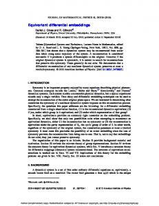
With this simple definition it turns out that the associated bisimulation equivalence, and others too, are congruences. But the family of all contexts is large and unwieldy. Can we make do with a subset of the contexts? Intuitively, we would like to have a transition a C . a0 only when C is “just large enough” so that Ca = Dl for some reaction rule (l; r) and context D. Then we would have a0 = Dr as the result of the transition. But what does “just large enough” mean? Suppose that C 0 a = D 0 l , i.e. the lefthand diagram in Figure 1 commutes. Informally speaking, C 0 may add more to a than is needed to create the redex l, i.e. C 0 may be larger than “just large enough”. A “smaller” context C may make the right-hand diagram of Figure 1 commute for some D and E . Then C is a more informative transition label than C 0 ; the transition a C . Dr tells us that Ca . Dr , hence also C 0 a . D 0 r 0 (because C 0 = EC and D 0 = ED ), which is what the transition a C . D 0 r would have told us. Example 1 (the � -calculus) Consider the asynchronous � -calculus [12], whose terms under structural congruence form a reactive system with the generic reaction rule
xhz i j x(y ):P
.
fz=ygP ;
i.e. the message z received on channel x replaces y in P . Let C 0 = [ ℄ j xhz i j z (w ):Q. Then 0 according to the definition (y) we would have the labelled transition x(y ):P C . fz=y gP j z (w ):Q. But we do not want this clumsy C 0 as a label in our LTS; it suffices to take the simpler context C = [ ℄ j xhz i, giving the transition
x(y ):P
C.
fz=ygP ;
which is a mere notational variant of the standard � -calculus transition this case D = [ ℄ and E = [ ℄ j z (w ):Q.
x(y ):P xhzi. fz=y gP . In
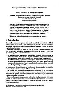
In general, given the first diagram in Figure 1, what is a minimal triple C; D; E making the second diagram commute? This minimality is made precise by Definition 46 in Section 10, which we reproduce here: Definition (relative pushout) In any category C, let fi ; hi (i = 0; 1) be arrows such that h0 f0 = h1 f1 (see Figure 2). A triple g0 ; g1 ; g is called a relative pushout (RPO) for f0 ; f1 wrt h0 ; h1 if 5
f0 f1
f0
h0
h1
f1
g00
g0 g1
h0 g g0
z g10
h1
Figure 2: A relative pushout g0 ; g1 ; g
g0 f0 = g1 f1 and ggi = hi , and moreover for any other triple g00 ; g10 ; g 0 such that g00 f0 = g10 f1 and g 0 gi0 = hi , there is an unique mediating arrow z such that zgi = gi0 and g 0 z = g . We shall often call a triple g00 ; g10 ; g 0 such that g00 f0 = g10 f1 and g 0 gi0 = hi a candidate; the definition makes clear the sense in which the RPO is the best candidate. An RPO, when it exists, is unique up to isomorphism; we therefore sometimes refer to the RPO. The relative pushout is a simple category-theoretic concept which may have a variety of applications (though we have not yet found the concept applied in the literature). RPOs have pleasant properties. When they exist, we may use the “just large enough” contexts C which they provide as the labels of an LTS. We showed in [17] that they yield sensibly modest label-sets; moreover, we proved that the associated bisimilarity and other equivalences are congruences.
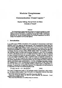
Action calculi reviewed We here review a restricted class of the action calculi which were presented in [20]. A closed, shallow action calculus is a strict monoidal category whose objects are integers k; `; m; n; : : : , and whose arrows are actions written a : (k; `), b : (m; n) etc. (We avoid the usual arrow notation a : k ! `, reserving it for the context arrows of reactive systems.) The tensor product of these two actions is a b : (k + m; ` + n); the composition of a : (k; `) and b : (`; m) is a � b : (k; m); the identity action of arity (m; m) is im . The order of composition is not conventional in category theory; we adopt it because it connotes the orientation of the action graphs we shall work with. We call (k; `) an arity and let �; ; : : : range over arities. In this paper we deal only with closed, shallow action calculi; we usually omit these adjectives from now on. A (closed, shallow) action calculus has a set of controls K; L; : : : , each with an arity. There are constants p : (2; 2), : (1; 2) and ! : (1; 0) for permutation, copy and discard. These constants represent only the swapping, sharing and elimination of arcs, not of nodes. They satisfy simple equations, e.g. � p = representing the commutativity of copying. There is also a trace operator in the sense of Joyal et al. [13], also known as reflexion, which we need not detail here. . , relating actions of equal arity. Finally, each action calculus has a binary reaction relation This relation is preserved by all constructions, i.e. by composition, tensor product and trace.
For examples of actions, let
K : (0; 1), M : (1; 1) and L : (1; 0) be controls. Then the following 6
K M
11 00 00 11 00 11
L
Figure 3: The action K � � (M
M M
L) and the context [ ; ℄ � � (M M ) 11
are actions, with their arities:
K M : (1; 2) K � � (M L) : (0; 1) (K � M ) (M � L) : (1; 1) :
We let “�” bind tighter than “ ”, so the last can be written K � M
M � L.
A context C is an action containing a single hole with arity �, written [� ℄. We omit the arity, writing [ ℄, if it is determined by the rest of the context or the surrounding discussion. Thus a context C : � ! is a term of arity with a hole of arity �. Here are two contexts with their source and target arities (the arity of the hole being fully determined in the second case):
[ ; ℄ � � (M M ) : (1; 1) ! (1; 2) K � [ ℄ � L : (1; 1) ! (0; 0) : 11
Figure 3 shows an action and a context using a graphical notation. It uses nodes (rectangles with two blunt corners) to represent occurrences of controls, and arcs to represent composition. An action or a hole with arity (m; n) has m source ports on its left side and n target ports on its right side. A control node of arity (m; n) has m target ports at its rectangular end and n source ports at its blunted end. At a source node, branching of arcs represents and absence of arcs represents ! . Two contexts are equal if the algebraic theory equates them, treating the hole as a control distinct from all others. The composition of two contexts C : � ! and D : ! , written here DÆ C (note the conventional order of composition), is formed by replacing the hole in D by C . Composition is clearly associative, and there is an identity context id� = [� ℄ for each arity. An action a : � can be considered as a context a : (0; 0) ! � whose hole has minimum arity. We shall use lower case letters a; : : : for actions. We have thus associated with an action calculus a reactive system ACxt0 , whose objects are arities, with distinguished null arity (0; 0), and whose arrows are contexts, including actions. The subscript 0 in ACxt0 refers to the closed shallow constraint.
3 Examples and a problem In this section we give examples of specific RPOs in ACxt0 , illustrating several phenomena. We end with an example showing cases in which RPOs fail to exist; this motivates the solution strategy of the ensuing section. 7
Remember that ACxt0 is really a family of reactive systems arising from action calculi; each is determined by a set of controls and a set of reaction rules. Example 2 (arithmetic) We first illustrate how a relative pushout can determine a labelled transition, using an action calculus for elementary arithmetic having controls 0, S and + with arities (0,1), (1,1) and (2,1). The reaction system is shown in Figure 4; it is an example of the sharing graphs of Hasegawa [10], which add sharing to the interaction nets of Lafont [15]. Nodes represent subexpressions, and the forking of arcs allows these to be shared. The reaction rules are in the top diagram; the garbage collection rules allow unattached expressions to be incrementally destroyed. The middle diagram shows an action (graph) a occurring in a larger one b0 , which also contains an occurrence of the redex l1 of the rule for S. The contexts C 0 and D 0 correspond to the two occurrences, which overlap. Now what is the “just large enough” context C which extends a to contain l1 ? It is not quite C 0 , because C 0 has destroyed the possibility of sharing S which is offered by l1 . In fact it is C as shown in the lower diagram; it may not seem “smaller” than C 0 , but it is indeed a factor of C 0 , as witnessed by the context E . (C 0 cannot be a factor of C ; no context F surrounding C 0 can cause its S-node to be shared.) So our derived labelled transition system will admit the transition a C . Dr1 . We would expect to add further controls, e.g. for subtraction, before obtaining an interesting behavioural congruence. Example 3 (wiring) The preceding example used the forking and deletion of arcs to represent the sharing of components. This non-linearity is a pervasive feature in practical systems. The � -calculus depends heavily on it; witness the double occurrence of x in its reaction rule shown in Example 1. Non-linearity can give rise to RPOs which are more complex than one might expect. Figure 5 shows two identical actions a = b = K � , where K : (0; 1); using the identity contexts C 0 = D0 = [0;2 ℄ they are embedded in K � . But the RPO C; D; E does not consist of identity contexts! A candidate might choose to identify t0 in a with either t2 or t3 in b, and similarly for t1 . To be the “best” candidate, the C; D; E must handle all these pairings; to indicate this we have indexed its targets by pairs in the diagram. In fact we have
Ca = Db = K � � ( ) : Example 4 (reflexion) A surprising phenomenon is how the presence of reflexion can affect the RPO. Let K; N : (1; 1), L : (0; 2) and M : (2; 0), and recall that i1 is the identity of arity (1; 1) for action composition. Figure 6 shows a = L � (i1 K ) and b = (i1 K ) � M embedded in C 0 a = D0 b = L�(N K )�M . The contexts C 0 and D0 do not involve reflexion. In the RPO C; D; E shown we have Ca = Db = (i1 L)�(p K )�(i1 M ); this extends a by only one control (M ) in order to create an occurrence of b. The contexts C and D do not use reflexion, but E does use it. If reflexion is forbidden then the RPO C + ; D + ; E + is such that C + a = D + b contains N ; this would yield a more complex transition label in the derived LTS. These examples do not exhaust the phenomena which arise in finding RPOs in ACxt0 , but they indicate that the general construction will not be trivial. The reader may feel that, having coped informally with a number of phenomena, we are well on the way to finding RPOs in every case. However, they do not always exist in ACxt0 ! Here is a counter-example. 8
l0
0
r0
0
0
+
S
l1
S
r1
S +
+
+
S
Arithmetic rules
Garbage collection rules
(1,1)
a
111 000
00 S 11 00 11 100 0 11 00 11 00 11
C0
+
b0 11111 00 000 S + 000 111 000 111
0
0
(1,1)
(0,0)
C 0 a = D 0 l1 = b 0
S +
00 00011 111 00 11 111 000 1 0 00 11 00 0 11
D0
l1 (2,2)
An action a overlapping a redex l1 (1,1)
a
11 S 00 100 0 11 00 11 00 11 00 11
(0,0)
11 00 111 000 1 0 00 11 111 000 1 0 00 11 00 0 11
C0
C
11 00 00 11 00 11 00 11 (1,2)
0
(1,1)
E D
l1
b S 1111 0 000 + 000 111 000 111 Ca = Dl1 = b
D0
(2,2) A relative pushout for a and l1 wrt C 0 and D 0 Figure 4: A reactive system for arithmetic (Example 2)
9
a
K
C K
(0,0)
K
11 00 00 11 00 11
11 00 00 11 00 11 00 11 E
t0 ;t2 ) t0 ;t3 ) t1 ;t2 ) (0,4) t1 ;t3 )
( ( ( (
D
b
11 C 0 00 00 11 00 11
(0,2)
t0 t1
t2 t3
11 00 00 11 00 11 00 11
0 1 1 0
(0,2)
K
(0,0)
(0,2)
11 00 00 11 00 D0 11
(0,2)
Figure 5: A relative pushout for copied wiring (Example 3)
L
a
110 00 1 N 00 11 00 11 111 00000 11 M
C0
(0,2) K
C L
(0,0)
11 00 00 11 00 11
K M
(1,1)
b
N
(0,0)
E
(0,0)
D N
K
M
(2,0)
0 1 1 0
L
011 1 00
00 11111 D0 000 00 11 L
Figure 6: A relative pushout using reflexion (Example 4)
10
N K
M
(0,0)
C0
(0,1)
a
K
K
L
11 00 L 00 11 00 11
(0,0)
b
(0,0)
K
K
D0
(0,1)
L
1 0
K
L
K
L
(0,0)
(0,0)
11 00 L 00 11 00 11
A context equation C 0 a = D 0 b (0,1) K �L [ ℄�L
[℄ [℄ K
K
C (0,0)
F0
K �L [ ℄�L
(0,0)
IMPOSSIBLE !
(0,0)
F1
D
(1,1) [ ℄ � (L L)
[℄
K
K [℄ K �L [ ℄�L
(0,1)
Figure 7: A missing relative pushout in ACxt0 (Example 5)
11
Example 5 (missing RPO) Let K : (0; 1) and L : (1; 0). Let a = b = K and let C 0 = D 0 = K � L [0;1 ℄ � L with arity (0; 1) ! (0; 0). Then C 0 a = D0 b = K � L K � L; this is shown in the upper diagram of Figure 7. The lower diagram shows two candidate RPOs, for which it is easy to verify commutation:
C0 ; D0 ; E0 = [ ℄; [ ℄ ; K �L [ ℄�L C1 ; D1 ; E1 = [ ℄ K ; K [ ℄ ; [ ℄ � (L L) : But if there were an RPO, then contexts C; D; F0 ; F1 would exist as shown making the diagram commute, yielding a contradiction as follows: Neither C nor D can contain any control, since F0 C = F0 D = [ ℄. Hence from CK = DK we deduce C = D, using the criterion for context equality stated above (since the control K appears in neither C nor D ). Hence [ ℄ K = F1 C = F1 D = K [ ℄, a contradiction. This counter-example involves neither copying nor discard of arcs, so it also denies the existence of all RPOs for linear action calculi – those in which all source ports bear exactly one arc. Thus we cannot attribute the lack of RPOs to and ! , even though they demand careful treatment as shown in Examples 2 and 3. The counter-example also illustrates why RPOs do not always exist in ACxt0 . The equations C0 K = D0 K = K and C1 K = D1 K = K K hold respectively for the two candidates; but if we “trail” the two occurrences of a = K and b = K through these equations, we find that they correspond to the same occurrence of K in the first case, and to two different occurrences in the second case. This is a key to solving our problem; we seek a reactive system which is a suitable refinement of ACxt0 , and which possesses the RPOs we need. We expect its contexts to represent trailing; in fact, it will be a version of the colouring used by Sewell [23] to get appropriate LTSs in certain classes of reactive system.
4 Solution strategy Our problem is how to use relative pushouts to derive, for an arbitrary action calculus, an LTS which yields behavioural congruence. Since we cannot find enough RPOs in the reactive system ACxt0 , we declared in the previous section that we would seek a refined version of it based upon trailing. The first task of this paper is, therefore, to define this refined reactive system, which we shall call PCxt0 . We then have two obligations. First, we have to show that from PCxt0 we can derive an LTS for ACxt0 whose associated behavioural equivalence is congruential. Second, which is the main topic of the paper, we have to prove that PCxt0 possesses enough RPOs. Here we explain in a little more detail how these two obligations will be tackled.
Deriving a labelled transition system We have already recalled from [17] the notion of RPO in an arbitrary category. A sister notion defined there is the following: 12
Definition (idem pushout) Let g0 f0 = g1 f1 in any category. Then (IPO) for f0 ; f1 if g0 ; g1 ; id is an RPO for f0 ; f1 .
g0 ; g1 is an idem pushout
In this case we may say that the equation g0 f0 = g1 f1 , or the corresponding commuting square, is an IPO. A given pair f0 ; f1 may have many IPOs; intuitively, each one is a a minimal upper bound, in contrast with a pushout which is the least upper bound for f0 ; f1 , up to isomorphism. In [17] IPOs were used to define an LTS as follows: Definition (labelled transition, first kind) Let a; a0 be actions and F a context in a reactive system A. Then there is a labelled transition a F . a0 iff there is a reaction rule (l; r ) and an IPO F a = Dl such that a0 = Dr. If RPOs (and hence IPOs) do not exist in A, can we nevertheless derive an LTS for A from another reactive system suitably related to A? A possible way is as follows: Definition (labelled transition, second kind) Let A be a reactive system and F : P ! A a functor. Let a; a0 be actions and F a context in A. Then there is a labelled transition a F . a0 iff there is a reaction rule (l; r ) and context D in A, and an IPO F^ a ^ = D^ ^l in P, such that F (F^ ) = F , 0 ^ ^ F (^a) = a, F (D) = D, F (l) = l and a = Dr. This is not enough in general; we cannot expect this definition to yield congruential behaviour relations for an arbitrary functor F , even if sufficient RPOs exist in P. But when A = ACxt0 , if we take P = PCxt0 (as we shall define it) then a functor F exists which does indeed achieve this important property. The definition of F , and a theorem to this effect, will be in Leifer’s forthcoming PhD Dissertation [16]. Briefly, PCxt0 arises by adding trailing to ACxt0 as follows. In contrast with a morphism in ACxt0
C : (m; n) ! (m0 ; n0 ) whose domain and codomain are arities, a morphism in PCxt0
C^ : (m; n; V ) ! (m0 ; n0 ; V 0 ) has as domain and codomain profiles of the form p = (m; n; V ) where V is a node set. The context C^ contains, in addition to the information contained in C , an injective map from V to V 0 identifying each node of an action (graph) a ^ with a node in the action (graph) C^ a^.
Establishing relative pushouts Our second obligation, and the focus of the present paper, is to demonstrate that enough RPOs exist in PCxt0 . We might try to work directly in PCxt0 , but it is much easier to work in an associated category GEmb0 , whose objects are action graphs and whose arrows are embeddings of one graph 13
in another. Just as ACxt0 is a functorial image of PCxt0 , so PCxt0 is a functorial image of GEmb0 . The analogy goes further, for the objects (graphs) of GEmb0 arise by adding information to the objects (profiles) of PCxt0 . If p = (m; n; V ) is a profile, then a graph G = (m; n; V; tr ; sr ) with profile p has also a function tr assigning a control to each node, and a function sr assigning a source port to each target port. Thus the overall picture has three levels:
Category
Objects
GEmb0 graphs Cod # PCxt0 profiles
F#
ACxt0
arities
Arrows
G = (m; n; V; tr ; sr ) p = (m; n; V ) � = (m; n)
embeddings
� : G ! G0
trailed contexts
C^ : p ! p0
contexts
C : � ! �0
The categories GEmb0 and PCxt0 are intimately related by a standard categorical notion; in fact GEmb0 is isomorphic to a coslice of PCxt0 . We shall in due course recall the notion of a coslice C0 of an arbitrary category C; it provides a simple codomain functor Cod between C0 and C, and enables us to reduce the existence of RPOs in C to the existence of simpler constructions, namely slice sums, in C0 . Thus, suppose that our first obligation is met by a suitable functor F . Then, to achieve behavioural congruence in ACxt0 , it is enough to establish the isomorphism mentioned above and then to construct slice sums in GEmb0 . The remainder of the paper is devoted to this task.
To keep the problem tractable we have chosen for this exercise to limit the contexts we admit in ACxt0 , and hence in PCxt0 . Instead of admitting the full power of reflexion in contexts, we exclude contexts which impose a reflexion on their “hole” without a mediating control node. The details are in Section 7. We have no reason to believe the results will not extend to permit these reflexions. However, for some purposes the limitation is irrelevant; for example in the normal representation of the � -calculus as an action calculus, the actions all have arity of the form (m; 0), for which reflexion is impossible. We take this matter up again in the concluding section. Outline The remainder of the paper is organized as follows. In Section 5 we define action graphs, with illustrations and nomeclature. In Section 6 we define the category GEmb0 of action graph embeddings; we characterize its isomorphisms, especially node renamings, and the subcategory GInc0 of inclusion embeddings. In Section 7 we introduce contexts. First we define PIns0 , the category of insertion contexts which correspond to inclusion embeddings. This leads to the definition of PCxt0 , the category of trailed contexts. In Section 8 we develop the correspondence between the two main categories. After introducing coslice categories, we first define a functor between GInc0 and the coslice category �=PIns0 , where � = (0; 0; ;) is the empty profile. This leads directly to a functor C : GEmb0 ! �=PCxt0 from embeddings to a coslice category of contexts. We conclude the section by introducing functions EG0;G1 taking contexts C such that CG0 = G1 and yielding embeddings � : G0 ! G1. In Section 9 14
we employ the functions EG0 ;G1 to demonstrate that C , which is easily seen to be isomorphic on objects, is in fact an isomorphism of categories. Section 10 begins with the definition of RPOs and slice sums, and then observes that the RPOs we need in PCxt0 correspond to slice sums in �=PCxt0 , and so in GEmb0 via the isomorphism C . It is shown that these still do not exist in all cases in GEmb0 . A key condition, SLICE , is then defined; it is argued that, in realistic action calculi, the S LICE condition will hold in those cases where slice sums are needed to establish a behavioural congruence. The main result follows: that S LICE is necessary and sufficient for the existence of a slice sum. Thus the goal of the present paper is achieved. The proof of the last-mentioned result is given in outline here; the full proof will appear in Leifer’s forthcoming PhD Dissertation [16].
5 Closed shallow action graphs In this section, after introducing some notation, we define the class of action graphs that are the subject of this paper.
P
Notation We write [m℄ for the ordinal S number f0; 1; : : : ; m 1g. The disjoint sum i2I Xi of a family of sets is taken to be the set i2I (fig � Xi ). A particular case is when I = [n℄; then the disjoint sum may be written, without parentheses, as X0 + X1 + � � � + Xn 1 . Examples in the paper P take forms such as S = v2V Sv + [m℄ + [n℄, a ternary disjoint sum, the first summand of which is itself a disjoint sum; S has elements of the form (0; (v; s)) for each v 2 V and s 2 Sv , (1; i) for each i 2 [m℄, and (2; j ) for each j 2 [n℄.
We write X #Y to mean that the sets X and Y are disjoint. In this case we often write their union as X ℄ Y , to remind us that they are disjoint. This conventional notation is to be distinguished from a disjoint sum. In particular, (X1 ℄ X2 ) ℄ X3 = X1 ℄ (X2 ℄ X3 ) and will often be written without parentheses; on the other hand, the disjoint sums X1 + X2 + X3 , (X1 + X2 ) + X3 and X1 + (X2 + X3 ) are all distinct but in bijective correspondence. If f : X ! Z and g : Y ! Z are two functions with X #Y , we may write f ℄ g : X ℄ Y ! Z for their combination. We write f : X � Y , f : X � Y and f : X � Y for respectively injective, surjective and bijective functions, and f : X ,! Y for an injection which is an inclusion. We use “Æ” for function composition, IdX for the identity function on the set X , and ;X for the empty function from ; to X . We often omit all but the inner parentheses in a nested function application, writing for example f1 f0 (x) for f1 (f0 (x)). In a category we usually use juxtaposition for composition and idA for the identity on the object A.
Definition 1 (controls) We fix a set K of controls, equipped with an arity function ar : K ! N 2 . We use K; L; : : : to range over K. For ar (K ) = (m; n) we write K : (m; n); in this case we also def def define arin (K ) = m, arout (K ) = n.
15
Definition 2 (action graph) A (closed, shallow) action graph G = (m; n; V; tr ; sr ) comprises an arity (m; n), a set V of nodes, a control map tr : V ! K assigning a control in K to each node in V , and a source map sr : T ! S assigning a source (port) in S to each target (port) in T , where
P
�
the source set S = v2V [arout ( tr (v ))℄ + v 2 V and the input sources indexed by [m℄;
�
the target set T = v2V [arin ( tr (v ))℄+[n℄ comprises the argument targets for each v and the output targets indexed by [n℄ .
def
def
[m℄ comprises the binding sources for each
P
2V
Nomenclature We may write a graph as G = (V; tr ; sr ) : (m; n), or just G = (V; tr ; sr ) when the arity is understood. We denote the empty graph (;; ;; ;) : (0; 0) by 0. We shall abbreviate arin ( tr (v )) to arin (v ) etc, when there is no ambiguity. We denote the injections induced by the disjoint sums S and T as follows:
bind (v ) : [arout (v )℄ � S in : [m℄ � S arg (v ) : [arin (v )℄ � T out : [n℄ � T
for the binding sources of each v 2 V ; for the input sources; for the argument targets of each v 2 V ; for the output targets.
We shall write bind (v; i) and arg (v; j ) for the ports bind (v )(i) and arg (v )(j ). For any injection f into a set A we write Af for the range of f ; thus for example S in is the set of all input sources and U arg (v) bind T the set of argument targets of v . We shall also write for example S for v2V S bind (v) . With this notation we can represent our partitions as
S = S in ℄ S bind T = T out ℄ T arg : An example of an action graph with arity (1; 3) is shown in Figure 8, with node names and the control map omitted. The whole graph is in a rectangle, with input sources at the left and output targets at the right. Nodes are drawn as rectangles with two corners blunted to give orientation; we may want to tilt some of them, as here, or even turn them upside down. The three nodes have arities (1; 1), (2; 1) and (1; 2). The arcs represent the source map, with arrows pointing from source to target. Ports could be drawn as blobs, but this is somewhat redundant; a target is always indicated by exactly one incoming arc, and we indicate a source with no outgoing arcs by a little aborted arc. Cycles are not prohibited. The graphs studied here are for action calculi which are closed, meaning that free names such as x; y; : : : are not used as sources, and shallow, meaning that control terms do not contain actions. This paper emphasizes the graphical rather than the algebraic aspects of action calculi. We study the closed, shallow graphs as a preliminary to the full graphical presentation of action calculi, since notions such as graph embedding and graph context are more clearly grasped in this simpler setting. From now on we shall usually omit the adjectives “closed” and “shallow”, understanding them to qualify all graphs throughout the paper.
16
Figure 8: A closed shallow action graph Convention Our graphs will almost always be denoted by G suitably subscripted. We shall not always explicitly list all their primary components V , tr , and sr , or their derived components S , T , bind , in etc; we shall follow a firm convention that the names of these components are standard, subscripted as necessary to connote the graph’s name.
6 Embeddings We now define the category GEmb0 in which the objects are graphs and the arrows are embeddings. Our main task is to define what we mean by graph embedding and to capture the meaning in a tractable list of axioms. Our approach differs from the standard approach to graph embedding due to Ehrig [5]; this point is taken up in the concluding section. Intuition Two graphs are shown in Figure 9. G0 is the graph of Figure 8, and G is a smaller graph which intuitively “occurs” in G0 . The way it occurs is represented informally by the dotted rectangle. The node v of G is represented by v 0 in G0 ; the input sources s0 and s1 are represented respectively by s00 and s01 , and the binding source s2 by s02 . The argument targets t0 and t1 are represented respectively by t00 and t01 , and the output target t2 by both t02 and t002 . The other output target of G is not represented in G0 ; the aborted arc (not formally part of G0 ) indicates that the lower arc from s2 in G is discarded by the embedding into G0 . Of course several parts of G0 don’t represent G. Also our definition of embedding must allow that a target of G may have any number (including 0) of representatives in G0 ; but we shall insist that every source in G is represented exactly once in G0 . Two sources may have the same representative, though this is not the case in our example. We are therefore led to the following definition: 17
s00
v0
t00 s1
t02
t002
s2 0
0
t01
G0 G
s0
t0
s1
t1
v
s2
t2
Figure 9: An embedding Definition 3 (embedding) For Gi = (Vi ; tr i ; sr i ) 2 GEmb0 , i = 0; 1, a (loose) embedding � : G0 ! G1 of G0 in G1 consists of a triple of functions (�V ; �S ; �T) where
�V : V0 � V1 is an injection of nodes; �S : S0 ! S1 is a map of sources; �T : T1 * T0 is a partial map of targets satisfying the following axioms: E- CTR E- SRC E- BIND E- ARG E- TARGS
: tr �V (v) = tr (v) : �S sr �T � sr : �S fbind (�V (v); i)g = fbind (v; i)g : �T farg (v; j )g = farg (�V (v); j )g : sr �S (S bind ) � Dom(�T) : 1
0
Æ
1
0Æ
1
1
1
1
1
0
0
1
0
These axioms deserve a little explanation. E- CTR says that � respects the control function; E- SRC says that it also respects the source function where �T is defined. E- BIND says not only that � respects the binding source functions, but also that �S never identifies (in G1 ) a binding source of G0 with any other source. This enforces the looseness constraint (see below). E- ARG is similar. E- TARGS says that if a source s in G1 represents a bound source of G0 , then all its targets represent targets of G0 . 18
The looseness constraint prevents an embedding where G1 creates a tight loop (such as is formed by the reflexion operator in action calculi) from the back of the G0 to the front. It does not preclude such a loop proceeding via a control, which indeed occurs in Figure 9; thus our embeddings will permit some but not all of the power of reflexion. To match full reflexion is more difficult and is not attempted here. This limitation on embeddings corresponds to the limitation on contexts mentioned in Section 4. We shall usually omit the adjective “loose” in this paper, as it applies to embeddings throughout. Proposition 4 An equivalent set of axioms is gained by replacing E- TARGS by the following: E- TARGS0 : If s0
2 S bind and �S(s ) = sr (t ) then �T(t ) is defined and s = sr �T(t ). 0
0
1
1
1
0
0
1
Proof It is clear that E- TARGS0 implies E- TARGS ; it remains to show that the given axioms imply def E- TARGS0 . Assume its antecedent. Since s0 2 S0bind , by E- TARGS t0 = �T (t1 ) is defined and therefore by E- SRC
�S sr 0 (t0 ) = sr 1 (t1 ) ;
= bind (v ; i) for some v , whence from E- BIND we have sr (t ) = �S (s ) = bind (�V (v ); i) : But E- BIND asserts that bind (�V (v ); i) has an unique preimage under �S , hence s = sr (t ) as also s0
0
0
0
1
1
1
0
1
0
0
0
0
0
required. Definition 5 (the category of graphs and embeddings) The objects of the category GEmb0 of (closed, shallow) graphs and (loose) embeddings are the graphs defined in Definition 2. The arrows are the embeddings defined in Definition 3. If � : G ! G0 and : G0 ! G00 are two embeddings, then their composition � : G ! G00 is defined by
� def =( The identity embedding idG
V
Æ
�V ;
S
Æ
� S ; �T
T
Æ
):
: G ! G is defined by idG
= (IdV ; IdS ; IdT ) :
def
This definition is justified by the following two propositions. Proposition 6 If �i
: Gi ! Gi
+1
are two embeddings (i = 0; 1), then �1 �0 is an embedding.
Proof It is clear that �V1 Æ �V0 is an injection, since its components are injections. It remains to show that �1 �0 satisfies the five axioms. The first four are stated in a form which makes the proof easy. Take E- BIND for example; we have
(�S �S) fbind ((�V �V )(v); i)g = �S �S fbind (�V �V (v); i)g = �S fbind (�V (v); i)g = fbind (v; i)g : 1Æ
0
1
2
1Æ
1
0
0
1
1
1
0
0
19
2
1
0
1
0
We now consider E- TARGS0 , which is easier to verify than E- TARGS . Assume the antecedent for �1 �0 , namely that
s0 2 S0bind and (�S1 �S0 )(s0 ) = sr 2 (t2 ) ; Æ
we must prove that (�T0 Æ �T1 )(t2 ) is defined and s0
= sr (�T �T)(t ). From the assumptions and E- BIND , we have s = �S (s ) 2 S bind and �S (s ) = 0Æ
0
2
1
def
1
E- TARGS0 for �1 it follows that
0
0
1
1
1
sr 2 (t2 ). By
t1 def = �T1 (t2 ) is defined and s1 = sr 1 (t1) : So we now have that s0
2 S bind and �S(s ) = sr (t ), which by E-TARGS0 for � 0
0
0
1
1
0
implies that
t0 def = �T0 (t1 ) is defined and s0 = sr 0 (t0) : These two properties yield the required result. Proposition 7 For all embeddings � : G ! G0 , � = � idG = idG0 �. For all embeddings �i : Gi ! Gi+1 (i = 0; 1; 2), (�2 �1 )�0 = �2 (�1 �0 ). The empty graph 0 is an initial object in GEmb0 . Proof Obvious from the form of the definitions. For any graph G we shall write 0G for the unique embedding 0 empty (partial) functions.
! G whose components are all
We now consider how to characterize the isomorphisms in GEmb0 , i.e. those embeddings � : G1 for which there exists � 1 : G1 ! G0 with � 1 � = idG0 and �� 1 = idG1 .
G0 !
Proposition 8 Let Gi = (Vi ; tr i ; sr i ) : (mi ; ni ) be two action graphs, i = 0; 1, and let �V : V0 � V1 , �S : S0 ! S1 and �T : T1 * T0 be three maps. Then � = (�V ; �S ; �T ) : G0 ! G1 is an isomorphism in GEmb0 iff its components are bijections satisfying I- CTR I- SRC I- BIND I- ARG
: tr �V = tr : �S sr �T = sr : �S bind (v) = bind �V (v) : �T arg �V (v) = arg (v) : 1Æ
Æ
0
0Æ
Æ
Æ
1
0
1
1
0
Proof (=)) First, the components have to be bijections in order that an inverse
� 1 = (�V 1 ; �S 1 ; �T 1 ) may exist. Second, the four conditions follow immediately from the first four embedding axioms. ((=) Since the components are bijections, the embedding axioms are deducible from the four given conditions; in particular, E- TARGS follows since �T is total. Hence � is an embedding. Now 20
define � 1 as above. It is clear that both �� 1 and � 1 � are identity embeddings, by the definition of composition; it only remains to show that � 1 is indeed an embedding. But we know its components are bijections, and hence from I- CTR , I- SRC , I- BIND and I- ARG we can readily deduce the same four properties for � 1 with subscripts 0; 1 interchanged. Hence, as for �, � 1 is an embedding and the proof is complete. Corollary 9 If � : G0 ! G1 is an isomorphism with Gi : (mi ; ni ), then m0 = m1 (= m say) and n0 = n1 (= n say), and there exist unique permutations � in : [m℄ ! [m℄ and � out : [n℄ ! [n℄ such that
in 1 Æ � in
= �S
Æ
in 0 and
�T out 1 = out 0 � out Æ
Æ
1
:
Proof With the notation of the proposition, we deduce from I- BIND that �S (S0bind ) = S1bind ; as �S is a bijection it follows that �S (S0in ) = S1in , whence immediately m0 = m1 . Then we may define � in (i) def = in 1 1 �S in 0(i), thus uniquely achieving the required condition. A similar argument applies for output targets. Definition 10 (profiles, permutations and node renamings) We call a triple (m; n; V ) (an arity and a node set) a profile. We call a pair � = (� in ; � out ) of bijections � in : [m℄ � [m℄ and � out : [n℄ � [n℄ an (arity) permutation (on m; n), and an injection � : U � U 0 , where V � U , a node renaming (on V ). We have shown, then, that each isomorphism of GEmb0 induces a permutation and a node renaming. We now wish to show that the converse is true, in a strong sense: Proposition 11 Let G : (m; n) have node set V . Let � be a permutation on m; n and � a node renaming on V . Then there exists a unique pair G0 ; � such that � : G ! G0 is an isomorphism in GEmb0 satisfying
�V = � � V : V = in 0 �in �T out 0 = out � out �S Æ in
�
V0
Æ
Æ
Æ
1
where in 0 ; out 0 are the input source and output target injections associated with G0 . Proof (outline) Let G0
= (V 0; tr 0; sr 0 ) : (m; n) and � : G ! G0 be defined as follows:
def
V 0 def = �V
tr 0 sr 0
= tr �V = �S sr �T �V = �(� V in 0 (� in (i)) �S (s) = 0 �(v ); k) (bind (out out (� (i)) �T (t) = arg (v; k) def
def
1
Æ
Æ
Æ
def
def
def
1
21
if s = in (i) if s = bind (v; k )
if t = out 0 (i) if t = arg 0 (�(v ); k )
The components of � are bijections satisfying the conditions in Proposition 8, hence � is an isomorphism; they also satisfy the present conditions required of �. It can be checked that any pair G0 ; � satisfying all these conditions will also satisfy the defining equations above. From now on we pay explicit attention to those isomorphisms which do not permute the arity. Definition 12 (node isomorphisms and actions) In the case that � = (Id[m℄ ; Id[n℄ ) is the identity permutation on m; n, we call the isomorphism � constructed in Proposition 11 a node isomorphism, and denote it just by �G . Furthermore, we denote the graph G0 for which �G : G ! G0 by
��G ; and we call the whole isomorphism, or sometimes � � G alone, the action of � upon G. When G is understood, we may write just � for the isomorphism �G . For future reference let us just record the components of this action. Proposition 13 Let G = (V; tr ; sr ) : (m; n) be a graph, and � be a node renaming on V . Then the components of � � G = (V 0 ; tr 0 ; sr 0 ) are related to those of G by the source and target components �S : S ! S 0 and �T : T 0 ! T of the isomorphism � : G ! � � G0 as follows:
V 0 = �V bind 0 �(v ) = �S bind (v ) in 0 = �S in
tr 0 � = tr �T arg 0 �(v ) = arg (v ) �T out 0 = out : sr 0 = �S sr �T Æ
Æ
Æ
Æ
Æ
Æ
Æ
Proof Already implicit in Proposition 11. We now consider those embeddings � : G ! G0 which preserve the names of the nodes of these will play an important role in the ensuing theory. Definition 14 (inclusions) An embedding �V : V ,! V 0 is an inclusion.
�: G
G;
! G0 is called an inclusion (embedding) if
It was pointed out after Definition 3 that for any embedding �, the restriction �S � S bind is an injection. This becomes an inclusion, when � is an inclusion embedding. A similar remark applies to the argument targets. Proposition 15 Every embedding � can be expressed uniquely as � = ��, with � an inclusion and � a node isomorphism. Proof Let � : G0 ! G1 . The node renaming � = �V : V0 � V1 yields by Proposition 13 the node def isomorphism � : G0 ! � � G0 , with �V = �V : V0 � �V0 . Define � : � � G0 ! G1 = �� 1 . 22
G0
�
G1 �G1
�G0 � � G0
���
� � G1
Figure 10: Action of a renaming upon an inclusion embedding Clearly � = ��, and � is seen to be an inclusion thus: each node of �V0 has the form v 0 = �V (v ), for some v 2 V0 ; so � V (v 0 ) = (�� 1 )V (�V (v )) = (�� 1 �)V (v ) = �V (v ) = v 0 . Moreover, it is straightforward to show that the requirement for � to be an inclusion determines � uniquely on V0 , hence determines � uniquely. It is clear that the identities are inclusions, and the composition of embeddings preserves the inclusion property. This justifies the following definition of a category we shall need later. Definition 16 (the category of graphs and inclusions) We define GInc0 to be the subcategory of GEmb0 having all the objects of GEmb0 , and as arrows just those embeddings which are inclusions. The category GInc0 contains no isomorphisms except those whose node component is the identity. As we have seen, node renamings � provide the opportunity to factor any embedding � as � = ��. But they have another role in relation to GInc0 ; we shall now define the quasi-functorial action of renamings upon GInc0 . Definition 17 (node renamings on inclusions) Let � : G0 and � a node renaming on V1 . Then the action of � upon � is
!G
1
be an inclusion embedding
� � � : � � G0 ! � � G1 ; defined by � � �
= �G1 ��G0 .
def
1
Proposition 18 The embedding � � � is an inclusion. Moreover it preserves identities and composition, i.e. � � id = id and � � (�1 �0 ) = (� � �1 )(� � �0 ) whenever the action is defined. Hence � � ( ) is a functor upon the full subcategory of GInc0 whose objects (graphs) have a node set included in Dom(�). Also the diagram in Figure 10 commutes, and thus the unique decomposition of an embedding of the form �G1 � is given by �G1 � = (� � � )�G0 . Proof Straightforward.
23
7 Contexts We shall now proceed to construct the category PCxt0 of closed shallow loose contexts, which will have a close correspondence with the embeddings category GEmb0 . The intuition of “context” is well supplied by Figure 9; the graph G occurs inside the dotted rectangle in G0 , and we may think of the context in which G is placed as that part of G0 lying outside the dotted rectangle. A context is therefore an action graph, but with a little more structure since it has an internal as well as an external interface. The internal interface is often called a hole. (We do not here consider contexts with more than one hole.) The upper diagram in Figure 11 shows an important variation of the embedding shown in Figure 9. The larger graph G0 is unchanged, but G now contains an arc which is pure “wiring”, not attached to any control node. Action graphs admit such possibilities, so our notion of context must allow for them. (In the extreme case either a graph or a context may have no nodes but consist only of wiring.) Note in particular that the sources s1 and s3 in G are both represented by s01 in G0 , and that t03 in G0 (which represented no target of the old G) represents the target t3 of the new G.
The lower diagram shows the context C which results when G is excised from G0 ; in the notation of what follows, G0 = CG (C composed with G). Note the new targets and sources on respectively the left and right sides of C ’s internal interface; in particular, the middle internal source lacks any targets and therefore represents the discard of the corresponding output target of G – or of any other graph – when placed in the hole. There are two stages in the contruction of PCxt0 . The first stage is to define the category PIns0 of shallow closed “insertion contexts”. They will correspond to inclusion embeddings; in PIns0 we shall allow composition of insertions only when they have disjoint node sets. Definition 19 (insertion contexts) A (closed, shallow, loose) insertion context A = (V; tr ; sr ) of arity (m0 ; n0 ) to (m; n), written A : (m0 ; n0 ) ! (m; n), comprises a set V of nodes, a control map tr : V ! K assigning a control in K to each node in V , and a source map sr : T ! S assigning a source (port) in S to each target (port) in T , where
P
�
0 the source set S = v2V [arout (v )℄ + [m℄ + [n ℄ comprises the binding sources for each v 2 V , the input sources indexed by [m℄, and the upput sources indexed by [n0 ℄;
�
0 the target set T = v2V [arin (v )℄ + [n℄ + [m ℄ comprises the argument targets for each v 2 V , the output targets indexed by [n℄, and the downput targets indexed by [m0 ℄.
def
def
P
Furthermore the looseness condition must be satisfied (see nomenclature defined below): L OOSE
:
sr (T down ) \ S up
=;:
We shall often call an insertion context an insertion. Note that an action graph G is just an insertion context A as above in which m0 = n0 = 0.
24
s00
t02
t00 s01
s2
t01
t03
G0 G
s0
t0
s1
t1
t002
0
s2
s3
t2
t3
Another embedding
111111 000000 000000 111111 000000 111111 000000 111111 000000 111111 000000 111111 000000 111111 000000 111111 000000 111111 000000 111111 000000 111111
The corresponding context Figure 11: An embedding and its associated action context
25
A1 S1in T1down
A0 0000 1111 0000 1111 T0down S0up 0000 1111 0000 1111 0000 1111 S0in 0000 1111
T1out T0out S1up
Figure 12: The composition of two insertions
The looseness condition, which was mentioned in Section 4, precludes a “tight” loop from the back of the hole to the front, such as is formed by the trace operator in action calculi. It does not preclude such a loop proceeding via a control, which indeed occurs in Figure 11; thus, just as with embeddings, our contexts permit only limited power of reflexion. We shall have to ensure that all contexts which we create – e.g. by composition – satisfy L OOSE . We shall continue to omit the adjectives “closed”, “shallow” and “loose” in this paper. Nomenclature
As for action graphs, there are induced injections for an insertion as follows:
bind (v ) : [arout (v )℄ � S in : [m℄ � S up : [n0 ℄ � S arg (v ) : [arin (v )℄ � T out : [n℄ � T down : [m0 ℄ � T
for the binding sources of each v 2 V ; for the input sources; for the upput sources; for the argument targets of each v 2 V ; for the output targets; for the downput targets.
With naming similar to that in action graphs for the partitions of S and T , we have
S = S bind ℄ S in ℄ S up T = T arg ℄ T out ℄ T down :
Definition 20 (The category of insertions) The category PIns0 of insertions has as objects prodef files of the form p = (m; n; U ), where U is a set. The profile � = (0; 0; ;) is called the empty profile. PIns0 has arrows A : (m0 ; n0 ; U 0 ) ! (m; n; U ), where U 0 � U and the insertion context A has node-set U n U 0 .
= (;; ;K; sr ) has � down (i) 7! in (i); i 2 [m℄ S = ; + [m℄ + [n℄ = S in ℄ S up sr : out down out (j ) 7! up (j ); j 2 [n℄ : T = ; + [n℄ + [m℄ = T ℄ T Now let Ai = (Vi ; tr i ; sr i ) : pi ! pi be two insertions, where pi = (mi ; ni ; Ui ) (i = 0; 1). The identity insertion idm;n;U
+1
Their composition, illustrated in Figure 12 by nesting A0 inside A1 , is
A1 � A0 def = A2 = (V2; tr 2 ; sr 2) : p0 ! p2 ; 26
= V ℄ V and tr = tr ℄ tr (thus determining ar = ar ℄ ar etc), and P [arout (v)℄ + [m ℄ + [n ℄ = (S bind ℄ S bind ) ℄ S in ℄ S up S = v2V2 P arg T = ℄ T arg ) ℄ T out ℄ T down : v2V2 [arin (v )℄ + [n ℄ + [m ℄ = (T Note (see Figure 12) that T down is in bijection with S in and [m ℄, while S up is in bijection with T out and [n ℄. It remains to define the source function sr ; this is done in terms of two auxiliary functions �i : Si ! S (i = 0; 1) which describe how sources of A and A “become” sources of where V2
def
def
1
0
2
1
0
2
1
0
def
2
2
2
def
2
2
2
0
0
1
0
A2 :
1
0
1
0
0
1
1
0
1
1
0
1
2
2
0
�0 (s) =
def
�1 (s) =
def
sr 2 (t)
=
def
� � �
s
sr 1 down 1 (i)
1
if s 2 S0bind ℄ S0up if s = in 0 (i) 2 S0in
s if s 2 S1bind ℄ S1in �0 sr 0 out 0 (j ) if s = up 1 (j ) 2 S1up �1 sr 1 (t) if t 2 T1arg ℄ T1out �0 sr 0 (t) if t 2 T0arg ℄ T0down :
We have adopted the symbol “ � ” for composition in PIns0 , as a reminder that the node sets of two insertions composed in this category are always disjoint. We earlier observed that an action graph G is just an insertion context whose hole has arity (m0 ; n0 ) = (0; 0). If G has node set V , we may now identify it with the arrow G : � ! (m; n; V ) of PIns0 . The above definition of PIns0 is justified by two propositions. Proposition 21 If A0 and A1 satisfy L OOSE , then so does A2
= A �A . 1
0
Proof We require t 2 T0down =) sr 2 (t) 62 S0up . We have sr 2 (t) = �0 sr 0 (t), and we consider cases for sr 0 (t). By L OOSE for A0 it cannot be in S0up . There are two other cases: Case sr 0 (t) 2 S0bind . Then sr 2 (t) = sr 0 (t) 2 S0bind .
Case sr 0 (t) = in 0 (i) 2 S0in . Then sr 2 (t) = sr 1 (t1 ) where t1 L OOSE for A1 we have sr 2 (t) 2 S1bind ℄ S1in .
= down (i) 2 T down , whence by 1
1
Proposition 22 For any A, id � A = A = A � id0 , where id0 and id are identities on the domain and codomain of A. Also composition is associative, i.e. for appropriately matching profiles A2 � (A1 � A0 ) = (A2 � A1 ) � A0 . Proof (Outline) The identity properties are easy to establish. For the associativity of composition, let Ai = (Vi ; tr i ; sr i ) : pi ! pi+1 , for i = 0; 1; 2, where pi = (mi ; ni ; Ui ). Using L and R to stand for left- and right- association, let
AL def = (A2 � A1 ) � A0 = (VL; tr L; sr L) def AR = A2 � (A1 � A0 ) = (VR ; tr R ; sr R ) : 27
Then it is easy to verify that
VL = VR = V2 ℄ V1 ℄ V0
tr L
= tr R =
tr 2 ℄ tr 1 ℄ tr 0
Hence AL and AR have the same arity function ar
2
= VL = VR , and
where V
P Pv2V [arout (v)℄ + [m ℄ + [n ℄
SL = SR = TL = TR = It remains to prove that sr L
:V !N
:
3
0
v2V [arin (v )℄ + [n ℄ + [m ℄ : 3
0
= sr R ; the detailed case analysis is in the Appendix.
Node renamings were defined in Definition 10, their action upon graphs in Definition 12, and their action upon inclusions in Definition 17. To prepare for the definition of PCxt0 we now define how they act upon insertions. Definition 23 (node renaming) A node renaming � on U determines an action profiles and insertions, as follows. Upon profiles, assuming V � U :
� � ( ) upon
� � (m; n; V ) def = (m; n; �V ) : Upon insertions, let A = (V; tr ; sr ) :
p0 ! p1 , with pi = (mi ; ni ; Ui ) and Ui � U ; then
� � A def = A 0 : � � p0 ! � � p1 where A0
= (V 0 ; tr 0 ; sr 0) is as follows: V0
tr 0 (�v ) S0 T0 sr 0
= �V = tr (v); thus determining ar 0 etc P = v2V 0 [arout 0(v)℄ + [m ℄ + [n ℄ P = v2V 0 [arin 0(v)℄ + [n ℄ + [m ℄
def def def
1
0
def
1
=
def
0
thus determining bijections �S �S Æ sr Æ �T :
: S � S 0 and �T : T 0 � T
Proposition 24 If A satisfies L OOSE then so does � � A. Proof Immediate from sr 0 output targets respectively.
= �S
def
Æ
sr Æ �T , since �S and �T are the identity on input sources and
Note in particular that � � A is only defined when the codomain of A is a subset of the domain of �. For what follows we need a few properties of node renamings:
28
Proposition 25 Node renamings satisfy the following, whenever they are defined:
(1) (2) (3) (4) (5)
� � (idm;n;U ) = idm;n;�U � � (A1 � A0 ) = � � A1 � � � A0 Id � A = A (�0 �) � A = �0 � (� � A) � � A = �0 � A if A has node set V and � � V = �0 � V : Æ
Thus, in particular, each node renaming with domain U is a functor on the full subcategory of PIns0 containing those objects whose node sets are subsets of U . We are now ready for the main definition of this section. As mentioned in Section 4, we shall define a category PCxt0 of contexts which “trail” the nodes of a graph; this role is played by node renamings. The definition is followed immediately by a justifying proposition. Definition 26 (the category of contexts) The category PCxt0 of (closed, shallow, loose) contexts has profiles as objects, and its arrows – the contexts – take the form
(A; �) : (m0; n0 ; U 0) ! (m; n; U ) where � : U 0 � U is called a trail and A : (m0 ; n0 ; �U 0 ) ! (m; n; U ) is an insertion. The identity def contexts are idm;n;U = (idm;n;U ; IdU ), and the composition of two contexts Ci = (Ai ; �1 ) : pi ! pi+1 , for i = 0; 1, is defined as follows:
C1 C0 def = (A1 � �1 � A0 ; �1 �0 ) : Æ
Proposition 27 The identities of PCxt0 satisfy id C = C = C id0 for appropriate domain and codomain; moreover composition satisfies (C2 C1 ) C0 = C2 (C1 C0 ) . Proof For the first, let i = 0; 1; 2. Then: id C
= = = = = =
C = (A; �) : (m0 ; n0 ; U 0 ) ! (m; n; U ); for the second, let Ci = (Ai ; �i ),
(id; IdU ) (A; �) (id � IdU � A; IdU �) C (A � � � id; � IdU 0 ) (A; �) (id; Id0U ) C id0 :
(C C ) C = = = = = 2
1
0
Æ
Proposition 25(3) and identity in PIns0 Proposition 25(1) and identity in PIns0
Æ
(A � � � A ; � � ) (A ; � ) ((A � � � A ) � (� � ) � A ; (� � ) � ) (A � (� � A � (� � ) � A ); � (� � )) (A � � � (A � � � A ); � (� � )) C (C C ) : 2
2
2
2
2
2
1
2Æ
1
2
1
1
0
2Æ
1
2
2
2Æ
1
1
0
1
1
0
2Æ
0
0
29
2Æ
0
2Æ
1Æ
1 Æ
1Æ
0
0
0
Proposition 22 Proposition 25(2,4)
Recall that a graph G : (m; n) with node set V is essentially an insertion context G : � ! (m; n; V ) in PIns0 . The corresponding context in PCxt0 is
(G; ;V ) : � ! (m; n; V ) ; where ;V stands for the empty renaming with codomain V . When working in PCxt0 we shall often abbreviate (G; ;V ) to G.
8 Functors from embeddings to contexts At the end of the previous section we noticed that graphs (V; tr ; sr ) : (m; n) correspond to contexts � ! (m; n; V ). In this section and the next we show that this correspondence leads to an isomorphism of categories GEmb0 � = �=PCxt0 ; where �=PCxt0 is a coslice category of PCxt0 ; this is a simple general notion that we shall now recall. A consequence of this result is that slice sums in GEmb0 correspond naturally to relative pushouts in PCxt0 , which is crucial in deriving labelled transition systems. Definition 28 (coslice categories) Let C be a category and let coslice category C=C as the following category: Objects: arrows f
C be an object of C. Define the
: C ! C 0 of C with fixed domain C .
f : C ! C 0 and g : C 0 00 h : C ! C of C such that hf = g . Arrows: if
! C 00 are two objects, then arrows h : f ! g are arrows
Remark The categories C=C and C are naturally related by a functor Cod : C=C ! C mapping each object f : C ! C 0 to its codomain C 0 and each arrow h : f ! hf to itself. See the discussion in Section 4. The functor Cod is an example of a discrete cofibration.
'
To establish an isomorphism C : GEmb0 ! �=PCxt0 , we begin by defining an isomorphism ' A : GInc0 ! �=PIns0 . The definition of C will then be a straightforward modification of A. Definition 29 (functor on inclusions) The functor A : GInc0 ! �=PIns0 is defined on objects def by A(G) = G : � ! (m; n; V ), where G = (V; tr ; sr ) : (m; n). Now let � : G0 ! G1 be an inclusion. Suppose
Gi = (Vi ; tr i ; sr i ) : (mi ; ni ); i = 0; 1 with V0
� V . Then 1
A(�) = A = (VA; tr A; sr A) : A(G ) ! A(G ) def
0
30
1
where VA
= V nV
def
1
and tr A
0
SA def = def TA =
= tr � VA (thus determining ar A = ar � VA etc), and
def
1
1
P up bind in v2VA [arout A (v )℄ + [m ℄ + [n ℄ = SA ℄ S ℄ S P [arin (v)℄ + [n ℄ + [m ℄ = T arg ℄ T out ℄ T down : A A v2VA 1
1
0
1
0
1
1
1
Note that S1up and T1down are in bijection with T0out and S0in respectively. Finally we define sr A :
8� up (j ) > > < sr (t) sr A (t) = > :S
if � T (t) defined, i.e. � T t = out 0 (j ); j 2 [n0 ℄ if � T (t) undefined if t 2 TAarg ℄ T1out ; if t = down 1 (i) 2 T1down ; i 2 [m0 ℄ :
1
def
1
� in 0 (i)
�
We now justify this definition by three propositions. Proposition 30
A(�) satisfies LOOSE .
Proof From the definition of sr A , if t 2 T1down then sr A (t) 2 � S (S0in ) � SAbind Proposition 31 For every two inclusion embeddings G0 ! G1 Moreover for every graph G, A(idG ) = idG and A(0G ) = G . �0
℄ S in . 1
� ! G , A(� � ) = A(� ) � A(� ). 1
2
1 0
1
0
Proof (outline) The full proof is given in the Appendix. To show that A(idG ) = idG and that A(0G) = G is easy; recall that 0G is the unique embedding of the empty graph in G. To show that A(�1 �0 ) = A(�1 ) � A(�0 ) we have to set out the components of the left- and right-hand sides in detail. It then emerges that all components are clearly identical except the source functions; to prove that these agree is routine but requires a detailed case analysis. Combining the two propositions above gives the following corollary: Corollary 32 The construction A defines a functor GInc0
! �=PIns . 0
Proof Proposition 30 guarantees that the images of embeddings are indeed arrows of PIns0 , while Proposition 31 ensures the functoriality of the construction A. The one thing that we still have to check is that A is well-defined in the sense that for every inclusion � : G0 ! G1 , we have that A(�) : A(G0) ! A(G1); in other words, that A(�) � G0 = G1 . To prove this, we use the fact that A(0G ) = G. In fact we obviously have that 0G1 = � 0G0 ; By functoriality we then have that A(0G1 ) = A(�) � A(0G0 ). Thus we also have that G1 = A(�) � G0. It is immediately clear that, on objects, A is a bijection. To prove that it is in fact an isomorphism of categories we then have to show that it is full and faithful [18], in other words that for every two graphs G0 and G1 the function
AG ;G : 0
1
GInc0 (G0 ; G1 )
�
! �=PIns (A(G ); A(G )) 7 ! A(�) 0
31
0
1
�
G0
G1
G0 )
A(
A
��( ) � � G0
���
�)
A(
� � G1
G1 )
A(
��( ) � � A(G0 )
� � A(� )
� � A(G1 )
Figure 13: How the functor A treats a node renaming is a bijection. We leave this to the next section where we will make use of inverse functions DG0 ;G1 that we shall define later in this section. Before extending A to a functor on all embeddings, we have to show how it interacts with node renaming. The action of renaming on inclusions and on contexts was defined in Definitions 17 and 23 respectively. Figure 13 shows how these two actions are related by the functor A. This relationship is made precise by the following two propositions (recall that A is the identity on objects). Proposition 33 For any �
: G ! G , the context � � A(�) is an arrow � � G ! � � G 0
1
0
1
in �=PIns0 .
Proof This property is an immediate consequence of Proposition 25(2) as
� � A(� ) � � � G0 = � � (A(� ) � G0 ) = � � G1 : Proposition 34 The functor A preserves node renaming, i.e. A(� � � ) = � � A(� ) . Proof See the Appendix. It is straightforward, but lays out quite a lot of data. Definition 35 (functor on embeddings) The functor C : GEmb0 ! �=PCxt0 from embeddings to contexts is defined on objects, i.e. graphs, essentially as A is. That is
;V C (G) = � G;! (m; n; V ) ; where G = (V; tr ; sr ) : (m; n) : (
def
)
Let � = �� be the unique factorisation of an embedding � into an inclusion � and a node isomorphism �; then C is defined on the embedding � by
C (�) = (A(�); �V) : def
Fortunately we have already done almost all the work to ensure that: Proposition 36
C : GEmb ! �=PCxt 0
0
is a functor. 32
Proof It is easy to check that C takes identities to identities. To show that it preserves composition, let � = �1 �0 . Let �i = �i �i be the unique factorisations of �1 and �0 assured by Proposition 15. Then � = �1 �1 �0 �0 . But by Proposition 18 we have that �1 �0 = (�1 � �0 )�1 , where � � �0 is an inclusion. Thus we have the unique factorisation � = (�1 (�1 � �0 ))(�1 �0 ); it follows that
C (�) = (A(� (� � )); �V ) : 1
1
�
0
On the other hand
C (� )C (� ) = (A(� ); �V ) (A(� ); �V ) by definition of C = (A(� ) � �V A(� ); �V �V ) by definition of composition = (A(� ) � � A(� ); �V ) by Proposition 34 = (A(� ) � A(� � ); �V ) V = (A(� (� � )); � ) by Proposition 31 = C (�) : We are now left with showing that C is well defined, i.e., that for every � : G ! G , C (G ) = C (�)C (G ). To this purpose observe that if � : G ! G and has decomposition � = ��, then we 1
0
1
0
1
1
1
1
1
�
�
0
0
1
1
1Æ
0
�
1
1
0
�
0
0
0
0
0
have that 0 = � � 0 and thus that � � 0G0
1
1
1
= 0� � G0 ; hence the following diagram commutes: � � 0G0
0 = ��0
0G1
� � G0 � G1
We now have the following chain of equalities:
C (G ) = (G ; ;V ) = (A(0G ); ;V ) = (A(� (� 0G )); ;V ) = (A(�) � A(� 0G ); ;V ) = (A(�) � � A(0G ); ;V ) = (A(�) � �V A(0G ); �V ;V ) = (A(�) � �V G ; �V ;V ) = (A(�); �V )(G ; ;V ) = C (�)C (G ) 1
1
1
1
by Proposition 31 by commutativity of the diagram above by functoriality of A, Proposition 31 by Proposition 34
1
�
0
1
�
0
�
1
0
�
�
1
0
0
0
0
by Proposition 31 by definition of composition of contexts by definition of C .
0
0
0
From now on we shall say that � : G0 ! G1 in GEmb0 is over C : C (G0 ) ! C (G1 ) if C (�) = C . Similarly in GInc0 , � : G0 ! G1 is over A : A(G0 ) ! A(G1 ) if A(� ) = A.
We now turn to the full and faithfulness problem: Given a context C : C (G0 ) ! C (G1 ), show that there is a unique embedding � : G0 ! G1 such that C (�) = C . We begin with the simpler problem: Given an insertion A : A(G0 ) ! A(G1 ), show that there is a unique inclusion � : G0 ! G1 such that A(� ) = A. We shall achieve this by providing a function DG0 ;G1 which is shown in the next section to be inverse to AG0 ;G1 . 33
A S in
G0 T down S0in
T out
T0out S up
Figure 14: Applying an insertion context to a graph Definition 37 (inclusion from insertion) Let G0 and G1 be graphs. We define a function DG0 ;G1 �=PIns0 (A(G0 ); A(G1 )) ! GInc0 (G0 ; G1 ) from insertions to inclusion embeddings.
:
Let A : A(G0 ) ! A(G1 ) be an insertion, where Gi = (Vi ; tr i ; sr i ) : (mi ; ni ) for i = 0; 1. Recall that by definition G1 = A � G0 . Thus if A = (V; tr ; sr ) then the components of G1 = A � G0 = (V1; tr 1; sr 1) are as follows (a special case of insertion composition, see Figure 14):
℄V = tr ℄ tr = (S bind ℄ S bind ) ℄ S in = (T arg ℄ T arg ) ℄ T out and � (t) if t 2 T arg ℄ T out = �� sr sr (t) if t 2 T arg where � in (i) 2 S in = ssr down (i) ifif ss = 2 S bind � up (j ) 2 S up = �s sr out (j ) ifif ss = 2 S bind ℄ S in :
V1 = V
tr 1
S1 T1
sr 1 (t)
�0 (s) � (s)
0
0
0
0
0
0
0
0
0
0
0
0
The components of the inclusion embedding DG0 ;G1 (A) = �
:G !G 0
1
are then defined by
�V : V0 ,! V1 def = v 7! v (v 2 V0) def �S : S0 ! S1 = �0 8 if t 2 T0arg < �t � def �T : T1 * T0 = t 7! undefined if sr (t) 2 S bind ℄ S in : out 0(j ) if sr (t) = up (j ) 2 S up if t 2 T arg ℄ T out :
This definition is justified by Proposition 38
� = DG0 ;G1 (A) is an inclusion embedding. 34
Proof First, � V is an inclusion map, so it remains to check that the five embedding axioms hold. E- CTR is immediate. For E- BIND , first note that � S is well defined, i.e. �0 (s) 2 S1 for each s 2 S0 ; this is because, in the second case of �0 ’s definition, sr (down (i)) 2 S up is impossible by L OOSE for A. Then E- BIND follows noting that �0 (s) 2 S0bind iff s 2 S0bind . For E- ARG , note similarly that � T (t) 2 T0arg iff t 2 T0arg . For E- SRC , suppose � T (t) is defined. Case
t 2 T arg ℄ T out and sr (t) = up (j ) �S sr 0 �T (t).
2 S up :
Case
t 2 T0arg : then sr t (t) = �0 sr 0 (t) = �S sr 0 �T (t).
then sr 1 (t)
= � up (j ) = � sr 0
0
out (j )
=
For E- TARGS , we require that if � T (t) is undefined then sr 1 (t) 62 S0bind . If � T (t) is undefined then t 2 T arg ℄ T out and sr (t) 2 S bind ℄ S in . Hence sr 1 (t) 2 � (S bind ℄ S in ) = S bind ℄ S in , disjoint from S0bind . The last task of this section is to define a function EG0 ;G1 which we intend as an inverse for CG0 ;G1 , just as we intend DG0 ;G1 as an inverse for AG0 ;G1 . The actual proof that these are indeed inverses will be carried out in the next section. Definition 39 (embedding from context) The function EG0 ;G1 from contexts to embeddings is defined as follows. Let C = (A; �) be a context such that (G1 ; ;V1 ) = (A; �)(G0 ; ;V0 ). In other words C is an arrow C (G0 ) ! C (G1 ) in �=PCxt0 . Then, by definition, G1 = A � � � G0 . Moreover we also have � : G0 ! � � G0 , and D� � G0 ;G1 (A) : � � G0 ! G1 .We therefore define
EG ;G (C ) : G ! G = D� G ;G (A) � : def
0
0
1
1
�
0
1
Thus E is built from D , just as C is built from A.
9 Functor inverses In this section we demonstrate that the function
CG ;G : GEmb (G ; G ) ! �=PCxt (C (G ); C (G )) 0
1
0
0
1
0
0
1
and the function
EG ;G : �=PCxt (C (G ); C (G )) ! GEmb (G ; G ) are inverses of each other. This implies that CG ;G is a bijection and thus that C is an isomorphism of categories. This main result depends upon the analogous property that the function AG ;G and the function DG ;G invert one another. We prove the latter first. 0
1
0
0
1
0
0
0
1
1
0
0
1
35
1
For the remainder of this section, when no confusion arises, we will omit for readability the subscript G0 ; G1 from CG0 ;G1 , EG0 ;G1 , AG0 ;G1 and DG0 ;G1 . Proposition 40 Let A :
A(G ) ! A(G ) be an insertion context. Then A(D(A)) = A. 0
1
Proof First we construct � = D (A) : of A, Definition 29, to give us
G0 ! G1 as in Definition 37. We now apply the definition
A0 = A(�) = (V 0 ; tr 0 ; sr 0 ) : A(G0 ) ! A(G1 ) whose first two components are readily found to agree with those of A. Furthermore:
S0 = S = T0 = T =
P [arout (v)℄ + [m ℄ + [n ℄ = S bind ℄ S in ℄ S up Pv2V arg ℄ T out ℄ T down : v2V [arin (v )℄ + [n ℄ + [m ℄ = T 1
0
1
0
We also have the source function of A0 :
8� up (j ) > > < sr (t) sr 0 (t) = > :S def
1
� in 0 (i)
It therefore remains to prove that sr 0 Case
t
sr 0 (t)
Then by definition
def
def
�
= sr . There are three cases:
2 T arg ℄ T out and sr (t) 2 S bind ℄ S in .
= � sr (t) = sr (t). Case t 2 T arg ℄ T out and sr (t) = sr 0 (t) = up (j ) = sr (t). Case
if � T (t) defined, i.e. � T t = out 0 (j ); j 2 [n0 ℄ if � T (t) undefined if t 2 T arg ℄ T out ; if t = down (i) 2 T down ; i 2 [m0 ℄ :
up (j )
2 S up .
�T (t) is undefined, hence
Then by definition
�T (t) = out 0 (j ), hence
t = down (i) 2 T down . Then sr 0 (t) def = �S in 0(i) = �0 in 0(i) = sr down (i) = sr (t).
This concludes the proof that A0 Proposition 41 Let �
:G !G 0
= A, and hence that A(D(A)) = A. 1
be an inclusion embedding. Then D (A(� )) = � .
Proof The argument is somewhat detailed and can be found in the Appendix. Proposition 40 and Proposition 41 say that D is both a left and a right inverse for A, and thus that A is full and faithful.. Since, as we said earlier, A is a bijection on objects, this is enough to conclude the following: Proposition 42 The functor A : GInc0
! �=PIns
0
36
is an isomorphism of categories.
We shall now complete the work of the section by lifting the foregoing results to full embeddings and full contexts. Proposition 43 Let C Proof Let C
: C (G ) ! C (G ) be an arbitrary context. Then C (E (C )) = C . 0
1
= (A; �) and � = E (C ). Then � = � � where � = D� � G0 ; G1 (A) and � = �V . Hence
C (E (C )) = C (� �) = (A(�); �V ) = (A; �V ) = (A; �) = C:
Proposition 44 Let � :
by definition of C by Proposition 40
G0 ! G1 be an arbitrary embedding. Then E (C (�)) = �.
Proof Let the unique factorisation of � into an inclusion and a node renaming be � � : V0 � V1 = �V . Then C (�) = (A(� ); �) by definition. So
E (C (�)) = D� G ; G (A(�)) � = �� = �:
�
0
1
= � �, where
by definition by Proposition 41
Finally, exactly as we did for A, we deduce that Theorem 45 The functor C : GEmb0
! �=PCxt
0
is an isomorphism of categories.
10 Relative pushouts for contexts The last section concluded by stating that the category of graphs and graph embeddings GEmb0 is isomorphic to the coslice category �=PCxt0 . In this section we use this result to show that PCxt0 possesses enough RPOs to ensure that a wide class of LTSs derived for action calculi will yield behavioural congruences. We shall first define RPOs and prove a few results about them. For this pure category theory we denote objects by A; B; C; : : : and arrows by f; g; h; : : : . When we come to apply the results we shall revert to our applied notation. Definition 46 (relative pushout) In any category C, let fi ; hi (i = 0; 1) be arrows such that h0 f0 = h1 f1 (see Figure 15). A triple g0 ; g1 ; g is called a relative pushout (RPO) for f0 ; f1 wrt h0 ; h1 if g0 f0 = g1 f1 and ggi = hi , and moreover for any other triple g00 ; g10 ; g 0 such that g00 f0 = g10 f1 and g 0 gi0 = hi , there is an unique mediating arrow z such that zgi = gi0 and g 0 z = g . 37
f0 f1
f0
h0
h1
g00
g0
g g0
z
g1
f1
h0
g10
h1
Figure 15: A relative pushout g0 ; g1 ; g
h0
g00
g0
h1
g1
h0 g g0
z g10
h1
Figure 16: A slice sum g0 ; g1 ; g
A closely related concept is the following: Definition 47 (slice sum) In any category C, let h0 ; h1 be a pair of arrows with a common codomain (see Figure 16). A triple g0 ; g1 ; g for which ggi = hi (i = 0; 1) is a slice sum of h0 ; h1 if, for any other triple g00 ; g10 ; g 0 such that ggi0 = h0i , there is an unique mediating arrow z such that zgi = gi0 and g 0 z = g . Remark RPOs and slice sums are pushouts and coproducts in slice categories (the obvious dual notion to that of coslice, cf. Definition 28). We make no specific use of this observation. Nomenclature If h0 ; h1 is a pair of arrows as in Figure 16, we call a triple g0 ; g1 ; g for which ggi = hi a candidate (slice sum) for h0 ; h1 . If C is an object of C, slice sums in the coslice category C=C correspond to RPOs in C for pairs of arrows with domain C : Proposition 48 Let C be a category. Let C; C0 ; C1 ; C2 be four objects of C, and fi : C ! Ci , hi : Ci ! C2 (i = 0; 1) four arrows of C. If we regard f0 and f1 as objects of C=C and hi : fi ! hi fi as arrows of C=C, respectively, the triple g0 ; g1 ; g is a slice sum of h0 ; h1 iff it is an RPO in C for f0 ; f1 wrt h0 ; h1 .
38
C (� ) 0
�0
G0
G
0
G2
G0
0
�
t t0
G1
1
G1
C( )
�1
C( ) 1
1 0 0 1 0 1
C( ) 1 0 0 1 0 1
1 0 0 1 0 1
1 0 0 1
1 0 0 1 0 C (�1 ) 1
Figure 17: A slice sum in GEmb0 becomes a relative pushout in PCxt0
Proof The proof is a trivial consequence of the definitions of slice sum and RPO applied to the categories C=C and C respectively. This proposition relates RPOs in PCxt0 to slice sums in (m; n; U )=PCxt0 . In particular we are interested in RPOs for pairs of contexts out of the empty profile � (actions), so we focus on slice sums in �=PCxt0 . As shown in the previous section, C : GEmb0 ! �=PCxt0 is an isomorphism of categories, so preserves slice sums. We shall use these facts in Corollary 57 to derive RPOs for PCxt0 from slice sums in GEmb0 . We now illustrate this derivation for a simple example in Figure 17. The left diagram shows a slice sum 0 ; 1 ; for �0 ; �1 in GEmb0 , which becomes an RPO in PCxt0 via C . (Recall that an arrow C (�) of �=PCxt0 is also an arrow of PCxt0 .) Note that C ( 0 ) G0 = C ( 1 ) G1 = G2 and C ( ) C ( i ) = C ( i ) = C (�), thus the proposed RPO commutes correctly. The source and target maps of 0 , 1 and are shown as dotted lines. For example the embedding of G0 ’s single arc into G2 is represented by the hole in the context C ( 0 ). Since G has no targets, the target map T is empty; this corresponds to the discarding of the targets t and t0 , represented by the aborted arcs in C ( ). Just as in the action b of Figure 4 in Example 2 (arithmetic), the extra arc of G2 connecting the control node to t0 may seem at first superfluous. But it is essential, since a competing candidate can have a target like t0 , sourced by the control node, that is mapped back to G1 but not to G0 . This distinguishes it from t, which is mapped to both. By E- TARGS there are no other possibilities (such as a target mapped to G0 but not to G1 ). Thus G2 contains precisely the targets it needs to be “as good as” any candidate. The formal construction of G2 is given later in Theorem 55. Our task now is to establish slice sums in GEmb0 . They are not always present! Figure 18 shows a case with no controls – only “wiring” – in which there is no slice sum. G0 is a graph with a single input source s0 and output target t0 , with s0 = sr 0 (t0 ); G1 is similar. G has a single source but no target. H and H 0 are candidate slice sums – one with a single arc and one with two sources 39
G0
t0
s0
�0 H G
69G
G1
2
H0 �1
t1
s1
Figure 18: A case where no slice sum exists and no arcs. The source and targets maps of the embeddings into H and H 0 are shown as dotted lines. These maps are not shown for embeddings into G (they are simple: all sources go to the single source in G, and G has no target to map). Now any slice sum G2 must possess embeddings from Gi and to H and H 0 as shown by dashed lines, making the diagram commute. But no such embeddings can exist. The reader may enjoy proving this. However, slice sums exist for many pairs of embeddings. We define below a condition S LICE , which characterises exactly these pairs, i.e., is a necessary and sufficient condition for the existence of slice sums. Details of the definitions and proofs which we outline in the remainder of this section will appear in Leifer’s forthcoming PhD Dissertation [16]; here we give the main definitions, and state the auxiliary results and main theorem with outlined proofs. First we define a key equivalence on which S LICE depends. Definition 49 (source coalescing) Let �i : Gi ! G (i = 0; 1) be a pair of embeddings. The source coalescing of �0 ; �1 is the smallest equivalence relation �� on S0 +S1 such that sr 0 �T0 (t) �� sr 1 �T1 (t) for all t 2 Dom �T0 \ Dom �T1 . An important property of �� is that it relates sources that must be equated in any candidate, as shown by the following proposition: Proposition 50 Let 0 ; 1 ; If s0 �� s1 then 0S (s0 ) =
be any candidate for �0 ; �1 and let si be a source of Gi for i = 0; 1. 1 (s1 ). S
Definition 51 (S LICE ) Let �i be as in the previous definition. The S LICE condition holds for 40
�0 ; �1 if for all si s0 �� s1 .
2 Siin and ti 2 Tiout (i = 0; 1), if si = sr i(ti) and �S(s ) = �S(s ) then 0
0
1
1
The reader may like to check that S LICE fails for the pair �0 ; �1 in Figure 18. The S LICE condition is implied by a striking property which is asymmetric between G0 and G1 : Definition 52 (output-controlled) In any graph, a target is controlled if its source is a bound source. G is output-controlled if all its output targets are controlled. Proposition 53 If satisfies S LICE .
G1 is output-controlled, then any pair of embeddings �i : Gi
! G (i = 0; 1)
Our interest in this fact arises because we are mainly concerned to find slice sums, or RPOs, when . can one of the graphs is a redex. In all cases we have met, the required reaction relation be achieved with reaction rules whose redexes are output-controlled. The reason appears to be as follows. Let (l; r ) be a reaction rule whose redex l in not output-controlled. Consider all arcs sr (t) = s in l where s is an input source and t an output target. If the contractum r possesses all these arcs, then it can be shown that the alternative rule (l0 ; r 0 ) with all such arcs removed yields exactly the same reactions; hence the rule can be replaced by (l0 ; r 0 ) for the purpose of deriving an LTS. If on the other hand r does not contain such an arc then the rule (l; r ) appears to generate non-deterministic behaviour of a kind not normally required. So it appears that if the argument below showing the existence of slice sums can be generalised to richer action calculi (deep, open, etc.) then congruential LTSs can be derived when we need them since the requirement that redexes are output-controlled is tolerable. We confine our argument to the category GInc0 of inclusions, returning to GEmb0 in Corollary 56. Let us fix a pair �i : G1 ! G (i = 0; 1) of inclusions. To show that S LICE is sufficient for �0 ; �1 to have a slice sum, we could give a direct construction. However, we also wish to show that S LICE is necessary, and therefore require a second candidate to argue that no slice sum exists when S LICE fails. To factor the work of constructing both candidates, we now give a general way to lift a triple of partial maps �0T ; �1T ; � T to a candidate �0 ; �1 ; � . Only those triples that satisfy certain conditions (omitted here) can be so lifted; we call them target scaffolds (for �0 ; �1 ). We first show how to make a candidate from a target scaffold. Then we prove S LICE ’s sufficiency by exhibiting a particular target scaffold �0T ; �1T ; � T , lifting it to a candidate, and, subject to S LICE , proving that this candidate is a slice sum. Finally we prove S LICE ’s necessity by exhibiting a second target scaffold, �^0T ; �^1T ; �^T , lifting it to a candidate, and showing that the negation of S LICE implies that no putative slice sum is better than both �; �0 ; �1 and �^; �^0 ; �^1 . Lemma 54 Every target scaffold for �0 ; �1 consisting of a set T2 and a triple of partial maps �0T; �1T ; � T, where � T : T * T2 and �iT : T2 * Ti , yields a graph G2 and a candidate �0 ; �1; � with � : G ! G2 and �i : G2 ! Gi .
41
Proof (sketch) We find it convenient to express our construction of G2 up to bijection of its source def and target sets, rather than in the exact form of Definition 2. Let G2 = (V2 ; tr 2 ; sr 2 ) : (m2 ; n2 ) where the parts are defined as follows. First we consider the vertices and targets of G2 :
= V [V
tr (v ) = tr (v) for v 2 V arg (v; k) = � Targ (v; k) for v 2 V n = jT j jIm arg j : V2
def
0
1
def
2
2
def
2
def
2
2
2
2
Notice that V0 and V1 are not necessarily disjoint: since �0V and �1V are inclusions, V0 [ V1 contains the vertices of G0 and G1 with appropriate overlap. Now we consider the sources and source maps. Take S0 + S1 satisfying the following conditions:
=: s for si 2 Sibind , s i 2 S i , and � S (s ) = � S (s ) =: sr � T(t) for t 2 Dom � T \ Dom � T :
s0 sr 0 �0T (t) Let [ ℄=:
=: to be the least equivalence relation on
1
1
1
1 1
0
0
0
1
1
1
: S + S ! (S + S )==: map sources to their equivalence classes. Then, let: 0
1
0
1
= bind (v; k) = m = sr (t) = �iS (s) = � S ([s℄ : ) = S2
def
def
2
def
2
def
2
def
def
=
(S + S )==: [bind i(v; k)℄ : 0
1
=
jS j jIm bind j 2
if v
2 Vi
2
[sr i�iT(t)℄ : if t 2 Dom �iT [s℄ : for s 2 Si for s 2 Si : �iS (s) =
=
From the conditions defining target scaffolds it can be verified that G2 is a graph, that �0 ; �1 ; � are all well-defined inclusion embeddings, and that together they form a candidate for �0 ; �1 . We now come to the main applied theorem of the paper. Theorem 55 A pair of inclusion embeddings �i : Gi ! G (i = 0; 1) satisfies S LICE if and only if there exists a triple �0 ; �1 ; � of inclusion embeddings forming a slice sum for �0 ; �1 in GInc0 . Proof (outline: for full details see Leifer [16]). Sufficiency: We exhibit a target scaffold consisting of a set
42
T2 and a triple �0T ; �1T ; �T , which we
lift to a slice sum. Let:
A + O0 + O0;1 + O1 farg (v; k) j v 2 V0 [ V1 g def f(t0 ; t1) 2 T0out � T1out j �0Ssr 0(t0 ) = �1Ssr 1(t1 )g def f8ti 2 Tiout j �iS sr i(ti) 2= �1S i (S1bindi )g > �iT (t) if t 2 A < �iT (t) def = >t if t 2 Oi :ti if t = (t0 ; t1 ) 2 O0;1 8 > if t 2 A T T : (�0 (t); �1 (t)) if t 2= A and t 2 Dom �0T \ Dom �1T . T2 A O0;1 Oi
= = = =
def
def
It can be verified that �0T ; �1T ; � T is a target scaffold, so can be lifted to a candidate �0 ; �1 ; � . We also claim that S LICE implies that �0 ; �1 ; � is a slice sum. At this point the reader may like to refer to the remark following the proof, which illustrates this construction with reference to examples. Necessity: Construct a second candidate for �0 ; �1 as follows. Let def T^2 = Dom �0T [ Dom �1T �^T : T * T^ def = t 7! t for t 2 T^ �^iT : T^ * Ti def = �iT�T^ :
Then �^0T ; �^1T ; �^T is a target scaffold, hence can be extended to a candidate �^0 ; �^1 ; �^. This candidate has a useful property which we state without proof: if si is an input source of Gi for i = 0; 1 then s0 6�� s1 implies �^0S (s0 ) 6= �^1S (s1 ).
Suppose that the S LICE condition does not hold, i.e. there are si 2 Siin and ti 2 Tiout such that sr i (ti ) = si , �0S (s0 ) = �1S (s1 ), and s0 6�� s1 . Suppose for contradiction that there is a graph G3 and a slice sum triple �0 ; �1 ; � such that � : G3 ! G and �i : Gi ! G3 for i = 0; 1. By the definition of slice sum, there exists mediating inclusions � : G3 ! G2 and � : G3 ! G^ 2 .
As observed above, s0 6�� s1 implies �^0S (s0 ) 6= �^1S (s1 ), hence � S �0S (s0 ) 6= � S �1S (s1 ), hence �0S(s0 ) 6= �1S (s1 ). However, (t0 ; t1 ) 2 O0;1 , so �iS (si ) = �iS sr i (ti ) = �iS sr i �iT (t0 ; t1 ) = �iSsr i �iT �T (t0 ; t1 ) = sr 3 �T (t0 ; t1 ) by I-SRC for �i; so �0S (s0 ) = �1S (s1 ), a contradiction.
Remark The construction of T2 in the first part of this proof appears complex, so the reader may wish to pattern-match it against the target sets of the RPO examples given in Section 3. As we will see shortly (Corollary 57) there is a tight correspondence: T2 is exactly the target set of an RPO action, as we now illustrate. 43
Example 2 (arithmetic): Consider the action graphs G0 = a and G1 = l1 in Figure 4, embedded in b0 . The targets of G2 = b, the RPO graph, correspond exactly to T2 ; in particular, the extra arc in b connecting S to the top output target is generated by the set O1 in the definition of T2 . Similarly, t0 2 O1 in Figure 17. Example 3 (wiring): Consider the identical action graphs G0 = a and G1 = b in Figure 5, embedded in an identical graph. The targets f(t0 ; t2 ); : : : ; (t1 ; t3 )g of K in G = Ca = Db are generated by the set O0;1 (a subset of the product of the targets from G0 and G1 ) in the definition of T2 .
Corollary 56 The embeddings �i : Gi ! G (i = 0; 1) satisfy property S LICE if and only if there exist a graph G2 and embeddings i : Gi ! G2 (i = 0; 1) and : G2 ! G forming a slice sum for �0 ; �1 in GEmb0 . Proof (outline) (=)) By Proposition 15 �i = �i �i (i = 0; 1), where �i is an isomorphism and �i an inclusion. The pair �0 ; �1 has property S LICE , since isomorphism does not disturb it; therefore, by Theorem 55, in GInc0 there is a slice sum �0 ; �1 ; � for �0 ; �1 . It is then not hard to show that �0 �0 ; �1 �1 ; � is a slice sum for �0 ; �1 in GEmb0 ; one needs the fact that if �0 and �0 � are inclusions then so is �.
((=) The argument can be essentially reversed. Let 0 ; 1 ; be a slice sum for �0 ; �1 in GEmb0 . def Let = �� , with � an inclusion and � an iso. Then setting �i = � i �i 1 , (i = 0; 1), we can show that �0 ; �1 ; � is a slice sum for the pair �0 ; �1 , which therefore has property S LICE . Hence also the pair �0 ; �1 has property S LICE . We are finally ready to deduce the existence of RPOs in the category PCxt0 of contexts, which is the goal set for the paper in Section 4. Recall that in PCxt0 a context C : � ! (m; n; V ), whose domain is the empty profile, is a pair (G; ;V ) consisting of a graph G with arity (m; n) and the empty renaming into V ; we abbreviate this pair to G. Corollary 57 Let C0 G0 = C1 G1 an RPO for G0 ; G1 wrt C0 ; C1 .
= G in PCxt , where G 0
1
is output-controlled. Then there exists
Proof Let �i = EGi ;G (Ci ), for i = 0; 1. Since G1 is output-controlled the pair �0 ; �1 satisfies property S LICE by Proposition 53, hence possesses a slice sum by Corollary 56. The isomorphism C : GEmb0 ! �=PCxt0 transforms any such slice sum into a slice sum of C0 : C (G0) ! C (G) and C1 : C (G1 ) ! C (G), and hence, by Proposition 48, into an RPO in PCxt0 for G0 ; G1 with respect to C0 ; C1 .
11 Related and future work Related studies Many connections with existing and ongoing work can be made. As mentioned in the introduction, the algebraic theory of graphs originated by Ehrig [5] employs double pushouts; these are a way to describe the occurrence of a subgraph – especially a redex – in a graph. In our 44
theory, subgraph occurrences are handled by embeddings and contexts; the nature of our graphs (with forked wiring) seems to require a specific approach. But it would be useful to examine more closely how the embeddings relate to the double pushout construction. (To avoid confusion, we should emphasize that our relative pushouts play quite a different rˆole.) There are other graphical models of interaction, with different ways of wiring up components. We have already mentioned Lafont’s interaction nets and Hasegawa’s sharing graphs in Section 3; closely related are the equational term graphs of Klop and Ariola [1], and we believe the current work should apply quite smoothly to them. Models which allow many-to-many arcs between nodes are the fusion systems of Gardner and Wischik [8], and the process structures of Honda [11]. It is less clear how our theory will apply here; for example, the embeddings axioms may turn out to be simpler or more complex, and slice sums may turn out to exist more often (even always) or less often. So our theory offers a good means for comparison of rival models. Among other studies of behavioural congruence, the work on structured operational semantics (SOS) and bisimilarity should be mentioned. About a decade ago much work was done to determine conditions on an LTS defined by SOS which ensure that the associated bisimilarity equivalence is a congruence. This is well reported by Groote and Vaandrager [9], and has recently been understood in categorical terms by Turi and Plotkin [24]. In that work the LTS is given inductively on the structure of terms. Our work is complementary; we construct an LTS. We are therefore offered the challenge to see whether our LTS can be presented inductively. Finally, since our work yields congruential bisimilarities using categorical notions, we would like to see a connection with the categorical derivation of bisimilarity from open maps, following Joyal, Nielsen and Winskel [14]. Future work The work reported here must be developed in several directions, in order to demonstrate that it covers calculi which are used in practice. The present paper is a pilot study, applying the concept of RPO to yield labelled transition systems in a case which is tractable but retains several aspects of practical calculi. We excluded nested actions and free names; but we included much of the complexity of wiring (copy, discard and reflexion) which are important in such calculi. The extension to include free names is not hard; the notion of context has to be generalised to allow them to bind names, but for example the central theorem on existence of RPOs remains essentially unchanged. However, free names do not give us much more in practice unless we also add nested actions. Work is in progress in this direction; the problems appear not to be basic, but the details are more complicated. The third main constraint imposed in this paper was the limitation on reflexivity; we allowed only “loose” contexts (see Section 7). As we observed, this is no limitation for some applications, but it obscures the theory; we shall not fully understand embeddings and contexts until we have either removed this limitation or found it necessary. Thus, having shown in this pilot study that the RPO method is plausible, we are encouraged to seek new ideas which will keep the theory tractable when the present limitations are removed. We intend next to study linear action graphs – those with no copy and discard – but with full nesting and reflexion; linearity greatly simplifies (for example) the concept of embedding and hence the existence of RPOs, making it easier to concentrate upon other aspects. It may then be possible to retrieve sharing (copy and discard) by some sort of quotient. As part of this exercise we shall also 45
consider multi-hole contexts, which Sewell [23] has shown to play an important part in deriving LTSs with simple labels. A prime example is term rewriting, the simplest case of a reactive system with nested components. Finally we must see whether, for existing calculi, our method recovers known LTSs and congruences or discovers interesting new ones. In many cases, e.g. the � -calculus, we must wait until the theory is worked out for nested actions. But there are examples which need no nesting; one such is the action calculus for Petri nets presented in [20]. An ultimate goal for the theory of mobile interactive systems is to find a mathematical model at a level of abstraction comparable with that provided by domain theory for functional computation. This is a distant goal; we believe that a thorough structural understanding of behavioural congruence is a prerequisite which is more attainable. The present work is a step in that direction. Acknowledgments The authors thank Philippa Gardner, Georges Gonthier, Martin Hyland, Ole Jensen, Jean-Jacques L´evy, Andrew Pitts, Peter Sewell and Lucian Wischik for valuable discussions and comments. Cattani was supported by EPSRC Research Grant GR/L62290, and Leifer by an NSF Graduate Research Fellowship and a Trinity College Senior Rouse Ball Studentship.
References [1] Ariola, Z.M. and Klop, J.W., Equational term graph rewriting. Fundamentae Informaticae, 26(3,4), pp. 207–240, 1996. [2] Berry, G. and Boudol, G., The chemical abstract machine. Theor. Comp. Sci. 96, pp. 217– 248, 1992. [3] Cardelli, L. and Gordon, A.D., Mobile ambients. Foundations of System Specification and Computational Structures, Lecture Notes in Comp. Sci. 1378, pp. 140–155, Springer-Verlag, 1998. [4] Corradini, A. and Montanari, U., An algebra of graphs and graph rewriting. Proc. Fourth Biennial Conf. on Category Theory and Computer Science, Lecture Notes in Comp. Sci. 530, pp. 236–260, Springer-Verlag, 1991. [5] Ehrig., H., Introduction to the algebraic theory of graph grammars. Proc. first international Workshop on Graph Grammars and their application to Computer Science and Biology, Lecture Notes in Comp. Sci. 73, pp. 1–69, Springer-Verlag, 1979. [6] Fournet, C. and Gonthier, G., A hierarchy of equivalences for asynchronous calculi. Proc. Int. Conf. on Automata, Languages and Programming, pp. 844–855, Springer-Verlag, 1998. [7] Gardner, P., Closed action calculi. Theor. Comp. Sci. 228(1,2), pp. 77–103, 1999. [8] Gardner P. and Wischik, L., Explicit fusions, Proc. MFCS, 2000.
46
[9] Groote, J.F. and Vaandrager, F.W., Structural operational semantics and bisimulation as a congruence. Information and Computation 100(2), pp. 202–260, 1992. [10] Hasegawa, M., Models of sharing graphs (a categorical semantics of let and letrec). Distinguished Dissertation Series, Springer-Verlag, 1999. [11] Honda, K., Process structures. Proc. TPPP ’94, Lecture Notes in Comp. Sci. 907, pp. 25–44, Springer-Verlag, 1995. [12] Honda, K. and Tokoro, M., An object calculus for asynchronous communication. Proc. ECOOP 1991, ed. P.America, Lecture Notes in Comp. Sci. 512, pp. 133–147, SpringerVerlag, 1991. [13] Joyal, A., Street, R. and Verity, D., Traced monoidal categories and models of cyclic lambda calculi. TLCA ’97, Lecture Notes in Comp. Sci. , Springer-Verlag 1210, pp. 196–213, 1997. [14] Joyal, A., Nielsen, M. and Winskel, G., Bisimulation from open maps. Information and Computation 127(2), pp. 164–185, 1996. [15] Lafont, Y., Interaction nets. Proc. 17th ACM Symposium on Principles of Programming Languages, pp. 95–108, 1990. [16] Leifer. J.J., forthcoming PhD dissertation, University of Cambridge, 2000. [17] Leifer, J.J. and Milner, R., Deriving bisimulation congruences for reactive systems. Proc. CONCUR 2000. Available from: http://www.cl.cam.ac.uk/�jjl21/ . [18] Mac Lane, S., Categories for the Working Mathematician. Volume 5 of Graduate Texts in Mathematics, Springer-Verlag, 1971. [19] Milner, R., Flowgraphs and Flow Algebras. Journal of ACM, 26,4, pp. 794–818, 1979. [20] Milner, R., Calculi for interaction. Acta Informatica 33(8), pp. 707–737, 1996. [21] Milner, R., Parrow, J. and Walker, D., A calculus of mobile processes, Parts 1 and 2. Information and Computation 100(1), pp. 1–77, 1992. [22] Milner, R. and Sangiorgi, D., Barbed bisimulation. Proc. 19th Int. Conf. on Automata, Languages and Programming, Lecture Notes in Comp. Sci. 623, pp. 685–695, Springer-Verlag, 1992. [23] Sewell, P., From rewrite rules to bisimulation congruences. Proc. CONCUR’98, Lecture Notes in Comp. Sci. 1466, pp. 269–284, Springer-Verlag, 1998. [Revised version to appear in a special issue of Theor. Comp. Sci.] [24] Turi, D. and Plotkin, G., Towards a mathematical operational semantics. Proc. LICS’97, IEEE Press, pp. 280–291, 1997.
47
48
APPENDIX This Appendix contains the full proofs of Propositions 22, 31, 34 and 41. Proposition 22 For any insertion A, A � id = id0 � A = A, where id and id0 are identities on the domain and codomain of A. Also composition of insertions is associative, i.e. for appropriately matching profiles A2 � (A1 � A0 ) = (A2 � A1 ) � A0 . Proof The identity properties are easy to establish. For the associativity of composition, let Ai = +1 , with pi = (mi ; ni ; Ui ), for i = 0; 1; 2. Using L and R to stand for leftand right-association, let
(Vi; tr i; sr i) : pi ! pi
AL def = (A2 � A1 ) � A0 = (VL; tr L; sr L) def AR = A2 � (A1 � A0 ) = (VR ; tr R ; sr R ) : Then it is easy to verify that
VL = VR = V2 ℄ V1 ℄ V0
tr L
= tr R =
tr 2 ℄ tr 1 ℄ tr 0
:
: V ! N etc, and P SL = SR = Pv2V2 ℄V1 ℄V0 [arout (v )℄ + [m ℄ + [n ℄ = (S bind ℄ S bind ℄ S bind ) ℄ S in ℄ S up arg TL = TR = ℄ T arg ℄ T arg ) ℄ T out ℄ T down : v2V2 ℄V1 ℄V0 [arin (v )℄ + [n ℄ + [m ℄ = (T It remains to prove that sr L = sr R . As a further abbreviation, define A` = A � A and Ar = A � A , so that AL = A` � A and AR = A � Ar : Hence AL and AR have the same arity functions ar 3
2
0
3
2
0
def
1
2
1
def
2
1
1
0
0
2
So there are four source functions, each with two auxiliary functions: For Ar
= A �A :
def
1
0
�
�r1 sr 1 (t) if t 2 T1arg ℄ T1out arg T0down � �r0sr 0(t) if t 2 T0 ℄ bind 2 S1 ℄ S1in up �r1 (s) = s� sr out (j ) ifif ss = up 1 (j ) 2 S1 � r0 0 0 bind 2 S0 ℄ S0upin �r0 (s) = ssr down (i) ifif ss = in 0 (i) 2 S0 : 1 1
sr r (t)
For A`
=
= A �A :
def
2
1
�
�`2 sr 2 (t) if t 2 T2arg ℄ T2out arg T1down � �`1sr 1(t) if t 2 T1 ℄ bind 2 S2 ℄ S2in up �`2 (s) = s� sr out (j ) ifif ss = up 2 (j ) 2 S2 � `1 1 1 2 S1bind ℄ S1upin �`1 (s) = ssr down (i) ifif ss = in 1 (i) 2 S1 : 2 2
sr ` (t)
=
49
0
0
0
2
2
0
For AR
= A � Ar :
def
2
�
�R2 sr 2 (t) if t 2 T2arg ℄ T2out arg T0arg ℄ T0down � �Rr sr r (t) if t 2 T1 ℄bind 2 S2 ℄ S2in up �R2 (s) = s� sr out (j ) ifif ss = up 2 (j ) 2 S2 � Rr r 1 bind 2 S1 ℄ S0bind ℄ S0up �Rr (s) = ssr down (i) ifif ss = in 1 (i) 2 S1in : 2 2
sr R (t)
For AL
=
= A` � A :
def
0
�
�L` sr ` (t) if t 2 T2arg ℄ T1arg ℄ T2out arg down T0 � �L0 sr 0(t) if t 2 T0 ℄ bind 2 S2 ℄ S1bindup ℄ S2in �L` (s) = s� sr out (j ) ifif ss = up 1 (j ) 2 S1 � L0 0 1 bind if s 2 S0 ℄ S0up s �L0 (s) = sr in ` down 1 (i) if s = in 0 (i) 2 S0 :
sr L (t)
=
We now prove that sr R (t) = sr L (t) by considering the cases t 2 T0arg ℄ T0down , t 2 T1arg , and t 2 T2out ℄ T2arg . (The subsidiary case analysis is somewhat detailed due to the wiring connection which each composition can make.) Case 1 t 2 T0arg ℄ T0down . Then sr R (t) = �Rr sr r (t) = �Rr �r0 sr 0 (t) and sr L (t) = �L0 sr 0 (t). Let s0 = sr 0 (t).
s0 2 S0bind ℄ S0up . Then �Rr �r0 (s0 ) = �Rr (s0 ) = s0 , and �L0 (s0 ) = s0 . 1.2 s0 = in 0 (i) 2 S0in . Then �Rr �r0 (s0 ) = �Rr sr 1 down 1 (i), and �L0 (s0 ) = sr ` down 1 (i) = �`1 sr 1 down 1 (i). Let s1 = sr 1 down 1 (i). 1.2.1 s1 2 S1bind . Then �Rr (s1 ) = s1 and �`1 (s1 ) = s1 . 1.2.2 s1 = in 1 (i) 2 S1in . Then �Rr (s1 ) = sr 2 down 2 (i) and �`1 (s1 ) = sr 2 down 2 (i). 1.2.3 s1 2 S1up . Impossible by L OOSE .
1.1
2 T arg .
Then sr R (t) = �Rr sr r (t) = �Rr �r1 sr 1 (t) and sr L (t) = �L` sr ` (t) = 1 �L` �`1 sr 1 (t). Let s1 = sr 1 (t).
Case 2
t
s1 2 S1bind . Then �Rr �r1 (s1 ) = �Rr (s1 ) = s1 and �L` �`1 (s1 ) = �L` (s1 ) = s1 and 2.2 s1 = in 1 (i) 2 S1in . Then �Rr �r1 (s1 ) = �Rr (s1 ) = sr 2 down 2 (i) and �L` �`1 (s1 ) = �L` sr 2 down 2 (i) = sr 2 down 2 (i), since sr 2 down 2 (i) 2 S2in ℄ S2bind by L OOSE . 2.3 s1 = up 1 (i) 2 S1up . Then �Rr �r1 (s1 ) = �Rr �r0 sr 0 out 0 (j ) and �L` �`1 (s1 ) = �L` (s1 ) = �L0 sr 0 out 0 (j ). Let s0 = sr 0 out 0 (j ). Then the argument proceeds exactly as in the 2.1
subcases of Case 1. Case 3 t 2 T2arg ℄ T2out . Then sr R (t) Let s2 = sr 2 (t).
= �R
2
sr 2 (t) and sr L (t)
50
= �L`sr `(t) = �L`�` sr (t). 2
2
s2 2 S2bind ℄ S2in . Then �R2 (s2 ) = s2 and �L` �`2 (s2 ) = �L` (s2 ) = s2 . 3.2 s2 = up 2 (j ) 2 S2up . Then �R2 (s2 ) = �Rr sr r out 1 (j ) = �Rr �r1 sr 1 out 1 (j ), and �L` �`2 (s2 ) = �L` �`1 sr 1 out 1 (j ). Let s1 = sr 1 out 1 (j ). Then the argument proceeds
3.1
exactly as in the subcases of Case 2. This concludes the proof that sr R
= sr L, and hence that composition is associative in PIns . 0
�1
Proposition 31 For every two inclusion embeddings G0 ! G1 Moreover for every graph G, A(idG ) = idG and A(0G ) = G.
� ! G , A(� � ) = A(� ) � A(� ). 2
2
2 1
2
Proof Consider two inclusion embeddings
�1 : G0 ! G1 and �2 : G1 ! G2 where
Gk = (Vk ; tr k ; sr k ) : (mk ; nk ) ; k = 0; 1; 2 with Vk
� Vk
+1
. We must first set out the components of
A(�k ) = Ak = (VAk ; tr Ak ; sr Ak ) ; k = 1; 2 : def
From Definition 29 they are as follows:
VAk = Vk n Vk 1 = tr P k � VAk ; hence ar Ak = ar k � VAk etc SAk = Pv2VAk [arout k (v )℄ + [mk ℄ + [nk 1 ℄ = (Skbind n Skbind1 ) ℄ Skin ℄ Skup arg arg out down ; TAk = v2VAk [arin k (v )℄ + [nk ℄ + [mk 1 ℄ = (Tk n Tk 1 ) ℄ Tk ℄ Tk
tr Ak
and the source function of Ak is
8 � up (j ) > < sr k (t) k sr Ak (t) = > :S �
if �kT (t) defined, i.e. � T t = out k 1 (j ); j 2 [nk if �kT (t) undefined if t 2 (Tkarg n Tkarg1 ) ℄ Tkout in k 1 (i) if t = down k (i) 2 Tkdown ; i 2 [mk 1 ℄ :
1
℄
�
Next, we consider
A def = A2 � A1 = (VA; tr A; sr A) : A(G0) ! A(G2) : We derive the components of A from Definition 20:
VA = VA2 ℄ VA1 = V2 n V0 = tr P 2 � VA , thus determining ar A = ar 2 � VA etc SA = Pv2VA [arout A (v )℄ + [m2 ℄ + [n0 ℄ = (S2bind n S0bind ) ℄ S2in ℄ S1up arg arg out down ; TA = v2VA [arin A (v )℄ + [n2 ℄ + [m0 ℄ = (T2 n T0 ) ℄ T2 ℄ T1
tr A
51
1
and for the source function of A:
sr 2 (t)
=
where
�1 (s) = and
�2 (s) = Finally, setting �
�
arg �2 sr A2 (t) if t 2 (T2arg ) ℄ T2out n T 1 arg arg �1 sr A1 (t) if t 2 (T1 n T0 ) ℄ T1down
�
s
sr A2 down 2 (i)
�
if s 2 (S1bind n S0bind ) ℄ S1up if s = in 1 (i) 2 S1in ;
if s 2 (S2bind n S1bind ) ℄ S2in s �1 sr A1 out 1 (j ) if s = up 2 (j ) 2 S2up :
= � � , we consider
def
2 1
B def = A(�) = (VB ; tr B ; sr B ) : A(G0) ! A(G2) : We derive the components of B from Definition 29:
VB = V2 n V0 = tr P 2 � VB , thus determining ar B = ar 2 � VB etc SB = Pv2VB [arout B (v )℄ + [m2 ℄ + [n0 ℄ = (S2bind n S0bind ) ℄ S2in ℄ S1up arg arg out down TB = ; v2VB [arin B (v )℄ + [n2 ℄ + [m0 ℄ = (T2 n T0 ) ℄ T2 ℄ T1
tr B
and for the source function of B :
8� up (j ) > < sr (t) sr B (t) = > :S 1
2
� in 0 (i)
if � T (t) defined, i.e. � T t = out 0 (j ); j 2 [n0 ℄ if � T (t) undefined if t 2 (T2arg n T0arg ) ℄ T2out ; if t = down 1 (i) 2 T1down ; i 2 [m0 ℄ :
�
Now we must prove that A = B . It is clear from the foregoing that VA = VB and tr A = tr B . We now verify by a case analysis that indeed sr A (t) = sr B (t) for all t. We take separately the cases that t is in T1down , T1arg n T0arg and (T2arg n T1arg ) ℄ T2out .
t = down 1 (i) 2 T1down . Then sr A (t) = �1 sr A1 (t) = �1 (s) and sr B (t) = �2S (s) where s = �1S in 0 (i). There are three cases:
Case 1
s 2 S1bind n S0bind . Then �2S (s) = s by E- BIND , and �1 (s) = s, hence result. 1.2 s 2 S1up : impossible by L OOSE . 1.3 s = in 1 (i0 ) 2 S1in . Then �1 (s) = sr A2 down 2 (i0 ) = �2S (s), hence result.
1.1
t 2 T1arg n T0arg . Then as �2T (t) = t by E- ARG , since �2 is an inclusion, hence � T (t) = �1T �2T (t) = �1T (t).
Case 2
�1T (t) defined. Then �1T (t) = out 0 (j ), j 2 [n0 ℄. So sr A (t) = �1 sr A1 (t) = �1 up 1 (j ) = up 1 (j ) = sr B (t). 2.2 �1T (t) undefined. Then sr A (t) = �1 sr 1 (t) while sr B (t) = sr 2 (t) = �2S sr 1 �2T (t) by E- SRC , = �2S sr 1 (t). Let s = sr 1 (t). By E- TARGS s 62 S0bind , since �1T (t) is undefined,
2.1
so there are two cases:
52
G0
�
G1
G0 )
A(
A
��( ) � � G0
���
�)
A(
� � G1
G1 )
A(
��( ) � � A(G0 )
� � A(� )
� � A(G1 )
Figure 19: How the functor A treats a renaming 2.2.1 s = in 1 (i) 2 S1in , i 2 [m1 ℄. Then �1 (s) = sr A2 down 2 (i) = �2S in 1 (i) = �2S (s), hence result. 2.2.2 s 2 S1bind n S0bind . Then �1 (s) = s, and �2S (s) = s by E- BIND , hence result. Case 3
t 2 (T2arg n T1arg ) ℄ T2out .
� T (t) = �1T �2T (t) defined. Then �2T (t) = out 1 (j1 ), j1 2 [n1 ℄, and sr A (t) = �2 up 2 (j1 ) = �1 sr A1 �2T (t). but �1T �2T (t) = out 0 (j0 ) say, j0 2 [n0 ℄; hence sr A (t) = �1 up 1 (j0 ) = up 1 (j0 ). But sr B (t) = up 1 (j0 ) also. 3.2 �2T (t) defined, �1T �2T (t) undefined. Then sr A (t) = �1 sr A1 �2T (t) as above, = �1 sr 1 �2T (t); on the other hand sr B (t) = sr 2 (t) = �2S sr 1 �2T (t) by E- SRC . Now let s = sr 1 �2T (t); note that s 62 S0bind since s = sr A1 �2T (t). 3.2.1 s = in 1 (i) 2 S1in , i 2 [m1 ℄. Then sr A (t) = �1 (s) = sr A2 down 2 (i) = �2S in 1 (i) = �2S (s) = sr B (t). 3.2.2 s 2 S1bind n S0bind . Then sr A (t) = �1 (s) = s. Also sr B (t) = �2S (s) = s by 3.1
E- BIND .
3.3
�2T (t) undefined, hence � T (t) undefined. Then sr A (t) = �2 sr A2 (t) = �2 sr 2 (t), = sr 2 (t) since sr A2 (t) = sr 2 (t) 2 (S2bind n S1bind ) ℄ S2in . Also sr B (t) = sr 2 (t).
Now consider A(idG ) = (V; tr ; sr ), where G : (m; n). We find easily that V
SA = TA = and that
sr A (t) =
�
; + [m℄ + [n℄ = S inout℄ S updown ; + [n℄ + [m℄ = T ℄ T ; up (j ) in (i)
if t = out (j ) 2 T out ; j 2 [n℄ if t = down (i) 2 T down ; i 2 [m℄
which is indeed an identity in PIns0 .
Finally, using the definition of A, it can be easily verified that A(0G ) = G.
53
= ;, tr = ;K, and
Proposition 34 The functor A preserves renaming, i.e. A(� � � ) = � � A(� ) . Proof We must set out the data involved. It will help to refer to Figure 19. First, we have two graphs Gk : (mk ; nk ), k = 0; 1 and their renamed versions � � Gk : (mk ; nk ), k = 0; 1. Their components are
= = = = = = sr 0k =
Gk Sk Tk � � Gk Vk0 0
tr k �
(Vk ; tr k ; sr k )
in Skbind ℄ Sout k arg Tk ℄ T k (Vk0 ; tr 0k ; sr 0k ) �Vk
in Sk0 = S 0 bind karg ℄ Sk 0 0 out Tk = T k ℄ Tk : In each case (k = 0; 1) the node isomorphism �k : Gk ! � � Gk has the following components: �k = (�Vk ; �Sk ; �Tk ) �Vk : Vk � Vk0 =�� � Vk bind 0k (�v; i) �Sk : Sk � Sk0 : bind kin(v;(ii)) 7! 7! in (i) Æ
tr k �Sk Æ sr k Æ �Tk
�Tk : Tk0 � Tk :
�
k
arg 0 (�v; j ) k
out k (j )
Next, corresponding to the inclusion � : G0 ! and its transform (cf. Proposition 33) � � A(� ) components as follows:
k
7! 7!
arg k (v; j ) out k (j ) :
G1 we have the context A(� ) : A(G0 ) ! A(G1 ), : � � A(G0) = � � G0 ! � � G1 = � � A(G1), with
A(�) = (V; tr ; sr ) V = V nV
tr = tr V up S = (S bind n Sargbind ) ℄ Soutin ℄ Sdown (S up T out ) arg T = (T n T ) ℄ T ℄ T (T down S in ) 8� � < up (j ) if �T(t) defined, i.e. = out (j ) if t 2 (T arg n T arg ) ℄ T out sr (t) = (t) if �T(t) undefined : �Ssr in (i) if t = down i) 2 T down : 1
0
1 �
1
0
1
�
1
0
1
0
0
0
1
1
0
0 �
(
� � A(� ) V0 0
tr � S0 T0
(V 0; tr 0; sr 0 )
= = = = = sr 0 =
�V1 n �V0
tr
Æ
0 bind ) ℄ S in ℄ S up n Sarg (S 0bind arg (T 0 n T 0 ) ℄ T out ℄ T down 1
0
1
0
�S sr �T ; Æ
1
1
Æ
where the bijections between sources and targets of the two contexts are as follows:
�S
:S�
( bind (v; i) 7! S0 : in (i) 7! (j ) 7! ( arg 0 (up �v; j ) 7! T : out (j ) 7! down (i) 7!
�Tk : T 0 �
1
1
1
1
54
bind 01 (�v; i) in 1 (i) up (j ) arg 1 (v; j ) out 1 (j ) down (i) :
(v 2 V n V ) 1
0
(v 2 V n V ) 1
0
1
These bijections correspond with the components of the node isomorphism �1 simple way which we now record as a lemma:
: G ! ��G 1
1
in a
Lemma If s 2 (S1bind n S0bind ) ℄ S1in then �S (s) = �S1 (s). out then �T (t) = �T (t). If t 2 (T 0 arg n T 0arg 1 0 ) ℄ T1 1 The last required data is the inclusion � = under A has the following components:
def
� � � : G0 ! G1 . We recall that � = �1 ��0 1 . its image
A(� �00) = (V 00; tr 00 ; sr 00) : V = �V n �V
tr 00 = tr 0 V 00 0 bind ) ℄ S in ℄ S up S 00 = (S 0 bind n Sarg arg T 00 = (T 0 n T 0 ) ℄ T out ℄ T down �
1
0
1 �
1
0
1
8� < up (j ) 0 (t) sr 00 (t) = : �Ssr in (i) 1
0
0
1
1
if � T (t) defined, i.e. = out 0 (j ) if � T (t) undefined if t = down (i) 2 T down
�
if t 2 (T 0 arg 1
:
n T 0arg ) ℄ T out : 0
1
We now proceed to prove that A(� � � ) = � � A(� ). It is evident from above that V 00 = V 0 , S 00 = S 0 and T 00 = T 0 . It is simple to check that tr 00 = tr 0 . It only remains to prove that sr 0 = sr 00 , which we do by considering the cases for an argument t 2 T 0 . Note that sr 00 and sr are defined directly, while sr 0 = �S Æ sr Æ �T . Case
out t 2 (T 0 arg n T 0arg . Now let t1 = �T (t), = �T1 (t) also by the Lemma. We have on 1 0 ) ℄ T1 the one hand sr 0 (t) = �S sr (t1 ), and on the other-hand sr 00 (t) depends upon the value (and 1 1 definedness) of � T (t). But � T (t) = �T0 � T �T1 (t), = �T0 � T (t1 ). We may therefore proceed according to the value of � T (t1 ):
� T (t1 ) defined, = out 0 (j ), j 2 [n0 ℄. Then sr 0 (t) = �S sr (t1 ) = �S up (j ) = up (j ); 1 on the other hand � T (t) = �T0 out 0 (j ) = out 0 (j ), whence sr 00 (t) = up (j ) also. Case � T (t1 ) undefined. Then sr 0 (t) = �S sr (t1 ) = �S sr 1 (t1 ) = �S1 sr 1 (t1 ) by the Lemma, since in this case we can check that sr (t1 ) 2 (S 0 bind n S 0bind ) ℄ S1in . On the other hand 1 0 sr 00 (t) = sr 01 (t) = �S1 sr 1 �T1 (t), = �S1 sr 1 (t1 ) also. Case
Case
t = down (i) 2 T down , i 2 [m0 ℄. Then �T (t) = t, so sr 0 (t) = �S sr (t) = �S � S in 0 (i), = �S1 �Sin 0 (i) by the Lemma, whose condition again holds. On the other hand sr 00(t) = �S in 0 (i) = �S1 � S �S0 1 in 0 (i), = �S1 � S in 0 (i) also.
This concludes the proof that sr 0
= sr 00, and that A(� � �) = � � A(�) .
55
: G ! G be an inclusion embedding. Then D(A(�)) = �. Proof Let Gi : (mi ; ni ) = (Vi ; tr i ; sr i ), for i = 0; 1. Then from Definition 29 the components of A(� ) are as follows: Proposition 41 Let �
0
1
A(�) = (V; tr ; sr ) where V = V nV
tr = tr V up S = (S bind n Sargbind ) ℄ Soutin ℄ Sdown arg T = (T n T ) ℄ T ℄ T 1
0
1 �
1
0
1
and
8� < up (j ) sr (t) = (t) : �Ssr in (i) 1
0
Let � : G0 of � are
!G
1
0
1
1
�
if � T (t) defined, i.e. = out 0 (j ); j 2 [n0 ℄ if � T (t) undefined if t = down ( i) 2 T down ; i 2 [m0 ℄ :
be D (A(� )). Our task is to prove that �
if t 2 T arg
℄ T out 1
= �. From Definition 37 the components
�V : V0 ,! V1 = IdV0 �S : S0 ,! S1 = �0
8 < t� if t 2 T arg � out (j ) if sr (t) = up (j ) 2 S up �T : T * T : t 7! : undefined if sr (t) 2 S bind ℄ S in if t 2 T arg ℄ T out : 0
1
0
0
Now since � is an inclusion, first we have � V = IdV0 , hence � V = � V . Next we have that � S � S0bind and � T � T0arg are identities, and this agrees with � S and � T as defined. It remains to show that in ; and �S (s) = � S (s) for s 2 S0arg �T (t) = � T (t) for t 2 T1 ℄ T out :
For the former, let s = in 0 (i) 2 S0in ; then � S (s) = �0 (s) = sr down (i) = � S (s). For the latter, let t 2 T arg
℄ T out ; then there are two cases: 1
Case
� (t) defined, i.e. = out 0 (j ), j 2 [n0 ℄. Then sr (t) = up (j ), whence �(t) = out 0 (j ) also.
Case
� (t) undefined. Then sr (t) = sr 1 (t) 2 S bind ℄ S in since the alternative, sr 1 (t) 2 S0bind , contradicts E- TARGS ; so � T (t) is undefined also.
This concludes the proof that D (A(� )) = � .
56