prediction accuracy of speech fundamental frequency (F0), inter alia, due to its ... both limitations and can solve arbitrary non-linear problems if enough units in the ... up to the aperiodicity features in a mixed excitation vocoder. [18] or to the ...
Continuous Fundamental Frequency Prediction with Deep Neural Networks Bálint Pál Tóth, Tamás Gábor Csapó Department of Telecommunications and Media Informatics, Budapest University of Technology and Economics, Budapest, HUNGARY {toth.b, csapot}@tmit.bme.hu
Abstract— Deep learning is proven to outperform other machine learning methods in numerous research fields. However, previous approaches, like multispace probability distribution hidden Markov models still surpass deep learning methods in the prediction accuracy of speech fundamental frequency (F0), inter alia, due to its discontinuous behavior. The current research focuses on the application of feedforward deep neural networks (DNNs) for modeling continuous F0 extracted by a recent vocoding technique. In order to achieve lower validation error, hyperparameter optimization with manual grid search was carried out. The results of objective and subjective evaluations show that using continuous F0 trajectories, DNNs can reach the modeling performance of previous state-of-the-art solutions. The complexity of DNN architectures could be reduced in case of continuous F0 contours as well. Keywords-feedforward deep neural networks, speech synthesis, fundamental frequency, F0
I.
INTRODUCTION
Due to the revolutionary increase in the amount of available data, the rise of high performance GPUs and the novel results in neural networks, deep learning has received high attention among machine learning and speech scientists. The numerous layers of deep architectures are able to extract different abstractions of the input data and predict or classify them efficiently. The history of neural networks in speech research has started in the 90s [1]–[3]. The prediction of speech fundamental frequency (F0) with neural networks - that is the topic of the current paper - has had promising results even about 25 years ago [4]. However, due to the lack of the recent progress of technology and new machine learning algorithms, neural networks were unable to vanquish the state-of-the-art solutions of that time. In speech research, after the data driven unit selection era, the statistical parametric speech synthesis, mostly hidden Markov-model based text-to-speech synthesis (HMM-TTS) gained a lot of interest [5]. In HMM-TTS veryrich contexts are modeled by decision tree-clustered contextdependent HMMs. Nevertheless, decision trees are not suitable to model complex, many-to-many dependencies. Furthermore, despite their advantages, the Gaussians underlying the contextdependent HMMs are inefficient to model data that lie on or near a nonlinear manifold in the data space. Speech is considered to have such a behavior according to Hinton and his colleagues [6]. Deep neural networks (DNNs) can overcome both limitations and can solve arbitrary non-linear problems if
enough units in the hidden layers and sufficient amount of training data is available. Modeling speech generation with deep neural networks has significant results, yet there is much space for improvements. Zen and his colleagues [7] were among the firsts who created a feedforward DNN speech synthesis system. It was able to approach the spectral modeling capability of HMM-TTS systems, but it produced worse results for F0 trajectories. Similar phenomena occurred with other neural network architectures, like deep belief nets [8], [9] and bidirectional long short-term memory [10]. There have been investigations with promising results on training deep neural networks with different approaches than the traditional pulse-noise vocoder, for example GlottHMM [11], [12] and STRAIGHT [13]. The authors of the current paper share the view that today’s speech representation (extracting a large number of parameters in every 25 ms) is still far from the underlying dynamic parameters of the human speech production system. Therefore, in the current research, we are investigating a simpler representation of speech production that is easier to predict namely a continuous F0 model. Traditionally, using standard pitch tracking methods in vocoders, the F0 contour is discontinuous at voiced-unvoiced (V-UV) and unvoiced-voiced (UV-V) boundaries, because F0 is not defined in unvoiced sounds. This can pose several issues in statistical modeling. For example, in HMM-TTS, MultiSpace Distribution (MSD) was proposed for discontinuous F0 modeling, which involves building separate models for voiced and unvoiced frames of speech [14]. However, it has been recently shown that excitation models using continuous F0 have several advantages in statistical parametric speech synthesis [15]. First of all, using a continuous F0 contour, the ineffective MSD-HMM modeling around V-UV and UV-V transitions can be omitted. Second, it was found that more expressive F0 contours can be generated using a continuous F0 than using the standard discontinuous F0 models [16]. In such continuous systems, often a separate stream of voicing strength or label is used for modeling the voicing feature [17]. Furthermore, the voiced/unvoiced (V/UV) decision can be left up to the aperiodicity features in a mixed excitation vocoder [18] or to the dynamic voiced frequency feature in a residualbased vocoder [19], [20]. In [21], an excitation model has been proposed which combines continuous F0 modeling with Maximum Voiced Frequency (MVF). This model has been shown to produce more natural synthesized speech for voiced
sounds than traditional vocoders based on standard pitch tracking, whereas it was also found that there is room for improvement in modeling unvoiced sounds with this vocoder. The authors’ purpose is to investigate the modeling capability of deep neural networks and the model complexity of F0 trajectories extracted by traditional (discontinuous) and continuous vocoders. Our hypothesis is that the perceptual quality of DNN-based prediction using continuous F0 will be superior to those that use discontinuous F0. II.
METHODS
A. Baseline vocoder For the baseline system we used a traditional pulse-noise vocoder [22] in which the fundamental frequency was extracted by the SWIPE algorithm [23]. For modeling the spectrum, 24-order Mel-Generalized Cepstral (MGC) [24] analysis is performed on the speech signal with α=0.42 and γ= ̶ ⅓ parameters. In this kind of vocoder, the F0 is separated into voiced and unvoiced regions as pointed out in Section I. The excitation of voiced regions consists of series of impulses, while unvoiced regions have noise type excitation. The vocoder stores for every window (25 ms long, 5 ms shift) a voiced/unvoiced flag (V/UV flag) and the actual F0 value for voiced regions. The discontinuity of such a method increases the complexity of the data space. Therefore, in case of DNN trainings, we interpolated the unvoiced regions linearly and train the neural networks with the interpolated F0 (that is continuous) and with the V/UV flag. The models trained by the baseline vocoder are referred to as F0std. B. Vocoder with continuous F0 For vocoding with continuous F0, we use a recent vocoder [21]. From the input speech waveform sampled at 16 kHz, MGC analysis is performed with the same parameters as in the baseline vocoder. Fundamental frequency is calculated by the open source implementation of a simple continuous pitch tracker1 [15] denoted as F0cont. In regions of unvoiced sounds, this pitch tracker interpolates F0 based on a linear dynamic system and Kalman smoothing. After this step, Maximum Voiced Frequency is estimated from the speech signal using the MVF_Toolkit 2 [19] , resulting in the MVF parameter stream. In all steps, 5 ms frame shift is used. To synthesize voiced excitation, we are using principal component analysis (PCA) based residual frames, as they have been shown to overcome simple impulse based excitation [20]. First, PCA residuals are overlap-added depending on the F0cont parameter, resulting in the voiced component of the excitation. The unvoiced component of the excitation is based on white noise. As there is no strict voiced/unvoiced decision or parameter stream in this vocoder, the MVF parameter models the voicing information: for unvoiced sounds, the MVF is low (around 1 kHz), for voiced sounds, the MVF is high (typically above 4 kHz), whereas for mixed excitation sounds, the MVF is in between. In a frame-by-frame basis, voiced excitation is low pass filtered corresponding to MVF, while unvoiced excitation is high pass filtered based on the MVF
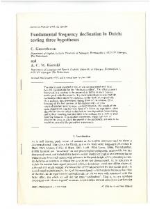
value, and these two frequency components are added together. Finally, the speech is reconstructed from the excitation and the MGC parameter stream using an MGLSA (Mel-Generalized Log Spectrum Approximation) filter [25]. The models trained by this vocoder are referred to as F0cont. C. Training of hidden Markov models We wanted to compare the modeling capacity of HMM and DNN statistical methods for the task of both traditional and continuous F0 prediction. For training the F0 contours with HMMs, the standard HTS toolkit is used [22]. In case of F0std, multi space distribution training is applied [14], whereas for F0cont, we use simple HMMs. The first and second derivatives of the parameters are also stored in the parameter files and used in the training and generation phases. Decision tree-based context clustering is used with context dependent labeling applied in the Hungarian version of HTS 2.3beta [22], [26]. Independent decision trees are built for all the parameters and duration using a maximum likelihood criterion. Although durations and MGC were also trained in the system, in the evaluation part of this paper only the modeled F0 stream is used combined with other parameters obtained from the natural sentences. D. Training of deep neural networks In this research we focused on feedforward deep neural networks. The output and input features are introduced in Table I and II and the general architecture of the network is shown on Figure 1. In the training we used the squared error loss function over minibatches. For optimization we chose ADADELTA [27] because its robustness (adaptive learning rate control, can handle noisy gradients and different data representations). To be able to discard the computational overhead of pretraining, we used rectified linear units [28] (ReLU) as activation function in the hidden layers. After preliminary experiments we changed them to parametric rectified linear units [29] (PReLU). PReLUs only slightly increase the complexity and are able to achieve better error rates by adaptively learning the shapes of activation functions. In the output layer sigmoid was used as activation function. Xavier’s weight initialization technique was used in the case of input-hidden and hiddenoutput weights [30]. We used orthogonal initialization between the hidden layers with zero bias. In the training dropout with 50% probability was applied after each layer except the output. Early stopping was applied - if the validation error did not decrease in 50 epochs, the training had been stopped. Both input and output features were transformed. The input features were standardized to have zero mean and unit variance. The output features were normalized between 0.01 and 0.99 [31]. The training samples were randomly shuffled. TABLE I. System F0std F0cont
1 2
https://github.com/idiap/ssp http://tcts.fpms.ac.be/~drugman/files/MVF.zip
OUTPUTS OF THE NEURAL NETWORK FOR F0STD AND F0CONT VOCODERS. Feature name
#
Type
LogF0
1
Continuous (interpolated)
V/UV flag
1
Binary
LogF0
1
Continuous
MVF
1
Continuous
TABLE II.
INPUTS OF THE NEURAL NETWORK.
Feature name
TABLE III.
THE WINNING 5-5 DEEP NEURAL NETWORK ARCHITECTURES OF HYPERPARAMETER OPTIMIZATION WITH MANUAL GRID SEARCH.
#
Type
Quinphone
5*68
One-hot
Number of phonemes/syllables/words/phrases in the previous/current/next syllable/word/phrase/sentence
4*3 Numerical
Number of syllables/words in the current sentence
2
Forward/backward position of the actual phoneme/syllable/ word/phrase in the syllable/word/phrase/sentence
Numerical
2*3 Numerical
(A) BASELINE (MINIBATCH SIZE=128) ID
# Hidden Layers
# Neurons
Epochs
Validation MSE
F0std-1
3
350
61
0.01076
F0std -2
3
650
32
0.01078
Phone boundaries
2
Numerical
F0std -3
3
900
30
0.01089
Percentual position of the actual frame within the phone
1
Numerical
F0std -4
3
950
36
0.01099
F0std -5
3
800
37
0.01103
Altogether:
363
(B) CONTINUOUS F0 (MINIBATCH SIZE=8) ID
X3
X363
no. of neurons
X2
no. of neurons
X1 Y1 Y2
no. of hidden layers
Figure 1. General architecture of the applied deep neural network. The Y1 and Y2 outputs are F0 and V/UV flag or F0 and MVF, in case of baseline and continuous F0, respectively.
III.
EVALUATION
In the evaluation part DNNs trained with the baseline and with the continuous F0 model took place. For training, one male and one female speaker was selected from the Precisely Labelled Hungarian Database (PLHD) containing 1984 sentences [32]. Precise labelling covers manually corrected phonetic transcription and phone boundaries. Only declarative sentences were investigated. With the male speaker, an objective evaluation was carried out first to optimize hyperparameters. Based on this objective evaluation, the top five systems were trained with the female speaker’s corpus as well. The training, validation and test data were the 80, 15 and 5 percentage of the corpus, respectively. The male and the female speakers were trained separately. In the evaluation part phone durations from natural utterances were used for the temporal information of the input vector. The deep neural network introduced in Section II.D was implemented in Torch7 deep learning framework [33], and the calculations were done on high performance NVidia GPUs. A. Objective evaluation We performed hyperparameter optimization with manual grid search. The hyperparameters introduced in Section II.D throughout remained the same and the following hyperparameters were investigated: number of hidden layers, number of neurons in hidden layers and size of the minibatches. Altogether 64 trainings were done for the baseline (F0std) system and 73 for F0cont.
# Hidden # Neurons Layers
Epochs
Validation MSE
F0cont-1
3
160
2
0.00239
F0cont-2
3
80
67
0.00346
F0cont-3
1
128
2
0.00349
F0cont-4
3
70
12
0.00352
F0cont-5
2
100
28
0.00356
In the hyperparameter optimization phase the number of hidden layers, the number of neurons and the size of the minibatch were set between 1..7, 80..2048, 8..256, respectively. The 5-5 best combinations of hyperparameters and the corresponding mean square errors on the validation set are shown in Table III. For the later analyses, we chose the F0std-1 and F0cont-1 hyperparameter sets. After the hyperparameter optimization, we measured the correlation and RMSE between the F0 curves of the natural sentences and those of obtained by the two statistical methods (HMM and DNN) combined with the two F0 modeling methods (F0std and F0cont). This calculation was done on the 5% test data for both speakers. Correlation and RMSE were only measured on the voiced frames (based on the manually labelled phonetic boundaries of the natural sentences). For calculating the correlation, we used the equation proposed by Hermes for comparing F0 contours [34]:
( , )=
∑
∑
(
(
̅)
̅ )( ∑
(
)
)
,
where x and y are two F0 contours ( ̅ and denote their means). RMSE was calculated in a standard way. The mean correlation values are shown in Figure 2. In general, the DNN statistical method resulted in lower correlation values than the HMM method for both speakers. An important result clearly visible in the figure is that F0cont has significantly higher correlation than F0std in all cases (p