Continuous Reinforcement Learning with Incremental ...

UNIVERSIDADE FEDERAL DO RIO GRANDE DO SUL INSTITUTO DE INFORMÁTICA PROGRAMA DE PÓS-GRADUAÇÃO EM COMPUTAÇÃO

RAFAEL COIMBRA PINTO

Continuous Reinforcement Learning with Incremental Gaussian Mixture Models

Thesis presented in partial fulfillment of the requirements for the degree of Doctor of Computer Science

Advisor: Prof. Dr. Paulo Martins Engel

Porto Alegre April 2017

CIP — CATALOGING-IN-PUBLICATION Pinto, Rafael Coimbra Continuous Reinforcement Learning with Incremental Gaussian Mixture Models / Rafael Coimbra Pinto. – Porto Alegre: PPGC da UFRGS, 2017. 116 f.: il. Thesis (Ph.D.) – Universidade Federal do Rio Grande do Sul. Programa de Pós-Graduação em Computação, Porto Alegre, BR– RS, 2017. Advisor: Paulo Martins Engel. 1. Reinforcement Learning. 2. Neural Networks. 3. Gaussian Mixture Models. I. Engel, Paulo Martins. II. Título.

UNIVERSIDADE FEDERAL DO RIO GRANDE DO SUL Reitor: Prof. Rui Vicente Oppermann Vice-Reitora: Profa . Jane Fraga Tutikian Pró-Reitor de Pós-Graduação: Prof. Celso Giannetti Loureiro Chaves Diretora do Instituto de Informática: Profa . Carla Maria Dal Sasso Freitas Coordenador do PPGC: Prof. João Luiz Dihl Comba Bibliotecária-chefe do Instituto de Informática: Beatriz Regina Bastos Haro

“I have no special talent. I am only passionately curious.” — A LBERT E INSTEIN

THANKS It was a long journey since my undergrad course until this point. So many things changed, including me, and yet, so many people stood by my side for all this time. One of them is my advisor, Paulo Engel, who advised me during my undergraduate thesis, my master’s thesis and now my doctoral dissertation. It’s been 8 years! I have so much to thank you, because I know I was a difficult student in so many ways, and yet you did not give up on me. Thank you very much! Also, I’m sorry for not handing you a better work as I planned... life happens (and experiments fail, too). Other person who always stood by my side, even in the darkest hours, was my girlfriend Cintia. You are the best person in the world and I’m very thankful for being with you. We’ve almost gone crazy these past few months of my research, and you did not give up on me either. Thank you very much, my love! I also thank my friends, who cheered me up when I was in most need, when even I did not believe in myself. And last but not least, I thank the ones that have been with me since I was born: my parents Rosângela and Luís Antônio, my grandmother Erotildes and my grandmother Margarida (in memoriam). I dedicate this thesis to each one of you, and also to Fabio (in memoriam), my stepfather, who, besides being a friend, did make my mother happy for 16 years. You were fantastic!

ABSTRACT This thesis’ original contribution is a novel algorithm which integrates a data-efficient function approximator with reinforcement learning in continuous state spaces. The complete research includes the development of a scalable online and incremental algorithm capable of learning from a single pass through data. This algorithm, called Fast Incremental Gaussian Mixture Network (FIGMN), was employed as a sample-efficient function approximator for the state space of continuous reinforcement learning tasks, which, combined with linear Q-learning, results in competitive performance. Then, this same function approximator was employed to model the joint state and Q-values space, all in a single FIGMN, resulting in a concise and data-efficient algorithm, i.e., a reinforcement learning algorithm that learns from very few interactions with the environment. A single episode is enough to learn the investigated tasks in most trials. Results are analysed in order to explain the properties of the obtained algorithm, and it is observed that the use of the FIGMN function approximator brings some important advantages to reinforcement learning in relation to conventional neural networks.

Keywords: Reinforcement Learning. Neural Networks. Gaussian Mixture Models.

Aprendizagem Por Reforço Contínua com Modelos de Mistura de Gaussianas Incrementais

RESUMO A contribução original desta tese é um novo algoritmo que integra um aproximador de funções com alta eficiência amostral com aprendizagem por reforço em espaços de estados contínuos. A pesquisa completa inclui o desenvolvimento de um algoritmo online e incremental capaz de aprender por meio de uma única passada sobre os dados. Este algoritmo, chamado de Fast Incremental Gaussian Mixture Network (FIGMN) foi empregado como um aproximador de funções eficiente para o espaço de estados de tarefas contínuas de aprendizagem por reforço, que, combinado com Q-learning linear, resulta em performance competitiva. Então, este mesmo aproximador de funções foi empregado para modelar o espaço conjunto de estados e valores Q, todos em uma única FIGMN, resultando em um algoritmo conciso e com alta eficiência amostral, i.e., um algoritmo de aprendizagem por reforço capaz de aprender por meio de pouquíssimas interações com o ambiente. Um único episódio é suficiente para aprender as tarefas investigadas na maioria dos experimentos. Os resultados são analisados a fim de explicar as propriedades do algoritmo obtido, e é observado que o uso da FIGMN como aproximador de funções oferece algumas importantes vantagens para aprendizagem por reforço em relação a redes neurais convencionais. Palavras-chave: Aprendizagem por Reforço, Redes Neurais, Modelos de Mistura de Gaussianas.

LIST OF ABBREVIATIONS AND ACRONYMS AING

Adaptive Incremental Neural Gas

ALE

Arcade Learning Environment

ANN

Artificial Neural Network

FIGMN

Fast Incremental Gaussian Mixture Network

GMM

Gaussian Mixture Model

GNG

Growing Neural Gas

HQSOM Hierarchical Quilted Self-Organizing Map HTM

Hierarchical Temporal Memory

I2GNG

Improved Incremental Growing Neural Gas

IGMM

Incremental Gaussian Mixture Model

IGMN

Incremental Gaussian Mixture Network

IGNG

Incremental Growing Neural Gas

ITM

Instantaneous Topological Map

MDP

Markov Decision Process

MLP

Multi-Layer Perceptron

MPF

Memory-Prediction Framework

PS

Prioritized-Sweeping

RL

Reinforcement Learning

SARSA

State-Action-Reward-State-Action

SOM

Self-Organizing Map

UCB

Upper Confidence Bound

i.i.d.

Independent and Identically Distributed

LIST OF SYMBOLS α

Learning rate for most reinforcement learning algorithms and also for a modification of the FIGMN algorithm

δ

Initial size factor for new Gaussian components in the IGMM / IGMN / FIGMN algorithms

k

Number of clusters / components

τ

Gaussian component creation threshold for IGMM / IGMN / FIGMN

ω

IGMN’s internal learning rate

LIST OF FIGURES

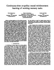
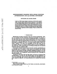
Figure 2.1 An example of multilayer perceptron architecture with 3 inputs, 2 hidden layers with 5 and 4 neurons respectively and 2 output neurons.......................20 Figure 2.2 Example of Deep Neural Network with 3 hidden layers...............................22 Figure 2.3 SOM in an advanced training state, with bidimensional inputs taken from a uniform distribution. Each node represents a data cluster, and the edges represent the neighborhood relations between them.....................................22 Figure 2.4 Example of ART architecture with 8 inputs and 6 neurons created ondemand during execution. .......................................................................................24 Figure 2.5 Example of ARTMAP architecture with 8 inputs and 6 neurons for each ART. ........................................................................................................................25 Figure 2.6 GNG in an advanced training stage with two-dimensional inputs from a uniform distribution. ...............................................................................................25 Figure 2.7 Example of a two-dimensional ITM with 66 clusters constructed from a single pass through data. ......................................................................................28 Figure 2.8 An example of IGMN with 3 input nodes and 5 Gaussian components. Any input element can be predicted by using any other element, which means that the input vector can actually be divided into input and output elements.........29 Figure 2.9 An example of IGMN with 3 input nodes and 5 Gaussian components. Two of the input elements were selected for estimating the third one. The different color intensities inside each Gaussian component represent their different posterior probabilities after seeing data xi (only the given elements), and are used to weight the contributions of each component to the final result. ...........32 Figure 4.1 A tile coding structure with 2 4x3 tilings. The given point activates 1 cell in each tiling.....................................................................................................46 Figure 4.2 An RBF gaussian receptive field. Activation increases as the point gets near to the receptive field center. ............................................................................47 Figure 4.3 Some examples of bidimensional Fourier basis functions. ...........................50 Figure 4.4 A topographic map generated by the neural fields approach with 3 activity blobs. .............................................................................................................52 Figure 4.5 Example of a learned ITPM model with 2 units mapping to different regions of a robot trajectory. ...................................................................................54 Figure 4.6 The ADHDP architecture. The J is used in the control literature instead of the Q value..........................................................................................................56 Figure 4.7 Wirefitting with 3 wires before and after update according to selected action (red dot). Each point contains the action itself and its Q value. ..................56 Figure 4.8 Step-by-step representation of the CMAES algorithm. CEM and PI2 produce similar behavior, except that PI2 does not change the size or shape of the Gaussian. ...........................................................................................................59 Figure 5.1 Training and testing times for both versions of the IGMN algorithm with growing number of dimensions ......................................................................74 Figure 5.2 FIGMN-Q: The FIGMN models the densities of the input space and feeds likelihoods to linear Q-learning. Resulting states, rewards and actions are used in the learning algorithm...........................................................................75 Figure 5.3 Unified FIGMN-Q: The FIGMN models the densities of the joint space of states and Q-values. Resulting states, rewards and actions are used in the learning algorithm, which is embedded into the FIGMN itself. .............................76

Figure 5.4 In this case, the FIGMN models the densities of the joint space of states, actions and Q-values. Resulting states and rewards are used in the learning algorithm, which is embedded into the FIGMN itself. ...........................................76 Figure 5.5 The mountain car environment running inside OpenAI Gym. ......................78 Figure 5.6 The cart-pole environment running inside OpenAI Gym..............................79 Figure 5.7 The acrobot environment running inside OpenAI Gym. ...............................80 Figure 5.8 Example of a single evaluation of the FIGMN-Q algorithm on the mountain car v0 environment...........................................................................................80 Figure 5.9 Example of a single evaluation of the FIGMN-Q algorithm on the cartpole v0 environment................................................................................................81 Figure 5.10 Example of a single evaluation of the FIGMN-Q algorithm on the acrobot v0 environment. .............................................................................................81 Figure 5.11 Example of a single evaluation of the Unified FIGMN-Q algorithm on the cart-pole v0 environment. .................................................................................81 Figure 5.12 Example of a single evaluation of the Unified FIGMN-Q algorithm on the cart-pole v1 environment. .................................................................................82 Figure 5.13 Example of a single evaluation of the Unified FIGMN-Q algorithm on the acrobot v1 environment.....................................................................................82 Figure 5.14 Example of a single evaluation of the Unified FIGMN-Q algorithm on the mountain car v0 environment............................................................................82 Figure 5.15 Policy learned by the U-FIGMN-Q algorithm on the mountain car task. The coloured bands are just very elongated ellipses...............................................84 Figure 6.1 Visualizing the proposed component creation criterion modification. Left: the model is composed by 2 Gaussian components and new data (the cross) arrives. Middle: How the current component creation criterion would behave. The closest component is not good enough, so a new component is created, resulting in overfitting. Right: How the proposed component creation criterion would behave. The model is sufficiently complex to model the new point withouth creating new components. .......................................................................88 Figure 6.2 Visualizing the proposed component initial size adaptation. Left: the model is composed by 1 Gaussian component and new data (the cross) arrives. Middle: How the current component initial size would behave, considering large enough δ. It overlaps the existing component, resulting in catastrophic forgetting in its topmost region. Right: How the proposed component adaptive initialization would behave. The initial size is reduced to avoid overlap. .......88

LIST OF TABLES

Table 5.1 Table 5.2 Table 5.3 Table 5.4 Table 5.5

Datasets ...........................................................................................................71 Accuracy of different algorithms on standard datasets ...................................72 Number of Gaussian components created .......................................................72 Training and testing running times (in seconds) .............................................72 Number of episodes to solve each task. ..........................................................78

CONTENTS 1 INTRODUCTION.......................................................................................................14 1.1 Motivation................................................................................................................14 1.2 Research Overview .................................................................................................15 1.3 Methodology ............................................................................................................16 1.4 Contributions...........................................................................................................17 1.5 Publications .............................................................................................................18 1.6 Work Structure .......................................................................................................19 2 BASE LEARNING ALGORITHMS.........................................................................20 2.1 Multi-Layer Perceptron..........................................................................................20 2.1.1 Deep Neural Networks...........................................................................................21 2.2 Self-Organizing Map (SOM)..................................................................................22 2.3 Adaptive Resonance Theory (ART) ......................................................................23 2.4 Growing Neural Gas (GNG) ..................................................................................25 2.5 Incremental GNG (IGNG) .....................................................................................27 2.6 Incremental Gaussian Mixture Network ..............................................................28 2.6.1 Learning .................................................................................................................29 2.6.2 Creating New Components ....................................................................................31 2.6.3 Removing Spurious Components ..........................................................................32 2.6.4 Inference ................................................................................................................32 2.7 Conclusion ...............................................................................................................33 3 REINFORCEMENT LEARNING ............................................................................34 3.1 TD-Learning............................................................................................................35 3.2 SARSA .....................................................................................................................36 3.2.1 Exploration-Exploitation Dilemma........................................................................37 3.3 Q-Learning ..............................................................................................................37 3.4 Dyna-Q .....................................................................................................................38 3.5 R-Max.......................................................................................................................38 3.6 Delayed Q-Learning................................................................................................39 3.7 RTMBA....................................................................................................................40 3.8 Conclusion ...............................................................................................................40 4 CONTINUOUS REINFORCEMENT LEARNING................................................42 4.1 Continuous States ...................................................................................................44 4.1.1 Linear Function Approximation ............................................................................44 4.1.2 Tile Coding ............................................................................................................45 4.1.3 Radial Basis Function Neural Network .................................................................46 4.1.4 Multi-Layer Perceptron..........................................................................................47 4.1.5 Instantaneous Topological Map (ITM) ..................................................................48 4.1.6 Fourier Basis Functions .........................................................................................49 4.2 Continuous Actions.................................................................................................50 4.2.1 Sequential Monte Carlo .........................................................................................50 4.2.2 Self-Organizing Map (SOM) .................................................................................51 4.2.3 Adaptive Resonance Theory ..................................................................................52 4.2.4 Neural Fields..........................................................................................................52 4.2.5 Hedger....................................................................................................................53 4.2.6 ITPM ......................................................................................................................54 4.2.7 CACLA ..................................................................................................................55 4.2.8 ADHDP..................................................................................................................55 4.2.9 Wire-fitted Neural Network Q-Learning................................................................56

4.2.10 Growing Neural Gas (GNG) ................................................................................57 4.2.11 Gaussian Mixture Model Reinforcement Learning .............................................57 4.2.12 IGMN...................................................................................................................58 4.2.13 Policy Search Methods ........................................................................................58 4.3 Continuous Time.....................................................................................................60 4.3.1 Q-Learning for SMDPs..........................................................................................61 4.3.2 Advantage Updating ..............................................................................................62 4.3.3 Continuous Actor Critic.........................................................................................63 4.4 Conclusions..............................................................................................................64 5 PROPOSED ALGORITHMS....................................................................................65 5.1 Fast IGMN ...............................................................................................................66 5.1.1 Experiments and Results........................................................................................71 5.2 Reinforcement Learning with FIGMN .................................................................74 5.2.1 Experiments and Results........................................................................................75 5.3 Conclusions..............................................................................................................85 6 DISCUSSION AND FUTURE WORKS...................................................................86 REFERENCES...............................................................................................................90 APPENDIX A — RESUMO EM PORTUGUÊS ......................................................101 A.1 Introdução.............................................................................................................101 A.1.1 Motivação............................................................................................................102 A.1.2 Visão Geral da Pesquisa......................................................................................102 A.1.3 Metodologia ........................................................................................................103 A.1.4 Contribuições ......................................................................................................104 A.2 Algoritmos Propostos...........................................................................................105 A.3 Fast IGMN ............................................................................................................106 A.3.1 Experimentos e Resultados .................................................................................107 A.4 Aprendizagem por Reforço com a FIGMN .......................................................109 A.4.1 Experimentos e Resultados .................................................................................110 A.5 Conclusões.............................................................................................................114

14

1 INTRODUCTION

Reinforcement learning has become mainstream in the last few years, mainly due to the efforts of the Google Deep Mind team. They have managed both to achieve humanlevel gameplay on Atari games [Mnih et al. 2015] and to defeat the go world champion [Silver et al. 2016], and reinforcement learning is at the heart of both achievements, through an algorithm called Deep Q-Learning Network (DQN). That’s not just a matter of preference or hype, but an acknowledgment of the virtues of reinforcement learning for producing intelligent agents with high-quality autonomous behaviors with minimal human supervision. It is an excellent paradigm for allowing learning from sparse rewards without explicit goals or continuous human supervision, just like living beings. This makes reinforcement learning an obvious candidate for advancing the fields of artificial intelligence and autonomous robots. Yet, albeit being the state-of-the-art on those tasks, the mentioned approaches suffer from low data efficiency, which means that a high number of training episodes is necessary for the agent to acquire the desired level of competence on diverse tasks. Deep Mind’s algorithms require millions of agent-environment interactions due to very inefficient learning. This is not acceptable for some classes of tasks, such as robotics, where failure and damage must be minimized. There are solutions for this problem, but most of them deal with discrete environments instead of continuous environments, i.e., environments with an infinite number of states and possibly infinite actions too, like the physical world, as will be shown in chapter 3. [Gu et al. 2016] presented a solution for augmenting DQN with model-based learning, but the results are still far from ideal, possibly due to its reliance on non-data-efficient function approximators like neural networks (they require many epochs in order to approximate their target functions, at least with the most commonly used optimization procedures). This research proposes a new solution to this problem, by integrating a sample-efficient function approximator with reinforcement learning techniques, reducing the number of required interactions with the real environment.

1.1 Motivation

Current approaches for solving reinforcement learning tasks in continuous domains often employ neural networks as function approximators. This has proven to be an effective approach for solving hard reinforcement learning tasks. However, slowly and

15

iteratively approximating the Q-value function is often the case, which is not acceptable for robotics and real-world tasks in general. A robot cannot afford to fall from stairs one thousand times before learning to avoid them. More data-efficient algorithms are necessary. In the ideal case, a single episode should be enough to learn a given task. While other works focus on the reinforcement learning side itself for data efficiency, the function approximation side is often neglected. Hence, this is the focus of this research: integrate data-efficient function approximators with reinforcement learning in order to offer a complementary solution to other acceleration methods.

1.2 Research Overview

The proposed solution to the mentioned issues in the previous section consists in developing a reinforcement learning algorithm based on the Incremental Gaussian Mixture Network (IGMN) [Heinen and Engel 2011]. The IGMN is capable of learning useful models in a single-pass through data, which greatly reduces the amount of interaction necessary for learning in a physical environment, where data is costly. It also provides variance estimates for its predictions, which can be used to guide exploration of promising actions and to avoid excessive exploration of hopeless actions [Heinen, Bazzan and Engel 2011]. Finally, it is able to infer any of its variables from any other set of variables. It means that it could be used to predict expected rewards, select actions and predict consequences of its actions (a forward model) all in a single model, if wanted. A modelfree (without a forward model) approach for combining the IGMN with reinforcement learning was presented in [Heinen 2011], but it was not the focus of the research and data efficiency was not analysed. The feasibility and properties of this idea are going to be explored in this research. A less synergistic approach where the IGMN only models the state-space density is going to be explored first, and then, using the same IGMN to model the state space and to approximate a Q-value function will be the next step. Both approaches are presented in chapter 5. But the IGMN has its drawbacks too: it has cubic complexity on the number of dimensions of data. If we want to provide a solution for real-world tasks (most of which are high dimensional), it is not acceptable. Thus, before applying it to reinforcement learning, reducing the time complexity of the IGMN algorithm is mandatory. The process for achieving this goal and the resulting algorithm update will also be shown in chapter 5. In order to explore these ideas, the following research questions were selected:

16

• Can the complexity of the IGMN algorithm be reduced by avoiding matrix inversions? • In which forms can the IGMN algorithm be used as a function approximator for reinforcement learning? • How can it be used to approximate the state space only? • How can it learn the joint distribution of states and Q-values in a single model? • Does the resulting algorithm increase the data-efficiency of reinforcement learning?

1.3 Methodology

Regarding the need to answer the first research question, about reducing the IGMN complexity, experiments were conducted in the Weka [Hall et al. 2009] platform using the Java programming language. This platform allows for measuring and comparing the running time of various algorithms in various datasets (which are distributed along with Weka). If complexity is indeed reduced, reductions in runtime compared to the original IGMN are expected, and these reductions should be more drastic as the number of dimensions of the datasets increases (the complexity reduction is related to the number of dimensions). Also, the resulting algorithm must give exactly the same results as the original one. In order to answer the remaining questions, testing and comparing reinforcement learning algorithms is necessary. Three items are required for this: • Proposed algorithms; • Environments / tasks; • Competing algorithms. Besides taking a long time to implement and the risk of reinventing the wheel, the last two items would remove focus from the important part of this work, which are the proposed algorithms. The best solution found to solve this problem is to use the OpenAI Gym [Brockman et al. 2016] as the primary platform for testing the proposed algorithms. This recently released open-source platform provides dozens of ready-to-use reinforcement learning environments as well as a leaderboard-like page comparing the performance of algorithms from different users, including the most common algorithms like Q-learning. The performance is measured by two factors: episodes to solve (data efficiency) and

17

mean reward. Each environment has some accumulated reward to reach. More precisely, the agent must obtain an average accumulated reward equal or higher than the goal for 100 consecutive episodes. Time to solve is defined as the first episode of the successful 100 episode window. Authors should publish, together with their algorithms, precise instructions for reproductions. This greatly improves the scientific value of this approach. Considering that the research questions refer to possibilities and capabilities, rather than to performance, only sufficiently competitive results will be expected. If an algorithm solves a task, it is considered that "it works". Anyway, each algorithm will be tested on various environments to be sure of their generality. With that said, more demanding tasks like the Atari games [Bellemare et al. 2013] will be avoided, due to hardware restrictions. All experiments are being executed on an Intel i7 laptop without access to GPU. Using compute services or even the university cluster platform would not give large improvements, since the IGMN algorithm is not trivially parallelized due to its incremental nature. Since the OpenAI Gym platform currently only supports the Python language, this was the language of choice for implementing the final experiments. An existing open-source implementation 1 of the IGMN algorithm in this language was used at first. This implementation was already used with success in previous works [Pereira, Engel and Pinto 2012]. Later, it was converted into the more scalable FIGMN algorithm which is part of the contributions of this research.

1.4 Contributions

This research contributes to the field of machine learning through the Fast IGMN algorithm presented in chapter 5. It comprises an online EM procedure devoid of matrix inversions and full determinant computations. It also presents formulations for Gaussian mixture regression using the inverse covariance matrix directly. This is an important piece for the remaining algorithms to be implemented. Continuous-time reinforcement learning in continuous state spaces through the use of an FIGMN function approximator is presented too as a novel contribution. Moreover, the main contribution of this work consists in a algorithm combining the FIGMN with Q-Learning for reinforcement learning with continuous states, learning in the joint state and Q-values space. With this, a more data-efficient reinforcement learning algorithm 1

https://github.com/renatopp/liac/blob/master/liac/models/igmn.py

18

is expected as the final result, which should be more appropriate for robotics tasks and also fills most of the requirements mentioned in chapter 4. The proposed architecture will be tested on classic reinforcement learning problems provided by the OpenAI Gym [Brockman et al. 2016] platform. Finally, an extensive and up-to-date survey of the reinforcement learning field is provided. The most cited survey on the field [Kaelbling, Littman and Moore 1996] dates from 1996, while most recent ones deal with restricted types of reinforcement learning only, like multi-agent systems, robotics or transfer learning.

1.5 Publications

The following papers which have me as the first author were published during my Ph.D. research: • One-Shot Learning in the Road-Sign Problem [Pinto, Engel and Heinen 2012]: International Joint Conference on Neural Networks (IJCNN 2012), Qualis A2. • A Fast Incremental Gaussian Mixture Model [Pinto and Engel 2015]: Plos One, Qualis B2 (A1 until acceptance date). Submitted: • Scalable and Incremental Learning of Gaussian Mixture Models (2017): Annals of Mathematics and Artificial Intelligence, Qualis B1. Other published papers where I contributed as a co-author: • Using a Gaussian Mixture Neural Network for Incremental Learning and Robotics [Heinen, Engel and Pinto 2012]: International Joint Conference on Neural Networks (IJCNN 2012), Qualis A2. • Autocorrelation and partial autocorrelation functions to improve neural networks models on univariate time series forecasting [Flores, Engel and Pinto 2012]: International Joint Conference on Neural Networks (IJCNN 2012), Qualis A2. • Learning Abstract Behaviors with the Hierarchical Incremental Gaussian Mixture Network [Pereira, Engel and Pinto 2012]: Brazilian Symposium on Neural Networks (SBRN 2012), Qualis B3.

19

1.6 Work Structure

Chapters 2 to 4 present bibliographical research and related works in different areas: Chapter 2 presents static learning algorithms, which serve as the basis for function approximation in reinforcement learning; Chapter 3 deals with general reinforcement learning algorithms while chapter 4 deals with continuous reinforcement learning algorithms. Finally, chapter 5 presents the contributions of this research, including experimental results, and chapter 6 finishes this work with discussions and future works.

20

2 BASE LEARNING ALGORITHMS

This chapter presents a review of supervised and unsupervised learning algorithms. These algorithms will serve as function approximators for continuous state reinforcement learning algorithms to be presented in chapter 4.

2.1 Multi-Layer Perceptron

The multilayer perceptron (MLP) is a supervised feedforward artificial neural network model that learns non-linear mappings from input vectors to output vectors (discrete or continuous). It is composed of multiple layers of non-linear neurons (computational units) which propagate signals until they reach the output layer. Each neuron computes the scalar product between its inputs and its incoming weights and then applies some nonlinear transformation, usually a sigmoid function. Consecutive layers are fully connected and the number of neurons in each of them (as well as the number of layers) must be manually specified. This architecture can be seen in figure 2.1. Once the signal reaches the output layer, the error of the computed values in relation to the given output example (the target values) is back-propagated in order to update the network weights. This training procedure can be performed in various ways, but here we will talk about the Stochastic Gradient Descent (SGD) procedure, since it can be used for online learning, i.e. updating the model after each example data is presented to the network. The specialized version of SGD for multilayer perceptrons is called Stochastic Backpropagation [Werbos 1974]. Backpropagation tries to minimize a cost function, usually the mean squared error, in relation to the network weights between the neurons. Unlike single layer neural networks (e.g. perceptron, adaline), there is no guarantee of

Figure 2.1 – An example of multilayer perceptron architecture with 3 inputs, 2 hidden layers with 5 and 4 neurons respectively and 2 output neurons.

21

finding the global minimum, just local minima, since the error surface is not convex. Also, this kind of training procedure requires many epochs for convergence, i.e. scanning the entire dataset many times for reducing error at small steps. It is also proven that multilayer perceptrons are universal function approximators [Maxwell and White 1989], given the necessary number of neurons. Nevertheless, it is not guaranteed that backpropagation can find those approximations even with enough neurons. In contrast to Radial Basis Function (RBF) networks, which use local activation functions (a more complete description can be found in section 4.1.3), the MLP is a global algorithm, meaning that all of its neurons contribute to its output at any region of inputspace. An undesirable consequence of this is catastrophic forgetting, when new information overwrites old information in the network weights. Some techniques are necessary to mitigate this problem when applying an MLP to reinforcement learning, such as the use of experience replay (storing experiences for reuse) [Lin 1992].

2.1.1 Deep Neural Networks

Deep learning [Arel, Rose and Karnowski 2010, Schmidhuber 2015, Bengio and Courville 2016] refers to algorithms capable of autonomously extracting features and create deeper abstractions over them. More specifically, deep neural networks (see figure 2.2) are the deep learning version of multi-layer perceptrons, with diverse adjustments for working with many layers, like unsupervised pre-training [Bengio et al. 2007], ReLU activation functions [Glorot, Bordes and Bengio 2011], dropout regularization [Hinton et al. 2012] and batch normalization [Ioffe and Szegedy 2015]. Deep neural networks are achieving state-of-the-art performance on classification tasks for various datasets such as MNIST [Wan et al. 2013], CIFAR-10 [Graham 2014], CIFAR-100 [Clevert, Unterthiner and Hochreiter 2015], STL-10 [Zhao et al. 2015], SVHN [Lee, Gallagher and Tu 2016] and ImageNet [Russakovsky et al. 2015]. However, large clusters of CPU’s and GPU’s are needed in order to run these models in moderate time. Also, when dealing with reinforcement learning, proper modifications, such as experience replay, are necessary in order to mitigate the inherent problems of the multilayer perceptron.

22

Figure 2.2 – Example of Deep Neural Network with 3 hidden layers. 2.2 Self-Organizing Map (SOM)

Figure 2.3 – SOM in an advanced training state, with bidimensional inputs taken from a uniform distribution. Each node represents a data cluster, and the edges represent the neighborhood relations between them. The SOM is an unsupervised neural network, meaning it does not learn from inputoutput example pairs, instead just learning the structure of the input space, in this case in the form of data clusters. It consists of a single competitive layer (besides the input layer) neural network, and this layer is spatially organized. It’s usually a 2D lattice (could be 1D, 3D or any dimension) and, therefore, the relative position of the neurons is important, in contrast to more conventional neural networks (a 2D input space representation in this architecture can be seen in figure 2.3). The weights from the input layer to the competitive layer represent the learned input vectors’ prototypes and, therefore, have the same dimensionality as the input space. The input vectors are presented one-by-one to the algorithm, which finds the most similar prototype so far, based on a distance metric (usually Euclidian or Manhattan distance). The best matching neuron is then selected as

23

the winner neuron or best matching unit (BMU), according to the following equation: b(t) = arg min{kx(t) − wi k} , i∈VO

(2.1)

where x(t) is the input vector at time t, b(t) is the index (position) of the winner neuron at time t in the output / competitive layer space VO , wi (t) is a prototype to be compared to the input, also at time t. After finding the winner neuron, its corresponding weights wb (its prototype vector elements) are adjusted, as well as the weights of its neighbors, according to the following update rule: wi (t + 1) = wi (t) + γ(t)hib (t)(x(t) − wi (t)) ,

(2.2)

where γ is a learning rate between 0 and 1 and hib is a neighborhood function such as  hib (t) = exp

−kIi − Ib k2 2σ(t)2

 ,

(2.3)

where Ii and Ib are neurons i and b indexes (positions) on the competitive layer, and σ(t) is the Gaussian standard deviation at time t. Note that γ and σ are time dependent, and are usually implemented with some decay during the algorithm’s execution time.

2.3 Adaptive Resonance Theory (ART)

Adaptive Resonance Theory (ART) [Carpenter and Grossberg 1986] differs from other works by its foundation on neuroscience and its dual characteristic: it is both a cognitive theory and a set of biologically plausible computational models, the later being the focus of interest here. The first ART model (also called ART1) deals with boolean variables only. Its innovative feature lies in the fact that new neurons are created when existing ones are not enough to recognize (or to "resonate" with) incoming inputs. This mechanism is controlled by a vigilance meta parameter. Although the complete model is complex, including differential equations and continuous time, [Moore 1989] described it very simply by using the clustering paradigm: Whenever the input is well reconstructed, i.e., its similarity to the best matching unit is larger than the vigilance parameter, the best matching unit is updated to be closer to the input. However, if this condition is not met, a new neuron is created to recognize the input perfectly (its weights are initialized equal to the input).

24

Another interesting feature which is relevant to the present work is that it is suggested that this vigilance parameter may be automatically modulated by reinforcement from the environment [Carpenter and Grossberg 1987]. If an incorrect recognition is followed by negative reinforcement, the vigilance parameter is increased as a form of greater attention on some poorly understood part of the environment. This is in conformity with this research’s goal of achieving synergy between algorithms. See figure 2.4 for a depiction of the ART architecture.

Figure 2.4 – Example of ART architecture with 8 inputs and 6 neurons created on-demand during execution.

The ART2 [Carpenter and Grossberg 1987] improves upon the ART1 model by dealing with real-valued inputs, while ART2-A [CARPENTER, GROSSBERG and ROSEN 1991] improves its speed. FuzzyART [Carpenter, Grossberg and Rosen 1991] extends ART with fuzzy min and max operators, replacing the and and or operators, respectively. It also introduces complement coding, a normalization procedure where the absence of features is explicitly represented, keeping the norm of inputs constant. ARTMAP [Carpenter, Grossberg and Reynolds 1991] employs 2 ART models, one for inputs and other for outputs, allowing it to perform supervised learning. The output ART is also capable of modulating the vigilance parameter of the input ART in order to minimize prediction errors (see figure 2.5 for an example). Finally, a Fuzzy ARTMAP was proposed in [Carpenter et al. 1992], which adds fuzzy operators to ARTMAP.

25

Figure 2.5 – Example of ARTMAP architecture with 8 inputs and 6 neurons for each ART.

Figure 2.6 – GNG in an advanced training stage with two-dimensional inputs from a uniform distribution.

2.4 Growing Neural Gas (GNG)

An improvement over the Neural Gas algorithm [Martinetz and Schulten 1991], the Growing Neural Gas (GNG) is an unsupervised neural network similar to the SOM, but capable of learning the topology and the number of necessary neurons for a given task. Here is a description of the algorithm: 1. Start with 2 neurons a and b at random positions wa and wb from the input space Rn . 2. Read an input vector v. 3. Find the neuron s1 nearest to the input vector v and the second nearest neuron, s2 .

26

4. Increment the age of all connections of s1 . 5. Add the square distance between the input vector and the winning neuron s1 in the input space to an error accumulator for this neuron: ∆error(s1 ) = kws1 − vk2 .

(2.4)

6. Move s1 and its neighbors towards v by fractions b and n (learning rates), respectively, of the total distance: ∆ws1 = b (v − ws1 ) ,

(2.5)

∆wn = n (v − wn ) .

(2.6)

7. If s1 and s2 are connected, reset this connection’s age to 0. Otherwise, connect both neurons. 8. Remove connections older than amax . If this results in neurons without connections, remove those neurons too. 9. If the number of input vector presented so far is a multiple of a λ parameter, insert a new neuron the following way: • Find the neuron q with the largest accumulated error. • Insert a new neuron r midway between q and its neighbor f with the largest accumulated error: wr = 0.5(wq + wf ) .

(2.7)

• Connect the new neuron r with neurons q and f, and remove the original connection between q and f. • Decrease the error accumulators of q and f by multiplying them by a constant α. Initialize the error accumulator of r with the new error accumulator value of q. 10. Decrease all error accumulators by multiplying them by a constant d. 11. If a stopping criterion (e.g., network size or performance measure) is still not met, go to step 2. An example of a GNG in advanced training state can be seen in figure 2.6.

27

2.5 Incremental GNG (IGNG)

A variation of the GNG, called Incremental GNG (IGNG), is proposed in [Prudent and Ennaji 2005], with an important difference: its growing mechanism does not depend on time, but on instantaneous errors. The IGNG is more appropriate for lifelong tasks, since it will not add neurons indefinitely. This new mechanism works in a form similar to ART’s vigilance parameter. If the current input ξ is too distant (as defined by a meta parameter σ) from its best matching unit, a new "embryo" neuron is created with its center at ξ. If the current input is sufficiently close to its best matching unit but not from the second nearest neuron, a new neuron is created the same way as before, but now a connection between it and the BMU is also added. If the current input is sufficiently close both its nearest and second nearest neurons, the BMU and its neighbors are updated as vanilla GNG. Neurons have a "maturation time" defined by the meta parameter amax . Only mature neurons can be removed when they have no edges. These improvements are essential for tasks like the ones studied in this work, since robotics might deal with unlimited data streams. An improved version of the IGNG called Improved Incremental Growing Neural Gas (I2GNG) is presented in [Hamza et al. 2008], with the additional property of setting different distance thresholds for each neuron, according to the spread of its data. Another approach for computing different thresholds for each neuron is presented in [Shen and Hasegawa 2010] with the Self-Organizing Incremental Neural Network (SOINN), where the threshold is defined by the neuron’s distance to its nearest neighbor. More recently, the work presented in [Bouguelia, Belaïd and Belaïd 2013] shows a new algorithm called Adaptive Incremental Neural Gas (AING), which is similar to IGNG and its variants, with an additional goal: to be parameter-free. This feature is important when dealing with data streams and lifelong tasks in general, since we have less information about the data distribution in order to select adequate meta parameters. This goal is achieved by using a distance threshold which is a combination of I2GNG and SOINN approaches, while setting each neuron’s learning rate to

1 |xy |

(the inverse of the number of data points

associated with neuron y). Finally, Jockusch and Ritter (1999) propose another approach (which predates IGNG) for a GNG-like algorithm appropriate for data streams, the Instantaneous Topological Map (ITM). It works by constructing a Delaunay triangulation of data incrementally (see figure 2.7). This criterion alone can deal with creation and removal of neurons, leaving only one meta parameter for the ITM, which controls its den-

28

sity. Neuron updating is optional and needs a learning rate when used. It was verified in my current research that adopting an AING-like automatic learning rate improves the quality of the resulting network, decreasing the number of necessary neurons.

Figure 2.7 – Example of a two-dimensional ITM with 66 clusters constructed from a single pass through data.

2.6 Incremental Gaussian Mixture Network

The Incremental Gaussian Mixture Network (IGMN) [Heinen 2011] is a supervised algorithm that uses as its base an incremental approximation of the EM algorithm [Dempster et al. 1977]. It creates and continually adjusts a probabilistic model consistent with all sequentially presented data, after each data point presentation, and without the need to store any past data points (this is how we define "incremental" in this work). Its learning process is sample-efficient, meaning that only a single scan through the data is necessary to obtain a consistent model. Together with the ART, AING, SOINN and ITM, the IGMN is are able to learn from single data points and discard them thereafter, as opposed to batch learning, which requires the entire dataset beforehand and requires full retraining when new data points arrive. But differently from these other sample-efficient algorithms, IGMN adopts a Gaussian mixture model of distribution components that can be expanded to accommodate new information from an input data point, or reduced if spurious components are identified along the learning process. Each data point assimilated by the model contributes to the

29

sequential update of the model parameters based on the maximization of the likelihood of the data. The parameters are updated through the accumulation of relevant information extracted from each data point. Since each component is a multivariate Gaussian, in contrast to other methods which only store means, the IGMN is more expressive and has higher generalization capabilities (each component is a linear regressor itself and is not restricted to local approximations). The IGMN is capable of supervised learning, simply by assigning any of its input vector elements as outputs (any element can be used to predict any other element, like auto-associative neural networks [Rumelhart and McClelland 1986]). This architecture is depicted in figure 2.8. Next subsections describe the algorithm in more detail.

Figure 2.8 – An example of IGMN with 3 input nodes and 5 Gaussian components. Any input element can be predicted by using any other element, which means that the input vector can actually be divided into input and output elements.

2.6.1 Learning

The algorithm starts with a single component centered at the first data point, and more components are created as necessary (see subsection 2.6.2). Given input x (a single instantaneous data point), the IGMN algorithm processing step is as follows. First, the squared Mahalanobis distance d2 (x, j) for each component j is computed: d2M (x, j) = (x − µj )T Σ−1 j (x − µj ) ,

(2.8)

where µj is the j th component mean, Σj its full covariance matrix . If any d2 (x, j) is smaller than χ2D,1−β (the 1 − β percentile of a chi-squared distribution with D degrees-offreedom, where D is the input dimensionality and β is a user defined meta-parameter, e.g., 0.1), an update will occur, and posterior probabilities are calculated for each component

30

as follows:   1 1 2 p p(x|j) = exp − dM (x, j) , 2 (2π)D/2 |Σj | p(j|x) =

p(x|j)p(j) ∀j , K X p(x|k)p(k)

(2.9)

(2.10)

k=1

where K is the number of components. Now, parameters of the algorithm must be updated according to the following equations: vj (t) = vj (t − 1) + 1 ,

(2.11)

spj (t) = spj (t − 1) + p(j|x) ,

(2.12)

ej = x − µj (t − 1) ,

(2.13)

p(j|x) , spj

(2.14)

∆µj = ωj ej ,

(2.15)

µj (t) = µj (t − 1) + ∆µj ,

(2.16)

e∗j = x − µj (t) ,

(2.17)

T Σj (t) = (1 − ωj )Σj (t − 1) + ωj e∗j e∗T j − ∆µj ∆µj ,

(2.18)

ωj =

p(j) =

spj , M X spq

(2.19)

q=1

where spj and vj are the accumulator and the age of component j, respectively, and p(j) is its prior probability. The equations are derived using the Robbins-Monro stochastic approximation [Robbins and Monro 1951] for maximizing the likelihood of the model.

31

This derivation can be found in [Engel and Heinen 2011, Engel 2009].

2.6.2 Creating New Components

If instead of having any p¯(x|j) greater than a threshold τmax , we have all p¯(x|j) below some threshold τmin (e.g., 0.001) (or there are no components) and a stability criterion is satisfied, which means having all vj greater than some agemin (e.g., D + 1, where D is the input space dimensionality; this only applies to data-flows which vary slowly in time, such as most time-series and real-world signals, such as sonar data from a mobile robot, otherwise, agemin = 0 would be better), then a new component j is created and initialized as follows: µj = x;

spj = 1;

vj = 1;

p(j) =

1 K X

;

2 Σj = σini I,

spi

i=1

where K already includes the new component and σini can be obtained by: σini = δstd(x) ,

(2.20)

where δ is a manually chosen scaling factor (e.g., 0.01) and std is the standard deviation of the dataset. Note that the IGMN is an online and incremental algorithm and therefore it may be the case that we do not have the entire dataset to extract descriptive statistics. In this case the standard deviation can be just an estimation (e.g., based on sensor limits from a robotic platform), without impacting the algorithm. In recent implementations, a feature called auto − τmin was added, which adjusts the τmin parameter automatically. Its workings are straightforward: whenever a component is created, store the largest p¯(x|j) obtained in that time step (which should be smaller than τmin , according to the component creation rule). If this new component is removed later, set taumin to its stored p¯(x|j) value. The rationale is that if some component is created according to some p¯(x|j) and later this component is removed, then taumin is being too tolerant and should be reduced to avoid creating another component in the same situation again.

32

2.6.3 Removing Spurious Components

Optionally, a component j is removed whenever vj > vmin and spj < spmin , where vmin and spmin are manually chosen (e.g., 5.0 and 3.0, respectively). In that case, also, p(k) must be adjusted for all k ∈ K, k 6= j, using (2.19). In other words, each component is given some time vmin to show its importance to the model in the form of an accumulation of its posterior probabilities spj . Those components are entirely removed from the model instead of merged with other components, because we assume they represent outliers. Since the removed components have small accumulated activations, it also implies that their removal has almost no negative impact on the model quality, often producing positive impact on generalization performance due to model simplification (a more throughout analysis of parameter sensibility for the IGMN algorithm can be found in [Heinen 2011]).

2.6.4 Inference

Figure 2.9 – An example of IGMN with 3 input nodes and 5 Gaussian components. Two of the input elements were selected for estimating the third one. The different color intensities inside each Gaussian component represent their different posterior probabilities after seeing data xi (only the given elements), and are used to weight the contributions of each component to the final result.

In the IGMN, any element can be predicted by any other element. In other words, inputs and targets are presented together as inputs during training. Thus, inference is done by reconstructing data from the target elements (xt , a slice of the entire input vector x) by estimating the posterior probabilities using only the given elements (xi , also a slice of the

33

entire input vector x), as follows: p(j|xi ) =

p(xi |j)p(j) M X

∀j .

(2.21)

p(xi |q)p(q)

q=1

It is similar to (2.10), except that it uses a modified input vector xi with the target elements xt removed from calculations. After that, xt can be reconstructed using the conditional mean equation: xˆt =

M X

p(j|xi )(µj,t + Σj,ti Σ−1 j,i (xi − µj,i )) ,

(2.22)

j=1

where Σj,ti is the sub-matrix of the jth component covariance matrix associating the unknown and known parts of the data, Σj,i is the sub-matrix corresponding to the known part only and µj,i is the jth’s component mean without the element corresponding to the target element. This division can be seen below:  Σj = 

Σj,i Σj,it Σj,ti

Σj,t

 .

The inference procedure is depicted in figure 2.9. It is also possible to estimate the conditional covariance matrix for a given input, which allows us to obtain error margins for the inference procedure. It is computed according to the following equation: ˆ Σ(t) = Σj,t − Σj,ti Σ−1 j,i Σj,it .

(2.23)

2.7 Conclusion

This chapter reviewed six incremental supervised learning algorithms and their variants, namely: multi-layer perceptron, self-organizing map, adaptive resonance theory, growing neural gas, incremental neural gas and incremental Gaussian mixture network. Among those, adaptive resonance theory, incremental neural gas and incremental Gaussian mixture network are the most appropriate for the proposed work, since they can grow and shrink as necessary, rendering the resulting agent more adaptive to different environments with less meta parameter tuning.

34

3 REINFORCEMENT LEARNING

The reinforcement learning task consists of learning optimal behaviors (called policies, or a function that maps states and actions into a probability distribution) in certain environments from sparse information regarding the quality of the demonstrated behaviors, in an interactive way, i.e., there is no constant information about chosen decisions in the form of right or wrong examples (like in supervised learning), just sporadic rewards which give a performance indication until then, and everything is learned by means of interaction with the environment. This is also known as a credit assignment problem, since it is necessary to discover which actions along the time contributed to the obtained reward. In reinforcement learning problems, the environment is represented by a Markov decision process (MDP), which is defined as a 5-tuple (S, A, P· (·, ·), R· (·, ·), γ), where • S is a finite set of states; • A is a finite set of actions (alternatively, As is the finite set of actions available from state s); • Pa (s, s0 ) = Pr(st+1 = s0 | st = s, at = a) is the probability that action a in state s at time t will lead to state s0 at time t + 1; • Ra (s, s0 ) is the immediate reward received after transition to state s0 from state s by taking action a; • γ ∈ [0, 1] is the discount factor, which represents the difference in importance between future rewards and present rewards. Finding the optimal policy π for an MDP means finding a function π : S → A or π : S × A → [0, 1] which produces the maximum possible accumulated reward during interaction with the environment. However, it is often easier to learn a value function instead of learning a policy directly, and then using this value function for selecting the best action at each state, thus indirectly providing a policy. In this kind of algorithm, called value iteration, the optimal value function can then be found by solving the Bellman optimality equation: V ∗ (s) := max a

X

Pa (s, s0 ) (Ra (s, s0 ) + γV ∗ (s0 )) .

(3.1)

s0

There are various algorithms for solving this problem, among them TD-Learning [Sutton 1984], Sarsa [Sutton and Barto 1998] and Q-Learning [Watkins and Dayan 1992] are the most popular. Instead of computing Pa (s, s0 ) directly, all of these algorithms

35

sample the environment by interacting with it and V is incrementally updated. Also, all of these algorithms deal with discrete states and actions, meaning that the value function can be learned in tabular form.

3.1 TD-Learning

Temporal difference learning (TD-Learning) works by updating a value function after each interaction with the environment. Let rt be the reward on time step t and V¯t be the correct prediction that is equal to the discounted sum of all future reward. The discounting is done by powers of a factor of γ resulting in less important rewards at distant time steps. Starting from this definition: V¯t =

∞ X

γ i rt+i ,

(3.2)

V¯t = rt + γ V¯t+1 .

(3.3)

i=0

where 0 ≤ γ < 1. It can be rewritten as

Thus, the TD-error (the difference between V¯t above and current estimate Vt ) is defined as δt = rt + γ V¯t+1 − Vt .

(3.4)

But since we do not know the correct value function V¯ , it can be approximated by our current estimating, resulting in δt = rt + γVt+1 − Vt ,

(3.5)

and the value function update becomes Vt+1 (s) = Vt (s) + αδt ,

(3.6)

where α is a learning rate. Note that the value function is updated based on its current estimate, which is called bootstrapping. Also, note that TD-learning is just a value updating algorithm which does not provide a way for controlling an agent. The above algorithm updates a single V (s) each step, resulting in very slow con-

36

vergence. An extension to TD-learning, TD(λ) aims to reduce this problem by updating the value of various states per step. This is done by means of an eligibility trace. Each eligibility trace starts at 0 and is updated by et (s) = λγet−1 (s)

(3.7)

at each step, for 0 ≤ λ ≤ 1 (note that the original algorithm is then called TD(0), since it is equivalent to set λ to 0). An eligibility trace e(s) is set to 1 each time state s is visited. Then, the new value update formula becomes Vt+1 (s) = Vt (s) + αδt et (s), ∀s ∈ S .

(3.8)

In [Seijen and Sutton 2014], an improved TD(λ) update procedure was presented for continuous spaces. It notes that the conventional TDλ) algorithm assumes that the value estimates are constant during an episode, and thus is not exact.

3.2 SARSA

As noted in the previous section, TD-learning is not a control algorithm, i.e., it does not provide a way for selecting actions. SARSA, on the other hand, is a complete control algorithm for reinforcement learning. Instead of updating a value function V (s), it updates a state-action Q(s, a) function. It means that, for any state s, we can search for the maximum Q(s, a) value by checking each action a, resulting in a greedy policy. In SARSA, the value update formula becomes Q(s, a) = Q(s, a) + α[r + Q(s0 , a0 ) − Q(s, a)] ,

(3.9)

where a0 is the action chosen at the resulting state s0 . It means that SARSA is an on-policy algorithm: values are updated based on the actual policy being executed. The SARSA(λ) algorithm extends SARSA in the same way that TD(λ) extends TD-learning, by including eligibility traces.

37

3.2.1 Exploration-Exploitation Dilemma

SARSA has guaranteed convergence as long as all states are visited an infinite number of times. In order to make it possible, a greedy policy is not adequate. What may seem an optimal policy may be due to the fact that other more promising states were not explored and better solutions were not found. Thus, exploitation (acting greedily) must be balanced with exploration (choosing non-optimal actions). This is known as the exploration-exploitation dilemma. A practical solution for this is using a -greedy policy, that is, choosing a random action with probability  and acting greedily the rest of the time. In the case of the SARSA algorithm, it means that the learned Q-values will incorporate expectations from a random policy, which may result in slow convergence. Also, it is necessary to anneal  to 0 in order to converge to the optimal policy. Because of this, we say that SARSA is an on-policy algorithm (it updates its value estimates based on the executed policy).

3.3 Q-Learning

An off-policy alternative to the SARSA algorithm is Q-learning. It means that Qlearning is able to execute some -greedy policy π 0 while it updates its value estimates based on greedy policyπ. The resulting updating formula is as follows: Q(s, a) = Q(s, a) + α[r + max Q(s0 , a) − Q(s, a)] . a

(3.10)

Note that we do not need to know the selected action in the resulting state anymore. Instead, we use the Q-value related to the greedy policy, i.e., the action that results in the maximum Q-value for state s0 . It means that even while exploring, Q-learning will be updating its Q-values according to a greedy policy. Q-learning can also be extended to include eligibility traces, but there is more than one way of doing this. In [Watkins 1989], eligibility traces are reset each time an exploration action is taken. This gives Watkins’ version little advantage over conventional one-step Q-learning. [Peng and Williams 1996] fixes this problem by creating a hybrid of SARSA(λ) and Watkins’ Q(λ). The resulting algorithm is partially on-policy and partially off-policy, but converges to the off-policy solution when the exploration rate  is annealed to 0 during learning.

38

3.4 Dyna-Q

In contrast to model-free techniques introduced in previous sections, now we turn to model-based approaches. It means that a model of the environment, i.e., the Pa (s, s0 ) and Ra (s, s0 ) functions, will be constructed along with learning the value function. This brings advantages from the data-efficiency point-of-view, since values could be updated without actual interaction with the environment [Atkeson and Santamaria 1997, Kuvayev and Sutton 1997]. The Dyna-Q algorithm presented in [Sutton 1990] works by interleaving actual environment interactions with n steps of simulations starting from random states based on a learned model. It is shown that the number of episodes necessary for solving problems is greatly reduced as n is increased. In [Hester, Quinlan and Stone 2012], a real-time version of Dyna-Q, RT-Dyna-Q, is presented, where a separate process runs as many simulations as possible in parallel. In [Moore and Atkeson 1993], a more focused version of Dyna-Q, called prioritized sweeping (PS), is introduced. The new approach employs a priority queue of state-action pairs which is updated at each time step. The priority of each state-action pair is related to the change in Q-value of its successors, since recently updated pairs imply that their predecessors should be updated too. PS is shown to improve yet more on the data-efficiency provided by Dyna-Q.

3.5 R-Max

The R-max algorithm [Brafman and Tennenholtz 2003] improves upon previous model-based approaches by giving optimistic predictions for transitions and rewards at less visited states. It means that the world model includes information about what is considered a known or unknown region of state-action space, by means of a counter. Using this information, it is possible to initialize the value of the Ra (s, s0 ) function for unknown experiences (experiences with less than m visits) optimistically with the maximum possible reward, thus the name R-max. This initialization strategy guides the agent to less explored regions only while necessary, turning to a greedy policy as soon as possible. Another difference from R-max to Dyna-Q is that R-max performs complete value iteration steps at each timestep using the model, while Dyna-Q performs just n random update steps. This makes R-max much more data efficient than Dyna-Q in practice.

39

R-max is proven to be Probably Approximately Correct for Markov Decision Processes (PAC-MDP). According to Kakade et al. (2003), an algorithm is PAC-MDP if it is guaranteed to act near optimally with high probability on all but a polynomial number of samples (over the number of states and actions). An improvement over R-max, Vmax [Rao and Whiteson 2012] has the same theoretical PAC-MDP bounds, but is shown empirically to converge faster. It is due to the fact that R-max acts randomly during the first m visits to state-action pairs, even if there is already useful information for better decisions. V-max solves this by interpolating between the initial optimistic estimates and the updated estimates as the number of visits approaches m. In [Grande, Walsh and How 2014], Gaussian processes (GP) [Rasmussen 2006] are combined with R-max, resulting in a sample-efficient reinforcement learning algorithm for continuous spaces. It also presents a model-free algorithm using GPs, and it is worth to note that they reach the same conclusions that Agostini and Celaya (2010) find for Gaussian mixture models: due to the non-stationarity of the Q value estimates it is necessary to periodically reset the algorithm learning rates, which in the case of GPs is related to the variance parameter. Also, in order to make this model-free algorithm sample-efficient (in the PAC-MDP sense), it was necessary to use ideas from Delayed Q-Learning [Strehl et al. 2006]. Finally, it is also important to note that the naïve implementation of GPs (storing all data samples) has cubic complexity on the number of data samples.

3.6 Delayed Q-Learning

In general, sample-efficient reinforcement learning algorithms are also modelbased algorithms, like R-max. An exception to this is the Delayed Q-Learning (DQL) algorithm [Strehl et al. 2006]. The idea behind this algorithm is to perform mini batch updates to Q values. All values Q(s, a) are optimistically initialized and are updated only after m "update attempts" (situations where it may be possible to update Q(s, a)), and only if the new estimate is significantly smaller than the previous value. Then, the updated Q(s, a) value is put into a "dormant" state and will not be allowed to receive updates until another Q(s0 , a0 ) value is updated (when one Q value is updated, changes may be necessary to other Q values). Note that exploration is done implicitly at the initial m steps for each Q(s, a), as they contain optimistic values. This relatively simple modification to Q-Learning is enough to make it PAC-MDP. In fact, its sample-efficiency is

40

optimal in relation to the number of states [Strehl, Li and Littman 2009]. This algorithm is also the inspiration to the widely used Double Q-Learning algorithm [Hasselt 2010] , very popular among the deep learning approaches.

3.7 RTMBA

Real-Time Model-Based Architecture (RTMBA) [Hester, Quinlan and Stone 2012] aims to make model-based reinforcement learning practical for real-time applications like robotics. This is achieved by separating the algorithm in three threads: one that interacts with the environment and produces actions as soon as requested; another one that learns the model; and one for planning, which updates the Q values. This architecture not only allows for real-time execution in robots but also easily enables multicore processing. Besides those differences to previously presented model-based algorithms, RTMBA also differs on the planning step: instead of performing full value iteration as R-max or n random updates like Dyna-Q, RTMBA performs Monte Carlo Tree Search (MCTS) [Kocsis and Szepesvári 2006] to plan approximately starting from the current state, obtaining a more lightweight and focused solution. RTMBA was shown to be able to control an autonomous car in real-time and to learn its task very fast.

3.8 Conclusion

This chapter introduced basic concepts of reinforcement learning such as the Bellman optimality equation, bootstrapping, the exploration-exploitation dilemma, the difference between on-policy and off-policy algorithms, and also introduced some classic model-free tabular (for discrete state-action spaces) learning algorithms. Being modelfree means that those algorithms do not depend on given nor learned models of the environment. This will serve as a base for the next chapters where continuous state-action spaces will be explored. Model-based reinforcement learning algorithms provide an excellent approach for increasing data efficiency. By learning a model of the environment, the value function can be learned with minimal interaction. Dyna-Q performs updates by randomly sampling the model for a fixed number of times per interaction. Prioritized Sweeping improves DynaQ by focusing updates on regions where improvement is expected. But none of them

41

present theoretical PAC-MDP guarantees as does the R-max algorithm. By updating the value function through full value iteration and exploring less visited states through optimism in the face of uncertainty, it provides, with high probability, a polynomial bound on the number of performed non-optimal actions. V-max accelerates the process by turning the binary condition of known/unknown states into a real-valued one and interpolating between both behaviors. But still, value iteration at every timestep implies heavy computation from both algorithms. RTMBA mitigates this problem by executing planning, model updates and environment interaction in three different threads, as well as focusing the planning on more relevant states instead of doing full value iteration. However, it has no PAC-MDP guarantees and works with discretization of continuous spaces, which may cause aliasing effects (similar states end in different bins, preventing generalization, while distant states end in the same bin, producing suboptimal policies). [Li, Littman and Littman 2008] shows that substituting value iteration for prioritized sweeping can keep the PAC-MDP bounds of R-max while being much faster. In [Grze´s and Hoey 2011], this idea is applied successfully, resulting in a very fast algorithm.

42

4 CONTINUOUS REINFORCEMENT LEARNING

Previously presented reinforcement algorithms are very limited by the environments in which they can work efficiently, because they use a tabular representation to store information, which is not suitable for large environments or even continuous ones. Many extensions and new algorithms were already developed to address such problem, and this chapter aims to review such extensions and algorithms. According to Santamaría, Sutton and Ram (1997), Gaskett, Wettergreen and Zelinsky (1999), Smart (2002) and Gourdin and Sigaud (2009), the following properties are desirable for a continuous space reinforcement learning algorithm: • Resolution: Refers to the granularity of the function approximator and its capacity to represent different values in small regions of the input space. Thus, the ability of the function approximator to be able to accurately represent the Q-function depends on the resolution. • Storage: Refers to the memory resources used to implement the function approximator. The more storage the function approximator needs, the less usable it becomes, owing to the cost associated with its maintenance. Additionally, in most cases, the storage compromises with the resolution of the function approximator, because the finer resolution, the larger the storage needs. • Action Selection: Finds action with the highest expected value quickly. • State Evaluation: Finds value of a state quickly as required for the Q-update equation. A state’s value is the value of highest valued action in that state. • Q Evaluation: Stores or approximates the entire Q-function as required for the Q-update equation. • Model-Free: Requires no model of system dynamics to be known or learned. • Flexible Policy: Allows representation of a broad range of policies to allow freedom in developing a novel controller. • Continuity: Actions can vary smoothly with smooth changes in state. • State Generalization: Generalizes between similar states, reducing the amount of exploration required in state space. • Action Generalization: Generalizes between similar actions, reducing the amount of exploration required in action space. • Incremental: We are interested in on-line learning, so the algorithm must be capa-

43

ble of learning one data point at a time. We should not have to wait until we have a large batch of data points before training the algorithm. • Sample-Efficient: The algorithm should be capable of producing reasonable predictions based on only a few training points. Since we are learning on-line, we want to use the algorithm to make predictions early on, after only a few training points have been supplied. • Confidence Estimates: The predictions supplied by the algorithm are used to generate new training points for it. Any error in the original prediction quickly snowballs, causing the learned approximation to become worthless. In addition to providing a prediction for a query point, the algorithm should be able to indicate how confident it is of this prediction. Predictions with low confidence should not be used to create new training instances. • Non-destructive: Since we will typically be following trajectories through stateaction space, the training point distribution will change over time. The algorithm should not be subject to destructive interference or "forgetting" of old values, in areas of the space not recently visited. • Locality: If the system learns something around a particular state, we do not want the modification to impair something learned elsewhere in the state space. • Readability: The more interpretable the output of the learning process is, the easier it is to debug and reuse the expressed knowledge. And we add the following: • Continuous Time: The learning algorithm must be able to deal with continuous time domains or tasks with very small time steps which produce very small modifications to the state. The algorithms described in this work will be analyzed according to those criteria. This chapter is structured as follows: In section 4.1, methods for reinforcement learning in continuous state spaces are presented. After that, in section 4.2, methods for reinforcement learning with continuous actions are described. Then, in section 4.3, methods for continuous time reinforcement learning are shown. Section 4.4 finishes this work with concluding remarks.

44

4.1 Continuous States

Working with discrete states is clear and easy, but it is limited to tasks with small numbers of states. The problem, besides the memory needed for large tables, is the time and data needed to fill in them accurately. Thus, the key issue is that of generalization. So, what is needed is a way so that experience with a limited subset of the state space can be usefully generalized to produce a good approximation over a much larger subset. In many tasks to which we would like to apply reinforcement learning, most states encountered have never been experienced exactly before. This is the case with continuous variables or complex perceptions, such as a visual image. The only way to learn anything on these tasks is to generalize from previously experienced states to ones that have never been seen, so generalization is not only an improvement but also a necessity in many cases. Generalization from examples has already been extensively studied, and to a large extent, we need only to combine reinforcement learning methods with existing generalization methods. The kind of generalization we require is often called function approximation because it takes examples from the desired function (e.g., a value function) and attempts to generalize from them to construct an approximation of the entire function. Function approximation is an instance of supervised learning, the primary topic studied in machine learning, artificial neural networks, pattern recognition, and statistical curve fitting. In principle, any of the methods studied in these fields can be used in reinforcement learning, and some of them will be described in the following sections. None of them meet the Action Selection and Continuity criteria, which are left for section 4.2. Neither they meet the continuous time criterion, which is left for section 4.3. Taking this into consideration, they serve as building blocks for all continuous actions and continuous time algorithms which also approximate the state-space.

4.1.1 Linear Function Approximation

One of the simplest forms of function approximation is linear function approximation. In this case, the underlying function (e.g., the value function V (s)) to be approximated is supposed to be linear, i.e., the output is a linear combination of its features. One class of learning methods for this kind of function approximation (and many others) is gradient descent. In gradient descent methods, the parameter vector is a column

45

vector with a fixed number of real-valued components θ, and Vt (s) is a smooth differentiable function. Gradient-descent methods minimize error on the observed examples by adjusting the parameter vector after each example by a small amount in the direction that would most reduce the error in that example: θt+1 = θt + α[R + γV (st+1 ) − V (st )]∇θt V (st ) ,

(4.1)

where α is a positive step-size parameter and γ is the discount factor. This kind of method is called gradient descent because the overall step is proportional to the negative gradient of the example’s squared error. This is the direction in which the error falls most rapidly. But this simple algorithm does not have convergence guarantees for continuous reinforcement learning. Instead, the residual gradient is more appropriate: θt+1 = θt + α[R + γV (st+1 ) − V (st )][∇θt V (st ) − γ∇θt V (st+1 )] .

(4.2)

The convergence of the residual gradient algorithm for continuous reinforcement learning was proved in [Baird et al. 1995]. Also, in [Sutton, Maei and Szepesvári 2009], the Gradient Temporal Difference (GTD) algorithm is presented, which is a fully offpolicy and convergent version of Q-learning with linear function approximation. Linear function approximation is usually employed in conjunction with some nonlinear mapping of the input space, as described in the next sections, and is also useful by itself in many applications.

4.1.2 Tile Coding

Tile coding [Sutton 1996] is a form of coarse coding that is particularly well suited for using on sequential digital computers and for efficient on-line learning. In tile coding, the receptive fields of the features are grouped into exhaustive partitions of the input space. Each such partition is called a tiling, and each element of the partition is called a tile. Each tile is the receptive field for one binary feature. Because tile coding uses exclusively binary (0-1-valued) features, the weighted sum making up the approximate value function is almost trivial to compute. Rather than performing multiplications and additions, one simply computes the indices of the present

46

features and then adds up the corresponding components of the parameter vector. This kind of structure can be seen in figure 4.1

Figure 4.1 – A tile coding structure with 2 4x3 tilings. The given point activates 1 cell in each tiling.

In [Whiteson et al. 2007], adaptive tile coding was presented, an extension that automates this design process for tile coding by beginning with a simple representation with few tiles and refining it during learning by splitting existing tiles into smaller ones. This approach has small storage and resolution efficiency. Tile coding was successfully applied to a walking robot in [Schuitema et al. 2005] and [Tedrake, Zhang and Seung 2005], while in [McGovern 1998] and [Frommberger 2007] it was used to learn behaviors for mobile robots with rich sensors. In [Bowling and Veloso 2003], tile coding was applied to a multi-robot environment with success.

4.1.3 Radial Basis Function Neural Network

Radial basis functions (RBFs) are a generalization of coarse coding to continuous values. Rather than each feature being either 0 or 1, it can be anything in the interval [0, 1]. A typical RBF feature has a Gaussian response dependent only on the distance between the input state and the feature’s center, and relative to the feature’s width, as illustrated in figure 4.2. So, instead of defining boundaries as in tile coding, using RBFs requires a selection of centroids. An RBF network is a linear function approximator using RBFs for its features. Learning is exactly as in other linear function approximators. The primary advantage of RBFs over binary features is that they produce approximate functions that vary smoothly and are differentiable. In addition, some learning methods for RBF networks change the

47

Figure 4.2 – An RBF gaussian receptive field. Activation increases as the point gets near to the receptive field center.

centers and widths of the features as well. Such nonlinear methods may be able to fit the target function much more precisely. The downside to RBF networks, and to nonlinear RBF networks especially, is greater computational complexity and, often, more manual tuning before learning is robust and efficient. RBF networks may have better resolution than tile coding and smaller storage requirements. In general, a useful feature of RBF networks (and also tile coding) is local learning, which allows for non-destructive learning, i.e., new information does not destroy previously learned information. This is essential for reinforcement learning, as an agent can not forget about less explored regions of the environment or regions not explored for a long time. The algorithm employed in this research uses a kind of radial basis function for this very reason. In [Kretchmar and Anderson 1997], RBFs were compared with tile coding in a reinforcement learning task, achieving better performance with RBF features. RBF approximators were applied with success to visual object recognition in [Paletta and Pinz 2000] and [Boada, Barber and Salichs 2002]. It was also used in [Li and Duckett 2005], [Hurst and Bull 2006] and [Jun et al. 2006] for mobile robot behavior learning.

4.1.4 Multi-Layer Perceptron

Multi-Layer Perceptrons and mostly any kind of similar neural networks do not meet the non-destructive, readability, confidence estimates, aggressive and locality criteria, while having good resolution, storage efficiency and state/action generalization. In [Lin 1992], QCon (Connectionist Q-Learning) was proposed, in which one

48

MLP is created for each possible action. Each network receives states as inputs and estimates a Q value as output. Action selection consists in choosing the action corresponding to the network with the highest Q value for the given state. Probably one of the most notable achievements of function approximation by a multi-layer perceptron in reinforcement learning (and in the whole reinforcement learning field in general) was TD-Gammon [Tesauro 1994]. The agent was capable of achieving master-level performance by simply playing against itself. In this case, a single network was used, and the actions were fed together with the state into the input. In order to select an action, it is necessary to feed the network once for each possible action and chose the one with the highest estimated value at the output. Reinforcement learning was also integrated into the deep learning framework by means of the Deep Q-Learning Network (DQN) algorithm [Mnih et al. 2015]. A deep neural network was responsible for approximating the Q-value function for each action. With this approach, it was possible to achieve human-level performance on various highdimensional tasks, namely the Atari games available in the Arcade Learning Environment [Bellemare et al. 2013]. DQN learned directly from screen frames from the games. In [Silver et al. 2016], a DQN (combined with other techniques) was able to defeat the European Go champion with a 5-0 score, while in 2016 it managed to defeat the world champion by 4-1. DQN was also extended to continuous actions in [Lillicrap et al. 2015] and [He et al. 2015]. The DQN algorithm is not considered in the present work due to its highly resource demanding nature, as well as for the multi-layer perceptron drawbacks mentioned above.

4.1.5 Instantaneous Topological Map (ITM)

In [Braga and Araújo 2003], an Instantaneous Topological Map (ITM) was employed as a function approximator for the continuous state-space. Besides very fast learning of the state-space, the proposed algorithm, called topological reinforcement learning agent (TRLA), propagates Q-values through neighboring nodes of the topological map, which accelerates reinforcement learning as well. The influence zone algorithm proposed in [Braga and Araújo 2006] is an improvement over TRLA, which reduces the number of updated neighbors, restricting them to precedent states and only when the accumulated TD-error is large. It was shown to be statistically similar to Dyna-Q with respect to convergence speed and quality of results, but much better at recovering from non-stationary

49

environment changes. Topological Q-learning (TQ-learning) [Hafez and Loo 2015] improves upon previous algorithms by introducing guided exploration. This exploration is controlled by both the value update at each node (somewhat reminiscent of prioritized sweeping) and the quantization error of the map for each node, resulting in faster convergence and higher quality policies. A lesson to be taken from the ITM algorithms above is that more relevant updates per interaction result in more data-efficient algorithms. Also, better (guided) exploration policies are necessary in order to increase data efficiency.

4.1.6 Fourier Basis Functions

In [Konidaris 2008], the state space is approximated by a set of multivariate Fourier basis, which are fed to a linear function approximator in order to estimate Q values through the Sarsa algorithm. After some simplifications (dropping the sin terms), the nth order Fourier basis for d variables are defined as: φi (x) = cos(πci · x) ,

(4.3)

where ci = [c1 , ..., cd ], cj ∈ [0, ..., n], 1 ≤ j ≤ d. A full Fourier function approximation done this way requires (n + 1)d basis. If c is restricted to have only one variable different from zero, only dn + 1 basis are necessary, but the approximation may be poor. Also note that all basis functions are fixed, not learned. Examples of different bidimensional Fourier basis can be seen in figure 4.3. This technique was applied to three reinforcement learning tasks in [Konidaris 2008], including the mountain car task, which is included in the experiments in this thesis. While it showed faster learning when compared to RBF approximators, it did not "solve" the problem according to the criteria adopted in the current work and the Open AI Gym. According to the criteria used here, the mountain car task is considered solved when the agent reaches the top of the mountain in 110 or less steps, and keeps this performance (on average) for 100 subsequent episodes. Also, it has only 200 steps per episode to find the solution (see section 5.1.1 for a detailed description of the success criteria). Although exact numbers are not given, it can be inferred from the graphs that the Fourier method could reach the top of the mountain with something around 150 steps after 20 episodes, and it does not seem to have any limit on the number of steps, as it reaches the top in more

50

Figure 4.3 – Some examples of bidimensional Fourier basis functions.

than 1000 steps in the first episodes. It is not clear if it could keep improving until the 110 steps threshold.

4.2 Continuous Actions

The methods described until now were devised to cope with continuous states but not with continuous actions. Even when dealing with discrete actions, they require that every possible action is verified for its estimated value, so that the best one can be selected. On the other hand, when dealing with a large number of actions or continuous actions, this kind of approach would quickly become infeasible. It would be interesting to have a method which can give the best action directly, without exhaustive enumeration. Some methods of this kind are described in this section.

4.2.1 Sequential Monte Carlo

Bonarini (2008) proposed a Sequential Monte Carlo learning procedure (SMClearning). This procedure consists of keeping a set of possible actions for each state. Action selection for a state is performed by stochastically choosing an action from its action set, weighted by their values. At each state, after the action-value function is updated, every action on its set is evaluated (using its action-value or Q value) and their weights are updated. During learning, actions with small weights get removed and new

51

actions are sampled by copying the best actions (for each set) and performing a smoothing step to diversify the resulting actions. This process lends to a good resolution around the most promising regions of action space, while keeping the number of sample actions small. The drawback of this approach is that, while it solves the problem of continuous action spaces, it works only for discrete state spaces, not meeting the state generalization criterion.

4.2.2 Self-Organizing Map (SOM)

Most SOM-like, unsupervised learning neural networks and clustering algorithms in general have good resolution, since they are adaptive around different space regions, and have good storage efficiency too, since only prototypes are stored. They usually meet the locality, non-destructive and readability criteria and can give confidence estimates but, in general, they are not aggressive. In [Smith 2002], a SOM is used to quantize a continuous input space into a discrete representation. The SOM maps the input space in response to the real-valued state information, and each unit is then interpreted as a discrete state of the environment occupying its own column of the Q-table. A second SOM is used to represent the action space, with each unit of this second map corresponding to a discrete action occupying its own row in the Q-table. For each state-action pair, an estimate of expected return is maintained using any action value estimation technique. This approach does not meet the continuity and action selection criteria. The work presented by Touzet (1997) encoded state-action-Q triplets as inputs for a SOM, which learned them simultaneously. Action selection is done by using the SOM as an associative neural network: given only the current state and the maximum Q value as input, and omitting the action, a triplet containing the best action is returned. This kind of approach still does not meet the continuity criterion, since the actions are piecewise constant, but it provides fast action selection. Moreover, it is an interesting approach for integrating the function approximator with reinforcement learning in a single algorithm, and will be explored in the present research.

52

4.2.3 Adaptive Resonance Theory

Based on the FusionART algorithm [Tan 2004], Tan (2007) proposes a similar approach to Touzet’s, but employing an ART (Adaptive Resonance Theory [Carpenter and Grossberg 1986]) network instead of the SOM, resulting in the TD-Falcon algorithm. It has the advantage of creating new neurons as necessary, improving its resolution and storage efficiency. In [Feng and Tan 2016], this algorithm was applied to the control of an autonomous agent inside a first person shooter (FPS) game. Interestingly, the same model is used both for imitation learning (learning to copy the behavior of a human player in a supervised fashion) and reinforcement learning. For activating the behavior learned from imitation, the current state is presented to the algorithm and the corresponding action is produced. For action selection in reinforcement learning, the current state is presented together with the maximum Q-value and the action corresponding to a greedy policy is produced. This feature is expected from the present research too. This has the advantage of providing a good initial policy very quickly before starting reinforcement learning, which is aligned with the goal of data-efficiency.

4.2.4 Neural Fields

Gross, Stephan and Krabbes (1998) proposed a neural fields approach for continuous action reinforcement learning. The action space is represented by a topological map of the same dimension as the action space. This topological map is a kind of recurrent neural network which evolves its neuron activity by means of differential equations. Blobs of activation form on the map, corresponding to each candidate action, where the height encodes each action’s value, as can be seen in figure 4.4.

Figure 4.4 – A topographic map generated by the neural fields approach with 3 activity blobs. The equation governing the dynamics of the neural field is the following: d τ z(r, t) = −z(r, t) − h(t) + x(r, t) + dt

Z R

w(r, r0 )S(z(r0 , t))d2 r0 .

(4.4)

53

The change of activation of neuron at position r in the field is a function of its state z(r, t), the global inhibition h(t), the input activity x(r, t), and spatially integrated activity of the neurons in the neighborhood R weighted by the neighborhood function 0 2

k w(r, r0 ) = wo exp(− kr−r ) − H0 , where S is a sigmoid activation function. The di2σ 2

mensionality of the field is defined by the dimensionality of the action space. Because of the topological coding and selection principle, it is possible to code any real-valued action in the neural field with just a small number of neurons per dimension. In the same way, continuous actions can be easily selected from the center of gravity of the winner blob. It is also possible to easily insert "action suggestions" in the neural field by activating corresponding neurons at the beginning of the process. This is also used to implement the exploration strategy, by activating random neurons as suggestions. This approach does not meet the action selection criterion, due to its iterative action selection nature. For continuous states, neural gas clustering was used to quantize the state space. This method was successfully applied to a real world robot docking task. The drawback here is that action selection is not immediate, since it is necessary to iterate the dynamics of the neural field.

4.2.5 Hedger

Hedger [Smart and Kaelbling 2000, Smart and Kaelbling 2002, Smart and Kaelbling 2002,Smart 2002] is an instance-based learning algorithm, based on locally weighted regression (LWR). This is a variation of standard linear regression techniques, in which training points close to the query point have more influence over the fitted regression surface than those further away. A new regression is performed for every query point, which in this case is a state-action pair. This results in a globally nonlinear model while retaining simple, locally linear models that can be estimated with well-understood techniques. Training points in LWR are weighted according to a function of their distance from the query point. This function is typically a kernel function, such as a Gaussian, with a “width” parameter known as the bandwidth. Large bandwidths mean that points further away have more influence, resulting in a globally smoother approximated function. Small bandwidths allow more high-frequency variations in the learned model. An important detail of this algorithms is that not every stored point is used for state-action evaluation or action selection: only some region around the winner point is considered

54

when making regressions. This proved to be essential in the experiments. The Hedger algorithm uses an iterative quadratic fit similar to Newton’s method for action selection, making it quite inefficient in this matter. Another drawback is its storage requirements, since every experienced state-action pair must be stored. Nevertheless, it is an easy algorithm to implement and gives good results in tasks with continuous state and actions spaces, including robotics tasks. Hedger does not meet the action selection criterion due to the iterative nature of its action selection, while maintaining the advantages of the SOM-like algorithms mentioned earlier.

4.2.6 ITPM

In [Millán, Posenato and Dedieu 2002], an Incremental Topology Preserving Map (ITPM) was proposed. It consists in a variation of the Growing Neural Gas (GNG) [Fritzke 1995] algorithm, but more suited for infinite-horizon learning. The algorithm clusters the input space and each cluster contains a discrete set of possible actions. Selecting an action is done by a weighted average of the actions inside the winning cluster, weighted by their Q values. The action values are then updated according to their contributions as follows: the discrete actions are ordered increasingly; i.e., in the case of controlling the direction of movement of a mobile robot, these actions correspond to steering commands from totally left to totally right. Assume that unit i is the nearest to the situation x and that action al is its discrete action with the highest Q-value, Q(i, l). Neighboring actions to the left and right of al are then weighted by the difference between their Q-values and the highest one. This may not be the best action selection criterion, since the average of two actions might not be a valid action itself. Figure 4.5 shows an example of a learned ITPM model.

Figure 4.5 – Example of a learned ITPM model with 2 units mapping to different regions of a robot trajectory.

55

4.2.7 CACLA

In [Hasselt and Wiering 2007], a Continuous Actor-Critic Learning Automaton (CACLA) is presented. The idea in this approach is to store the value function with a function approximator (specifically in their work, a neural network is used, the critic network), and use another function approximator to produce actions given states, in other words, a policy approximator (the actor network). This constitutes an actor-critic architecture. The specificity here is how the actor network learns: whenever it produces an action, Gaussian noise is applied to the action. If the perturbed action is better than the originally proposed action (according to the critic network), learning occurs as following: Ac Ac IF δt > 0 : θi,t+1 = θi,t + α(at − Act (st ))

∂Act (st ) , Ac ∂θi,t

(4.5)

where δt is the TD error (critic network error) at time step t, θiAc are the actor parameters (weights) for the ith action output, Act (st ) is the proposed action for a given state in time step t and at is the perturbed action. In other words, it only learns when the perturbed action is better than the proposed one and ignores the exact TD error (only its signal matters). This approach is very stable and has shown to work better than other continuous action approaches at least in 2 continuous state and action tasks (target tracking and cartpole balancing). It shares all drawbacks of the Multilayer Perceptron (section 2.1), but allows for fast action selection.

4.2.8 ADHDP

From a more control-theory centric view, Action-Dependent Heuristic Dynamic Programming (ADHDP) [Prokhorov, Wunsch et al. 1997, Werbos 1977] was developed as a generalization of Q-learning [Watkins and Dayan 1992]. While a critic network tries to minimize the TD-error (Q value prediction error) having state and action as inputs, an actor network tries to select the action that maximizes the Q value in the critic, given the current state, forming an actor-critic architecture. In order to get a gradient of the Q value with respect to the actor network’s weights, we simply backpropagate ∂Q/∂Q (i.e., the constant 1) through the network as an artificial error, meaning that we always want a higher (+1) value. This gives us ∂Q/∂A and ∂Q/∂WA for all action inputs to the critic network and all the actor’s weights WA , respectively. This architecture can be seen in

56

figure 4.6. Its characteristics are similar to CACLA (section 4.2.7).

Figure 4.6 – The ADHDP architecture. The J is used in the control literature instead of the Q value.

4.2.9 Wire-fitted Neural Network Q-Learning

Gaskett, Wettergreen and Zelinsky (1999) propose Wire-fitted Neural Network QLearning, which is a continuous state, continuous action Q-learning method. It couples a single feedforward artificial neural network with an interpolator ("wire-fitter"), as seen in figure 4.7.

Figure 4.7 – Wirefitting with 3 wires before and after update according to selected action (red dot). Each point contains the action itself and its Q value.

The output of the feedforward neural network is a point in the continuous action

57

space, and the Q values are extracted by interpolation of the known values for previously known actions.

4.2.10 Growing Neural Gas (GNG)

In [Montazeri, Moradi and Safabakhsh 2011], one growing neural gas (GNG) network is used for approximating the state space while another one approximates the action space, performing a kind of discretization of both spaces. This allows the algorithm to implement tabular Q-learning between both networks, since each state neuron corresponds to a row and each action corresponds to a column of the Q table. Action selection is done like in tabular Q-learning, but since actions are discretized, it also applies a small perturbation to selected action in order to explore the action space.

4.2.11 Gaussian Mixture Model Reinforcement Learning

In [Agostini and Celaya 2010], the authors use online EM in order to learn a single Gaussian mixture model (GMM) of the joint state-action-Q-value space. The algorithm is incremental, but it starts with some randomly placed Gaussian components instead of an empty model like the IGMM. Its component creation rule is based on an inference error threshold, as well as a Mahalanobis distance criterion. Continuous action selection is done approximately by computing the Q-value of a few random actions and selecting the one with the largest value. Matrix inverses are computed at each step, something that we will show how to avoid in the next chapter. An important contribution here is the use of Q-value estimation variance provided by the GMM to drive exploration, resulting in something reminiscent of Q-value sampling in Bayesian Q-learning [Dearden, Friedman and Russell 1998]. Another important insight is the need to forget old values, as Q-values are non-stationary and learned through bootstrapping, meaning that old values are wrong. Unfortunately, there is only one experiment, and since it involves continuous actions, it will not be possible to compare it to our approach in chapter 5, as it is intended only for discrete actions.

58

4.2.12 IGMN

The IGMN algorithm meets almost all criteria described in section 1 due to its local linear mixture nature, combining the advantages of the SOM-like approaches (section 2.2) and linear approximators (section 4.1.1). Since each cluster is itself a linear regressor, action selection is not piecewise constant like with SOM. In [Heinen, Bazzan and Engel 2011], the IGMN was applied to a traffic simulator with continuous action selection similar to the one described in section 2.2, i.e., the algorithm is fed with the current state and the maximum stored Q value and outputs the greedy action. The difference here is that it outputs the action variance too, allowing for exploration by Gaussian noise around the greedy action, with the interesting feature that this variance is also adaptive, so the exploration rate becomes adaptive and relative to each state region. Another advantage in relation to the use of a SOM is that IGMN can linearly generalize inside each component, making the predictions smoother. However, the above work did not employ a model of the environment nor experience replay for reducing the number of interactions, and did not use appropriate formulas for continuous time. The current research will include both mechanisms, but will be targeted at discrete action environments instead of continuous actions.

4.2.13 Policy Search Methods

Policy search methods differ from the previous ones in that they do not learn value functions. Instead, they try to directly learn the policy, avoiding intermediate steps. This has the advantage of being able to work with discrete states, actions and time in the same way as when dealing with their continuous counterparts. Also, policy search algorithms usually have few meta parameters. On the other hand, its disadvantages are, in general, low sample-efficiency, on-policy only, and local maxima, but there are specific policy search methods which avoid or mitigate them. One of the simplest policy search algorithms, which is also widely used, is the Cross-Entropy Method (CEM) [Boer et al. 2005]. Supposing one wants to use the Gaussian distribution, it works as follows: • Initialize the policy parameter vector µ and its corresponding variance σ 2 randomly (usually a high value for the variance);

59

• Generate N sample policies from N (µ, σ 2 ); • Compute the total reward for each policy; • Select the top N e policies (the "elite") and discard the rest; • Update µ and σ 2 according to the sample mean and sample variance of the selected policies, respectively; • Repeat until convergence. As it becomes evident from the above algorithm, this is very close to Genetic Algorithms [Whitley 1994] and Simulated Annealing [Hwang 1988]. In fact, these kinds of optimization algorithms are very well suited for policy search as well. Policy Improvement with Path Integrals (PI2 ) [Theodorou, Buchli and Schaal 2010] can be seen as a close relative to CEM, as shown in [Stulp and Sigaud 2012]. The differences lie in how to define the elite and its respective weights. While CEM selects only a small portion of the population as the elite and gives the same weight to each of them, PI2 uses the entire population with weights proportional to the total reward of each policy. Also, PI2 updates only the means, leaving the variances fixed. A hybrid between PI2 and CMAES [Hansen and Ostermeier 2001] is proposed by Stulp and Sigaud (2012), combining the strengths of both algorithms. The general idea of these procedures is represented in figure 4.8.

Figure 4.8 – Step-by-step representation of the CMAES algorithm. CEM and PI2 produce similar behavior, except that PI2 does not change the size or shape of the Gaussian.

PILCO (Probabilistic Inference for Learning Control) [Deisenroth and Rasmussen

60

2011,Deisenroth, Fox and Rasmussen 2015] is a model-based policy search reinforcement learning algorithm. It employs probabilistic models through Gaussian Processes (GPs) in order to reduce model bias and increase efficiency. Note that what is called "dataefficiency" in the above works is actually interaction runtime, so it is not sample-efficient in a PAC-MDP sense. Also, as it applies GPs to all acquired data in order to build the model, it is not scalable on the number of samples (GPs have cubic complexity on the number of samples; unless only diagonal covariance matrices are used, which reduces the quality of the model). Another policy search algorithm that uses GPs is the the one proposed in [Kuindersma, Grupen and Barto 2012], but this one applies it to learn the cost function in policy parameter space. By using confidence bounds, it is capable of assessing the risk of different policies. While all the above algorithms rely only on the accumulated rewards themselves for each evaluated policy (they are called derivative free), it is also possible to use gradient information to improve policy search. Some algorithms in this category include REINFORCE [Williams 1992], Natural Policy Gradient [Kakade 2001], Trust Region Policy Optimization (TRPO) [Schulman et al. 2015] (the main idea here being to avoid parameter updates that change the policy too much), Deep Deterministic Policy Gradient (DDPG) [Lillicrap et al. 2015] and Q-Prop [Gu et al. 2016] (the last two combine an offpolicy critic with policy search). While using extra information in the form of gradients has the potential to accelerate the policy search, increasing sample-efficiency [Nemirovski 2005], it also makes these algorithms more prone to get stuck into local maxima [Peters and Bagnell 2011].

4.3 Continuous Time

Model-free tabular reinforcement learning, like Q-learning and Sarsa, needs comparatively very little computation per update, however, it is helpful to think about how the required amount of updates scales with noise or with the length of a time step, ∆t. An important consideration is the relation between Q values for the same state, and between Q values for the same action. The Q values Q(x, u1) and Q(x, u2) represent the long-term reinforcement values received when beginning in state x and performing action u1 or u2 respectively, followed by optimal actions thereafter. In a typical reinforcement learning task with continuous states and actions, it is often the case that selecting one wrong action in a long sequence of optimal actions will

61

have very little impact on the total reinforcement. In such case, Q(x, u1) and Q(x, u2) will have comparatively close values. On the other hand, the values of widely separated states will typically not be near each other. Therefore, Q(x1, u) and Q(x2, u) might differ greatly for some choices of x1 and x2. Thus, if the function approximator representing the Q function makes even small errors, the policy derived from it will have massive errors. Because the time step length ∆t approaches zero, the penalty for one wrong action in a sequence decreases, the Q values for different actions in a certain state become closer, and the policy becomes even more sensitive to noise and function approximation error. In the limit, for continuous time, the learned Q function does not have any information concerning the policy. Therefore, Q-learning would be expected to learn slowly once the time steps are of short duration, due to the sensitivity to errors, and it is incapable of learning in continuous time. This problem is not a property of any specific function approximation system; rather, it is inherent in the definition of Q values. This section describes algorithms that work in continuous time or with very small time steps, thus meeting the continuous time criterion.

4.3.1 Q-Learning for SMDPs

Semi-Markov decision problems (SMDPs) are continuous time generalizations of discrete-time Markov Decision Problems, which conventional reinforcement learning methods are built on. In [Duff 1995], extensions of well-known reinforcement algorithms for continuous time are proposed, including Q-Learning for SMDPs. The new Q value update equation then becomes  Qt+1 (x, a) = Qt (st , at )+αt

 1 − e−βτ −βτ 0 r(x, y, a) + e max Qt (st+1 , a ) − Qt (st , at ) , a0 β (4.6)

where τ is the transition time between Qt and Qt+1 and β is the discount factor. This method is very general and can be applied to modify any previously presented method based on discrete time Q-learning. This method was applied with success to a network routing control problem by Duff, and is part of the algorithm currently implemented in this research.

62

4.3.2 Advantage Updating

In the Advantage updating algorithm presented by Baird (1994), two kinds of data are kept. For every state x, the value V (x) is stored, which represents the total discounted return expected once starting in state x and carrying out optimal actions. For every state x and action u, the advantage, A(x, u), is kept, representing the amount to which the expected total discounted reinforcement is increased by undertaking action u (followed by optimal actions afterward) in regard to the action presently deemed best. After convergence to optimality, the value function V ∗ (x) corresponds to the real value of each state. The advantage function A∗ (x, u) will be zero if u is the optimal action (as u confers no advantage in relation to itself) and A∗ (x, u) is going to be negative for any suboptimal u (since a suboptimal action has a negative advantage in relation to the best action). For a given action u, Q∗ (x, u) corresponds to the utility of that action, and therefore the advantage A∗ (x, u) corresponds to the utility of that action in relation to the optimal action. The new update equations in advantage updating are as follows:   R∆t (xt , ut ) + γ ∆t V (xt+∆t ) − V (xt ) , A(xt , ut ) = (1−α)A(xt−1 , ut−1 )+α Aref (xt ) + ∆t (4.7) V (xt ) = (1 − β)V (xt−1 ) + β (V (xt ) + [Arefnew (xt ) − Arefold (xt )]/α) ,

A(x, u) = (1 − ω)A(x, u) + ω (A(x, u) − Aref (x)) ,

(4.8)

(4.9)

where α, β and ω are learning rates, A(x, u) is the advantage function of a state-action pair, V (x) is the value function of a state and Aref (x) is the maximum advantage value for state x. In [Harmon and Baird 1996], an improvement over advantage updating was proposed, called Advantage Learning. It is simpler in the sense that it is not necessary to have 2 functions anymore, having only A(x, u), and the normalization step (equation 4.9) is also removed. Finally, Bakker (2002) proposed an extension of advantage learning with eligibility traces, called Advantage(λ) Learning. Successful applications of Advantage Updating and its extensions in the real world include [Wettergreen, Gaskett and Zelinsky 1999], where an underwater robot learned

63

with visual sensors, [Gaskett, Fletcher and Zelinsky 2000], where the algorithm was applied to a visual servoing task, [Bucak and Zohdy 1999], applied to a bouncing cart, and [Bartha 1994] where the controller for an obstacle avoiding mobile robot was learned.

4.3.3 Continuous Actor Critic

In [Doya 2000], a Continuous Actor Critic (CAC) architecture was proposed based on the Hamilton-Jacobi-Bellman (HJB) equation for infinite horizon, discounted reward problems, which is the continuous-time counterpart of Bellman equation. As an actorcritic algorithm, it consists of 2 function approximators, one for the critic and one for the actor. Extensions for eligibility traces, advantage updating and inclusion of a system dynamics model are presented, turning this architecture into a very general framework for continuous states, actions and time. Updating of the critic function approximator is done by the following equation:     ∆t ∂V (x(t); w) ∂V (x(t − ∆t); w) + , w˙ i = ηδ(t) − 1 − τ ∂wi ∂wi

(4.10)

where δ is the TD error given by 1 δ(t) = r(t) + ∆t

   ∆t 1− V (t) − V (t − ∆t) . τ

(4.11)

Extending those equations to use eligibility traces is done according to

ei (t + ∆t) =

w˙ i = ηδ(t)ei (t) ,

(4.12)

κ − ∆t ∂V (x(t); w) γei (t) + . τ − ∆t ∂wi

(4.13)

Improving the policy is done by updating the actor according to w˙ iA = η A δ(t)n(t)

∂A(x(t); wA ) , ∂wiA

(4.14)

where (n) is noise added to the actor output. This algorithm was successfully applied to a robot stand up control task in [Morimoto and Doya 1998], while Sheynikhovich et al. (2005) applied it to robot navigation. However, this method incurs the usage of two separate function approximators, resulting

64

in higher memory requirements and possibly information redundancy. It was also conceived for use with gradient descent, which limits the choices of function approximators.

4.4 Conclusions

In this chapter, diverse approaches to reinforcement learning in continuous domains (continuous states, continuous actions and continuous time) were described and briefly analyzed. Reinforcement learning in continuous domains is essential for real world applications, mainly in robotic tasks. By organizing information about those approaches, we hope to facilitate future works that improve on current algorithms and extend their capabilities. Among the analyzed algorithms in this chapter, it is clear that large progress has been made on continuous state and actions domains, while continuous time domains are a less concerning issue for the research community (or the currently available approaches are sufficient). Reinforcement learning in continuous states domains is mostly a solved problem which depends only on the type of function approximators used, while continuous actions domains have room for improvement and radically new approaches. The IGMN algorithm conformed to most of the proposed criteria, missing just the continuous time capabilities. It seems that combining it with some of the described continuous time algorithms may give us a promising approach for a large variety of tasks.

65

5 PROPOSED ALGORITHMS

From the algorithms presented in previous chapters, it can be seen that the combination of reinforcement learning with Gaussian mixture models is not usual. Mainstream algorithms often resort to neural networks in order to apply reinforcement learning to continuous spaces, as is the case with deep learning. Those algorithms solve important issues when dealing with continuous spaces, such as the real-world, but they leave out the other important aspect of this kind of environment: learning in the real-world is costly and must be done fast. On the other hand, the IGMN algorithm shows excellent data-efficient, learning difficult tasks with single scans through data [Pinto, Engel and Heinen 2012]. Having this in mind, I propose to unify both approaches, reinforcement learning and the IGMN, in order to achieve data-efficient learning from delayed rewards. This is where the IGMN comes in. Function approximation itself must be fast. It means that not only the function approximator must be computationally fast, but also that it must learn from few data points, i.e., it must be a sample-efficient approximator, ideally a single-pass one. In order to achieve this goal with these restrictions, I propose to explore the combination of the IGMN algorithm with reinforcement learning. While the IGMN algorithm has been applied to reinforcement learning before [Heinen, Bazzan and Engel 2011], the employed approaches did not focus on speed nor were general. Here, I propose to perform reinforcement learning experiments focused on data-efficiency and general applicability. However, there is still an issue with the IGMN algorithm which goes against the proposed goals: its cubic complexity on the number of dimensions. This requires a preceding step before working on the reinforcement learning algorithm: reducing the complexity of IGMN. While computational complexity does not affect data-efficiency, it can reduce the algorithm’s applicability to real-world problems, reducing its relevance and limiting the number of experiments that could be performed in a given time window. Thus, computational complexity will be dealt with too. This proposal’s contributions can be divided into two parts, to be shown in next sections: the Fast Incremental Gaussian Mixture Network (FIGMN) and the GMM reinforcement learning model. Each part includes its own experiments and results, showing that both goals (lower computational complexity and higher data-efficiency) were reached.

66

5.1 Fast IGMN

The IGMN suffers from cubic time complexity due to matrix inversion operations
and determinant computations. Its time complexity is O N KD3 , where N is the number of data points, K is the number of Gaussian components and D is the problem dimension. It makes the algorithm prohibitive for high-dimensional tasks (like visual tasks) and thus of limited use. One solution would be to use diagonal covariance matrices, but this decreases the quality of the results, as already reported in previous works [Heinen 2011, Pinto, Engel and Heinen 2011]. In [Pinto and Engel 2015], rank-one updates for both inverse matrices and determinants are applied to full covariance matrices, thus re
ducing the time complexity to O N KD2 for learning while keeping the quality of a full covariance matrix solution. In this section, the more scalable version of the IGMN algorithm, the Fast Incremental Gaussian Mixture Network (FIGMN) is presented. It is an improvement over the version presented in [Pinto and Engel 2015]. The main issue with the IGMN algorithm regarding computational complexity lies in the fact that Equation 2.8 (the squared Mahalanobis distance) requires a matrix inversion,

which has a asymptotic time complex
ity of O D3 , for D dimensions (O Dlog2 7+O 1 for the Strassen algorithm or at best
O D2.3728639 with the most recent algorithms to date [Gall 2014]). This renders the entire IGMN algorithm as impractical for high-dimension tasks. Here we show how to work directly with the inverse of covariance matrix (also called the precision or concentration matrix) for the entire procedure, therefore avoiding costly inversions. Firstly, let us denote Σ−1 = Λ, the precision matrix. Our task is to adapt all equations involving Σ to instead use Λ. We now proceed to adapt Equation 2.18 (covariance matrix update). This equation can be seen as a sequence of two rank-one updates to the Σ matrix, as follows: ¯ j (t) = (1 − ωj )Σj (t − 1) + ωj e∗ e∗T , Σ j j

(5.1)

¯ j (t) − ∆µj ∆µT . Σj (t) = Σ j

(5.2)

This allows us to apply the Sherman-Morrison formula [Sherman and Morrison 1950]: (A + uvT )−1 = A−1 −

A−1 uvT A−1 . 1 + vT A−1 u

(5.3)

67

This formula shows how to update the inverse of a matrix plus a rank-one update. For the second update, which subtracts, the formula becomes T −1

(A − uv )

=A

−1

A−1 uvT A−1 . + 1 − vT A−1 u

(5.4)

In the context of IGMN, we have A = (1 − ω)Σj (t − 1) = (1 − ω)Λ−1 j (t − 1) √ ∗ ¯ j (t) and and u = v = ωe for the first update, while for the second one we have A = Σ u = v = ∆µj . Rewriting 5.3 and 5.4 we get (for the sake of compactness, assume all subscripts for Λ and ∆µ to be j) Λ(t − 1) ¯ − Λ(t) = 1−ω

ω Λ(t − 1)e∗ e∗T Λ(t − (1−ω)2 ω 1 + 1−ω e∗T Λ(t − 1)e∗

1) ,

T ¯ ¯ ¯ + Λ(t)∆µ∆µ Λ(t) . Λ(t) = Λ(t) ¯ 1 − ∆µT Λ(t)∆µ

(5.5)

(5.6)

These two equations allow us to update the precision matrix directly, eliminating the need
for the covariance matrix Σ. They have O N 2 complexity due to matrix-vector products. It is also possible to combine the two rank-one updates into one, and this step was not present in previous works. The first step is to combine 5.1 and 5.2 into a single rank-one update, by using equations 2.13 to 2.17, resulting in the following: Σj (t) = (1 − ωj )Σj (t − 1) + eeT ω(1 + ω(ω − 3)) .

(5.7)

Then, by applying the Sherman-Morrison formula to this new update, we arrive at the following precision matrix update formula for the FIGMN: Λ(t) =

Λ(t − 1) ω(1 − 3ω + ω 2 ) + Λ(t − 1)eeT Λ(t − 1) . 1−ω (ω − 1)2 (ω 2 − 2ω − 1)

(5.8)

Although less intuitive than 5.1 and 5.2, the above formula is smaller and more efficient, requiring much less vector / matrix operations, making FIGMN yet faster and even more stable (5.2 depends on the result of 5.1, which may be a singular matrix). Following on the adaptation of the IGMN equations, Equation 2.8 (the squared Mahalanobis distance) allows for a direct substituion, yielding the following new equation: d2M (x, j) = (x − µj )T Λj (x − µj ) ,

(5.9)

68


which now has a O N 2 complexity, since there is no matrix inversion as the original equation. Note that the Sherman-Morrison identity is exact, thus the Mahalanobis computation yields exactly the same result, as will be shown in the experiments. After removing the cubic complexity from this step, the determinant computation will be dealt with next. Since the determinant of the inverse of a matrix is simply the inverse of the determinant, it is sufficient to invert the result. But computing the determinant itself is also a
O D3 operation, so we will instead perform rank-one updates using the Matrix Determinant Lemma [Harville 2008], which states the following: |A + uvT | = |A|(1 + vT A−1 u) ,

(5.10)

|A − uvT | = |A|(1 − vT A−1 u) .

(5.11)

Since the IGMN covariance matrix update involves a rank-two update, adding a term and then subtracting one, both rules must be applied in sequence, similar to what has been done with the Λ equations. Equations 5.1 and 5.2 may be reused here, together with the same substitutions previously showed, leaving us with the following new equations for updating the determinant (again, j subscripts were dropped): 

ω ∗T ¯ |Σ(t)| = (1 − ω) |Σ(t − 1)| 1 + e Λ(t − 1)e∗ 1−ω D

 ,

¯ ¯ |Σ(t)| = |Σ(t)|(1 − ∆µT Λ(t)∆µ) .

(5.12)

(5.13)

Just as with the covariance matrix, a rank-one update for the determinant update is also derived (again, using the definitions from 2.13 to 2.17):  ω(1 + ω(ω − 3)) T e Λ(t − 1)e . |Σ(t)| = (1 − ω) |Σ(t − 1)| 1 + 1−ω D



(5.14)

This was the last source of cubic complexity, which is now quadratic. Finishing the adaptation in the learning part of the algorithm, we just need to 2 define the initialization for Λ for each component. What previously was Σj = σini I −2 now becomes Λj = σini I, the inverse of the variances of the dataset. Since this matrix is

diagonal, there are no costly inversions involved. And for initializing the determinant |Σ|, Q 2 just set it to σini , which again takes advantage of the initial diagonal matrix to avoid

69

costly operations. Note that we keep the precision matrix Λ, but the determinant of the covariance matrix Σ instead. See algorithms 1 to 3 for a summary of the new learning algorithm. Algorithm 1 Fast IGMN Learning Input: δ,β,X −1 K = 0, σini = (δstd(X))−1 , M = ∅ for all input data vector x ∈ X do if K = 0 or ∃j, d2M (x, j) < χ2D,1−β then update(x) else M ← M ∪ create(x) end if end for

Algorithm 2 update Input: x for all Gaussian componentS j ∈ M do d2M (x, j) = (x − µj )T Λj (x − µj )
1√ p(x|j) = exp − 12 d2M (x, j) D/2 (2π)

p(j|x) =

K X

|Σj | p(x|j)p(j)

p(x|k)p(k)

k=1

vj (t) = vj (t − 1) + 1 spj (t) = spj (t − 1) + p(j|x) ej = x − µj (t − 1) ωj = p(j|x) spj µj (t) = µj (t − 1) + ωj ej ω(1−3ω+ω 2 ) + Λ(t − 1)eeT Λ(t − 1) (ω−1) Λ(t) = Λ(t−1) 2 (ω 2 −2ω−1) 1−ω spj p(j) = M X spq q=1 D



|Σ(t)| = (1 − ω) |Σ(t − 1)| 1 + end for

ω(1+ω(ω−3)) T e Λ(t 1−ω

 − 1)e

Finally, the inference Equation 2.22 must also be updated in order to allow the IGMN to work in supervised mode. This can be accomplished by the use of a block matrix decomposition (the i subscripts stand for "input", and refers to the input portion of the covariance matrix, i.e., the dimensions corresponding to the known variables; similarly, the t subscripts refer to the "target" portions of the matrix, i.e., the unknowns; the it and

70

Algorithm 3 create Input: x K ←K +1 −1 return new Gaussian component K with µK = x, ΛK = σini I, |ΣK | = |ΛK |−1 , spj = 1, vj = 1, p(j) = K 1 X spi k=1

ti subscripts refer to the covariances between these variables): 

−1

Σj,i Σj,it  Λj =  Σj,ti Σj,t 

−1 (Σj,i − Σj,it Σ−1 j,t Σj,ti )  = −1 −1 −Σ−1 j,t Σj,ti (Σj,i − Σj,it Σj,t Σj,ti )





Λj,i Λj,it  = Λj,ti Λj,t  −1 −1 −Σ−1 Σ (Σ − Σ Σ Σ ) j,it j,t j,ti j,i j,it j,i . −1 −1 (Σj,t − Σj,ti Σj,i Σj,it ) (5.15)

Here, according to Equation 2.22, we need Σj,ti and Σ−1 j,i . But since the terms that constitute these sub-matrices are relative to the original covariance matrix (which we do not have), they must be extracted from the precision matrix directly. Looking at the decompo−1 −1 sition, it is clear that Λj,it Λ−1 j,t = −Σj,i Σj,it = −Σj,ti Σj,i (the terms between parenthesis

in Λj,ti and Λj,t cancel each other, while Σj,it = ΣTj,ti due to symmetry). So Equation 2.22 can be rewritten as: xˆt =

M X

p(j|xi )(µj,t − Λj,it Λ−1 j,t (xi − µj,i )) ,

(5.16)

j=1

where Λj,it and Λj,t can be extracted directly from Λ. However, we still need to compute
the inverse of Λj,t . So we can say that this particular implementation has O N KD2
complexity for learning and O N KD3 for inference. The reason for us to not worry about that is that d = i + o, where i is the number of inputs and o is the number of outputs. The inverse computation acts only upon the output portion of the matrix. Since, in general, o  i (in many cases even o = 1), the impact is minimal, and the same applies to the Λj,it Λ−1 j,t product. In fact, Weka (the data mining platform used in this work [Hall et al. 2009]) allows for only 1 output, leaving us with just scalar operations. A new conditional variance formula was also derived to use precision matrices, as it was not present in previous works. Looking again at 2.23, we see that it is the Schur Complement of Σj,i in Σ [Zhang 2006]. By analysing the block decomposition equation,

71

it becomes obvious that, in terms of the precision matrix Λ, the conditional covariance matrix has the form: ˆ Σ(t) = Λ−1 j,t .

(5.17)

Thus, we are now able to compute the conditional covariance matrix during the inference step of the FIGMN algorithm, which can be useful in the reinforcement learning setting (providing error margins for efficient directed exploration). And better yet, Λ−1 j,t is already computed in the inference procedure of the FIGMN, which leaves us with no additional computations.

5.1.1 Experiments and Results

The first experiment was meant to verify that both IGMN implementations produce exactly the same results. They were both applied to 7 standard datasets distributed with the Weka software (table 5.1). Parameters were set to δ = 0.5 (chosen by 2-fold cross-validation) and β = 4.9E − 324, the smallest possible double precision number available for the Java Virtual Machine (and also the default value for this implementation of the algorithm), such that Gaussian components are created only when strictly necessary. The same parameters were used for all datasets. Results were obtained from 10-fold cross-validation (resulting in training sets with 90% of the data and test sets with the remaining 10%) and statistical significances came from paired t-tests with p = 0.05. As can be seen in table 5.2, both IGMN and FIGMN algorithms produced exactly the same results, confirming our expectations. The number of clusters created by them was also the same, and the exact quantity for each dataset is shown in table 5.3. The Weka packages for both variations of the IGMN algorithm, as well as the datasets used in the experiments can be found at [Pinto 2015]. The MNIST dataset can be found at , while the CIFAR10 dataset is available at . Table 5.1 – Datasets Dataset breast-cancer pima-diabetes Glass ionosphere iris labor-neg-data soybean MNIST [LeCun et al. 1998] CIFAR-10 [Krizhevsky and Hinton 2009]

Instances (N) 286 768 214 351 150 57 683 70000 60000

Attributes (D) 9 8 9 34 4 16 35 784 3072

Classes 2 2 7 2 3 2 19 10 10

72

Besides the confirmation we wanted, we could also compare the IGMN/FIGMN classification accuracy for the referred datasets against other four algorithms: Random Forest (RF), Neural Network (NN), Linear SVM and RBF SVM. The neural network is a parallel implementation of a state-of-the-art Dropout Neural Network [Hinton et al. 2012] with 100 hidden neurons, 50% dropout for the hidden layer and 20% dropout for the input layer (this specific implementation can be found at https://github.com/amten/NeuralNetwork). The four algorithms were kept with their default parameters. The IGMN algorithms produced competitive results, with just one of them (Glass) being statistically significant below the accuracy produced by the Random Forest algorithm. This value was significantly inferior for all other algorithms too. On average, the IGMN algorithms were the second best from the set, losing only to the Random Forest. Note, however, that the Random Forest is a batch algorithm, while the IGMN learns incrementally from each data point. Also, the resulting Random Forest model used 6 times more memory than the IGMN model. We also tested the FIGMN accuracy on the MNIST dataset, but even after parameter tuning, the results were not on par with the state-of-the-art (above 99%), reaching a maximum of around 93% accuracy. Possible causes for this (such as overfitting and catastrophic interference) are suggested and solutions are proposed in chapter 6. Table 5.2 – Accuracy of different algorithms on standard datasets Dataset breast-cancer pima-diabetes Glass ionosphere iris labor-neg-data soybean Average

RF 69.6± 9.1 75.8± 3.5 79.9± 5.0 92.9± 3.6 95.3± 4.5 89.7±14.3 93.0± 3.1 85.2

NN Lin. SVM RBF SVM 75.2± 6.5 69.3± 7.5 70.6±1.5 74.2± 4.9 77.5± 4.4 65.1±0.4 • 53.8± 7.4 • 62.7± 7.8 • 68.8±8.7 • 92.6± 2.4 88.0± 3.5 93.5±3.0 95.3± 5.5 96.7± 4.7 96.7±3.5 89.7±14.3 93.3±11.7 93.3±8.6 93.0± 2.4 94.0± 2.2 88.7±3.0 • 82.0 83.1 82.4 • statistically significant degradation

IGMN 71.4±7.4 73.0±4.5 65.4±4.9 • 92.6±3.8 97.3±3.4 94.7±8.6 91.5±5.4 83.7

FIGMN 71.4±7.4 73.0±4.5 65.4±4.9 • 92.6±3.8 97.3±3.4 94.7±8.6 91.5±5.4 83.7

Table 5.3 – Number of Gaussian components created Dataset breast-cancer pima-diabetes Glass ionosphere iris labor-neg-data soybean

# of Components 14.2 ± 1.9 19.4 ± 1.3 15.9 ± 1.1 74.4 ± 1.4 2.7 ± 0.7 12.0 ± 1.2 42.6 ± 2.2

Table 5.4 – Training and testing running times (in seconds) Dataset MNIST CIFAR-10

IGMN Training FIGMN Training IGMN Testing 32,544.69 1,629.81 3,836.06 2,758,252* 15,545.05 * estimated time projected from 100 data points

FIGMN Testing 230.92 795.98

73

A second experiment was performed in order to evaluate the speed performance of the proposed algorithm, both the original and improved IGMN algorithms, using the parameters δ = 1 and β = 0, such that a single component was created and we could focus on speedups due only to dimensionality (this also made the algorithm highly insensitive to the δ parameter). They were applied to the 2 highest dimensional datasets in table 5.1, namely, the MNIST and CIFAR-10 datasets. The MNIST dataset was split into a training set with 60000 data points and a testing set containing 10000 data points, the standard procedure in the machine learning community [LeCun et al. 1998]. Similarly, the CIFAR-10 dataset was split into 50000 training data points and 10000 testing data points, also a standard procedure for this dataset [Krizhevsky and Hinton 2009]. Results can be seen in table 5.4. Training time for the MNIST dataset was 20 times shorter for the fast version while the testing time was 16 times shorter. It makes sense that the testing time has shown a bit less improvement, since inference only takes advantage from the incremental determinant computation but not from the incremental inverse computation. For the CIFAR-10 dataset, it was impractical to run the original IGMN algorithm on the entire dataset, requiring us to estimate the total time, linearly projecting it from 100 data points (note that, since the model always uses only 1 Gaussian component during the entire training, the computation time per data point does not increase over time). It resulted in 32 days of CPU time estimated for the original algorithm against 15545s (∼ 4h) for the improved algorithm, a speedup above 2 orders of magnitude. Testing time is not available for the original algorithm on this dataset, since the training could not be concluded. Additionally, we compared a pure clustering version of the FIGMN algorithm on the MNIST training set against batch EM (the implementation found in the Weka software). While the FIGMN algorithm took ∼ 7.5h to finish, using 208 Gaussian components, the batch EM algorithm took ∼ 1.3h to complete a single iteration (we set the fixed number of components to 208 too) using 4 CPU cores. Besides generally requiring more than one iteration to achieve best results, the batch algorithm required the entire dataset in RAM. The FIGMN memory requirements were much lower. Finally, both versions of the IGMN algorithm with δ = 1 and β = 0 were compared on 11 synthetic datasets generated by Weka. All datasets have 1000 data points drawn from a single Gaussian distribution (90% training, 10% testing) and an exponentially growing number of dimensions: 1, 2, 4, 8, 16, 32, 64, 128, 256, 512 and 1024. This experiment was performed in order to compare the scalability of both algorithms. Results for training and testing can be seen in Fig. 5.1:

74

Figure 5.1 – Training and testing times for both versions of the IGMN algorithm with growing number of dimensions

5.2 Reinforcement Learning with FIGMN

The final goal of this research is to develop a data-efficient (and here we define it empirically, without theoretical guarantees such as in the PAC-MDP framework) reinforcement learning algorithm for continuous state spaces. We argue that other algorithms’ inefficiencies come partially from the slow function approximators they use, i.e., neural networks. Hence, a data-efficient function approximator should be used instead. The algorithm chosen here is the FIGMN, due to its qualities shown in previous sections. Other algorithms which could be suitable for this task are the ITM and similar clustering algorithms. They can be applied to supervised learning by joint modelling of inputs and outputs, but the output would be stepwise. Instead, the FIGMN produces fine-grained approximations, since each cluster is also a linear approximator. The FIGMN can be combined with reinforcement learning in various ways, for instance: • By modelling the state space only, and using the Gaussian components’ activations (likelihoods or posteriors) as inputs for linear Q-learning, which is similar to conventional feature extraction approaches like tile coding and RBF. This architecture is depicted in figure 5.2, and will be called FIGMN-Q from now on. The type of actions allowed by this architecture depends on the specific reinforcement learning algorithm used at the output layer. In the case of linear Q-learning as used here, only discrete actions are allowed; • By modelling the joint space of states and Q-values (one Q-value for each possible action), as this is FIGMN’s standard way of doing supervised learning. This architecture is shown in figure 5.3, and will be called Unified FIGMN-Q (or UFIGMN-Q) from now on. It allows only discrete actions, but, on the other hand,

75

allows for fast action selection (just input the current state and select the action corresponding to the largest Q-value). Algorithm 4 describes the behavior of this architecture; • By modelling the joint space of states, actions and Q-values (a single Q-value is produced for a state-action input). This has the advantage of allowing continuous actions, but also the disadvantage of having to perform 1 inference for each action while doing action selection in the case of discrete actions, or performing some tricks seen in previous chapters for selecting continuous actions. This architecture can be seen in figure 5.4.

Figure 5.2 – FIGMN-Q: The FIGMN models the densities of the input space and feeds likelihoods to linear Q-learning. Resulting states, rewards and actions are used in the learning algorithm.

Here, we limit our experiments to the first two alternatives, as the third one has been explored in previous works [Heinen, Bazzan and Engel 2011].

5.2.1 Experiments and Results

The mountain car task consists in controlling an underpowered car in order to reach the top of a hill. It must go up the opposite slope to gain momentum first. The agent has three actions at its disposal, accelerating it leftward, rightward, or no acceleration at

76

Figure 5.3 – Unified FIGMN-Q: The FIGMN models the densities of the joint space of states and Q-values. Resulting states, rewards and actions are used in the learning algorithm, which is embedded into the FIGMN itself.

Figure 5.4 – In this case, the FIGMN models the densities of the joint space of states, actions and Q-values. Resulting states and rewards are used in the learning algorithm, which is embedded into the FIGMN itself.

all. The agent’s state is made up of two features: current position and speed. Only 200 steps are available for the agent to explore during each episode. This task is considered solved after 100 consecutive episodes with an average of 110 steps or less to reach the top of the hill. A snapshot of this environment can be seen in figure 5.5 The cart-pole task consists in balancing a pole above a small car which can move left or right at each time step. Four variables are available as observations: current position and speed of the cart and current angle and angular velocity of the pole. Version 0 requires the pole to be balanced for 200 steps, while version 1 requires 500 steps. This task is considered solved after 100 consecutive episodes with an average of 195 steps for version 0 and 475 steps for version 1 without dropping the pole. A snapshot of this environment can be seen in figure 5.6 Finally, the acrobot task requires a 2-joint robot to reach a certain height with the tip of its "arm". Torque in two directions can be exerted on the 2 joints, resulting

77

Algorithm 4 U-FIGMN-Q Algorithm Input: A is a set of actions, D is the number of dimension in the state space, γ is the discount factor,  is the exploration rate Initialize FIGMN Observe current state s repeat if FIGMN is empty or U (0, 1) <  then a ← random action from A else x ← {s1 , s2 , ..., sD } feed x into the FIGMN in inference mode, obtain Q for each action in A a ← argmaxa0 Q[s, a0 ] end if perform action a observe reward r and state s0 store s, a, r, s0 into the experience replay buffer if experience replay buffer is full or episode ended then for all experience ∈ buffer, from most recent to least recent do retrieve s, a, r, s0 from the experience obtain maxa0 Q[s0 , a0 ] from the FIGMN in inference mode using s0 as input Qtarget ← r + γmaxa0 Q[s0 , a0 ] x ← {s1 , s2 , ..., sD , Q1 , Q2 , ..., Q|A| } where Qa = Qtarget , Q6=a = null feed x into the FIGMN in learning mode, ignoring dimensions with null values end for clear experience replay buffer end if s ← s0 until termination

in 4 possible actions. Current angle and angular velocity of each joint are provided as observations. There are 200 steps per episode available for exploration. This task is considered solved after 100 consecutive episodes with an average of 100 or less steps to reach the target height. A snapshot of this environment can be seen in figure 5.7 The FIGMN algorithm was compared to other 3 algorithms with high scores on OpenAI Gym: Sarsa(λ) with Tile Coding, Trust Region Policy Optimization (TRPO; a policy gradient method, suitable to continuous states, actions and time, but which works in batch mode and has low data-efficiency) [Schulman et al. 2015] and Dueling Double DQN (an improvement over the DQN algorithm, using two value function approximators with different update rates and generalizing between actions; it is restricted to discrete actions) [Wang, Freitas and Lanctot 2015]. These algorithms were chosen according the OpenAI Gym rank at the time of writing. Table 5.5 shows the number of episodes required for each algorithm to reach the required reward threshold for the 3 tasks. Results were

78

Figure 5.5 – The mountain car environment running inside OpenAI Gym. extracted on June-2016 and January-2017 1 . Table 5.5 – Number of episodes to solve each task. Environment U-FIGMN-Q 2 FIGMN-Q 3 Sarsa(λ) 4 TRPO 5 Duel DDQN 6 Cart-Pole V0 0.5 ± 0.56 112.40 ± 25.17 557 2103.50 ± 3542.86 51.00 ± 7.24 Cart-Pole V1 4.70 ± 5.40 Mountain Car V0 0.0 241.80 ± 39.62 1872.50 ± 6.04 4064.00 ± 246.25 Acrobot V0* 0.0 204.50 ± 32.56 742 2930.67 ± 1627.26 31 * This task is not available on the OpenAI Gym server anymore, so the result can be verified only locally.

It is evident that FIGMN-Q produces better results than Sarsa(λ) with tile coding. Its results are also superior to TRPO’s by a large margin. Duel DDQN is 2 to 10 times more data-efficient than FIGMN-Q, possibly due to its fixed topology, which simplifies the learning procedure, and also due to other tricks it employs, like the double estimator and the dueling architecture. Note, however, that FIGMN-Q does not take advantage of FIGMN’s data-efficiency while approximating the Q-values, since the reinforcement learning portion is performed by Q-learning. Also, in this case, Continuous Time QLearning was used, as the discrete time algorithm did not give satisfactory results. Typical learning curves for this algorithm in all tasks can be seen in figures 5.8, 5.9 and 5.10. A solution to the cart-pole v1 task could not be found which satisfied the Gym solving 1

3 4 5 6 2

79

Figure 5.6 – The cart-pole environment running inside OpenAI Gym.

criteria, but it learned to balance the pole for more than 200 steps nevertheless. Between tens and hundreds of Gaussian components were needed to solve these problems with FIGMN-Q. This is due to the fact that each Gaussian component is associated with a single Q-value through the output weight of the linear regressor, thus acting like a simple (soft) discretizer. And then we have U-FIGMN-Q, in which the Q-value updates are performed by the FIGMN itself, taking advantage of its data-efficiency. Albeit being very difficult to tune (random search [Bergstra and Bengio 2012] in the hyper-parameter space, plus manual fine tuning were used here), it proved to be the most data-efficient reinforcement learning algorithm in this set of experiments. It was able to solve each of the tasks in very few episodes. In fact, it solved them in zero episodes in most of the evaluations, meaning that its first 100 consecutive episodes are enough to reach the average reward threshold. It was much better than expected, since the conventional Q-learning update rule was employed. No continuous time was necessary. Typical learning curves for this algorithm in all tasks are shown in figures 5.11, 5.12, 5.13 and 5.14. Note that, when this experiment was performed, acrobot v0 was not available anymore at the Gym server, so experiments were kept locally. The acrobot learning curve shown is for v1, where physics where improved, there are 500 available time steps per episode instead of 200 and there is no reward threshold, so it is not trivial to compare algorithms regarding data-efficiency. Its learning curve is still informative, nevertheless. Another interesting result is that the

80

Figure 5.7 – The acrobot environment running inside OpenAI Gym.

Figure 5.8 – Example of a single evaluation of the FIGMN-Q algorithm on the mountain car v0 environment.

FIGMN solved most of the tasks with a single Gaussian component, implying that their Q-value function is (at least approximately) linear. The mountain car task, on the other hand, required 8 Gaussian components (its Q-value function has a spiral surface). However, a single trick was essential in order to guarantee this data-efficiency: we employed a kind of experience replay buffer. But instead of sampling it randomly and repeatedly at each time step (as commonly done in most works with neural networks), it was sampled from the most recent observation to the oldest one (randomly sampling the experience replay buffer also works here, but performance degrades), in a single pass (which means that we still perform only one update per step, they are just shifted and accumulated), and learning only happens when the buffer is full; after that, it is emptied again. Interestingly, time correlated data does not impairs the FIGMN’s performance as it does with neural networks. In fact, it is shown in the original Incremental Gaussian

81

Figure 5.9 – Example of a single evaluation of the FIGMN-Q algorithm on the cart-pole v0 environment.

Figure 5.10 – Example of a single evaluation of the FIGMN-Q algorithm on the acrobot v0 environment.

Mixture Model paper [Engel and Heinen 2010] that data should vary slowly (i.e., it should not be independent and identically distributed (i.i.d.), exactly the opposite condition for neural networks). From another point-of-view, this could be seen as mini-batch learning. This technique drastically improved the algorithm, and there seems to be 2 effects taking place to explain this: • First, it is common knowledge that conventional Q-learning with function approximation diverges due to the non-stationary nature of the Q-values [Sutton and Barto 1998]. The Q-learning update rule uses the function approximator itself to provide a target, which changes immediately, while action selection is also done using the same ever-changing approximator. By doing updates in mini-batches, this issue is

Figure 5.11 – Example of a single evaluation of the Unified FIGMN-Q algorithm on the cart-pole v0 environment.

82

Figure 5.12 – Example of a single evaluation of the Unified FIGMN-Q algorithm on the cart-pole v1 environment.

Figure 5.13 – Example of a single evaluation of the Unified FIGMN-Q algorithm on the acrobot v1 environment. minimized, as action selection is performed over a stable function approximator. Then, it is updated all at once, and after that, actions can be selected from a stable approximator again. This bears resemblance to Double Q-Learning, where 2 estimators are used in order to the select actions from a stable approximator which is updated once in a while from the second estimator (which updates constantly), except we use a single estimator with sporadic updates instead; • The second effect produced by this mini-batch approach is similar to trace decays: while conventional Q-learning updates a single state-action per step, trace decays allow us to update a large portion of the state-action history at once. So, when a goal is reached, its value is rapidly propagated backwards. The mini-batch approach results in something very much like it: since the most recently visited states are updated first, older states will receive updated values immediately, eliminating the

Figure 5.14 – Example of a single evaluation of the Unified FIGMN-Q algorithm on the mountain car v0 environment.

83

need to visit those states again in order to "see" the new values. A difference is that trace decays perform all these updates at every time step, resulting in high computational demands. In general, larger buffer sizes improved the results. For small episodic tasks like the ones presented here, it is enough to set the maximum buffer size as the maximum number of steps per episode for each task, resulting in episodic batch updates (note, however, that FIGMN updates are always incremental, i.e., each experience is presented to the algorithm and then discarded). Additionally, in the mountain car task, it was necessary to apply other techniques to ensure stability and convergence: • The first one was to set an independent learning rate α (with its own annealing schedule) for the Q-value variables in the FIGMN. It means that equation 2.14 (reproduced below) should only apply to the state variables when updating the mean and also the precision matrix. ωj =

p(j|x) . spj

(5.18)

When updating the means and precision matrices for variables corresponding to the Q-values, the following equation should be used instead: ωj = p(j|x)α .

(5.19)

This is necessary in some cases, since the default FIGMN learning rate ω given by the original equation decreases very fast, which may not be appropriate for a given task. Also, that equation results in the component mean converging to the true mean of all input data, which is expected when dealing with stationary data, but not with non-stationary data as is the case of the Q-values. The same problem was found by [Agostini and Celaya 2010] and solved in a way which was appropriate for the used algorithm, but it would be analogous to applying a decay rate to spj in the FIGMN, thus making ω to decrease slower. It is not the same as the independent learning rate, as it affects all variables and not only the Q-values. It is possible that there exists a solution to the mountain car task using this sp decay technique, but, at least in the current experiments, hyperparameter search found the independent learning rate solution.

84

• The second one was a technique akin to early stopping, which is used in neural networks to avoid overfitting. Here, a reward threshold (in this case of −122) was set in order to stop learning. When this threshold is reached, the  exploration parameter, the α learning rate and the τ component creation threshold are all set to 0, effectively stopping any learning. This is necessary to avoid new components being created in overlapping positions with old ones, producing catastrophic forgetting. An alternative, which is left for future works, would be to improve the stability of the FIGMN itself by avoiding overlaps automatically.

Figure 5.15 – Policy learned by the U-FIGMN-Q algorithm on the mountain car task. The coloured bands are just very elongated ellipses.

The learned policy is shown in figure 5.15. Actions are shown according to the largest Q-value in the Gaussian means. It is possible to verify that most components suggest the "right" action, having a single "none" action on the lower half of the graph. It is expected, as the optimal policy involves applying torque in the same direction as the car’s current speed. Upon analyzing the covariance matrices of components #3 and #6, negative covariances were found between the state variables and the "left" action, meaning that when the car is moving left (negative speed), the Q-value for the "left" action increases, which matches the expected policy. This is something impossible to achieve with (non-unified) FIGMN-Q, since components only generalize the state space. The same happens with other local feature representations like RBF and Tile Coding, as Q-values do not vary inside a single unit. This explains why U-FIGMN-Q is able to solve problems with much fewer Gaussian components (often 1) than FIGMN-Q, which also, in turn, makes it much faster.

85

5.3 Conclusions

In this chapter, an improved incremental Gaussian mixture model algorithm was presented. By avoiding matrix inversions and determinant computations, it achieves quadratic computational complexity on the number of input dimensions, which is better than the usual cubic complexity when dealing with Gaussian mixtures. This algorithm is capable of learning highly accurate models from a single pass through data, as was shown in many classification tasks, as it is capable of supervised learning. This high data-efficiency suggests that the FIGMN could be employed towards more efficient reinforcement learning with function approximation. This hypothesis was confirmed in four different continuous reinforcement tasks, where the use of a FIGMN as a feature extractor was enough to show improvements in relation to other techniques, while the most integrated version of the algorithm (which approximates the Q-values inside the FIGMN itself) was capable of learning most tasks in a single episode. Moreover, some limitations found in neural networks are not present in the FIGMN, allowing it to dismiss the use of techniques that are essential to neural networks when combined with reinforcement learning. In the next chapter, the implications of these findings will be further discussed, while proposing more improvements to the FIGMN and to its integration with reinforcement learning.

86

6 DISCUSSION AND FUTURE WORKS

This dissertation presented the results of my Ph.D. research on the combination of incremental Gaussian mixture models with reinforcement learning. An improved version of the Incremental Gaussian Mixture Network (IGMN) was implemented, resulting in a more scalable algorithm (FIGMN), a requirement for dealing with high-dimensional spaces like the physical world. This algorithm was employed as a function approximator for the state space of three classic continuous reinforcement learning tasks. Results show that, when employed as a feature extractor, it is competitive with existing approaches. However, when it is used to approximate the Q-value function itself, it presents astounding data-efficiency, learning the three tasks within a single episode or very few episodes. This can be attributed to the algorithm’s similarity to double Q-Learning, delayed QLearning and trace decays, all of which are known to improve data-efficiency, combined with a data-efficient function approximator itself. However, due to time constraints, the algorithm could only be tested on relatively simple environments, where this performance is not that much impressive. New experiments in more complex environments (e.g., Atari) should be conducted in future works in order to assess the generality and scalability of this solution. A survey of reinforcement learning algorithms was also presented, which contributes with many ideas that could be incorporated into a new algorithm. In fact, the unified FIGMN-Q algorithm took inspiration from trace decays, experience replay and double Q-learning, techniques to which its excellent data-efficiency can be attributed. An interesting discovery found while using these techniques is that some drawbacks of conventional neural networks which require some workarounds are not present in the FIGMN, allowing it to take full advantage of these procedures. For instance, the FIGMN does not require i.i.d. data (in theory, it requires non-i.i.d. data, but in practice, we have shown in the classification experiments that this is not the case), so experience replay does not need to be sampled randomly. Also, due to its high data-efficiency, only a single scan through the experience replay buffer is necessary. By updating the model only sporadically, simultaneous use of the Q-function estimate for action selection and updating is avoided, improving convergence, which draws parallels with double Q-learning. Thus, one of the main contributions of this research is to show how non-mainstream algorithms can be successfully combined with reinforcement learning, suggesting that neural networks (in their current forms) are not the only possibility.

87

The main obstacles found reside in the non-stationary nature of the Q-value function, which is not appropriate for the learning rate annealing schedule of the FIGMN. The FIGMN finds means of input data, while the Q-value updates require emphasis on more recent data, in some cases even totally overwriting previous inaccurate values (due to bootstrapping). We fixed this issue by providing a separate learning rate for the Q-values, as well as implementing a tighter control over its variance in order to avoid singularities. Another issue introduced by learning the Q-values together with all other variables is that states and actions may dominate the distance computations, making it difficult to select greedy actions directly from states and high Q-values, but only if a single Q-value is estimated from states and actions on each inference. This method of combining the FIGMN with Q-learning was not experimented with, since it is already present in previous works on the IGMN algorithm. Instead, the unified approach presented in this thesis considers the joint space of states and Q-values, one for each possible action. In this way, it is possible to greedily select actions by simply feeding the current state into the FIGMN and estimating the Q-values for all actions at once. Another main obstacle found during the experiments was FIGMN’s high sensitivity to its hyper-parameters (tau and delta). A very small change in these parameters is enough to make the algorithm create more or less Gaussian components, which has huge impact on the final model. Moreover, excessive creation of components can cause overfit, as well as catastrophic forgetting. New components can have large overlapping regions with old components, interfering with what has been previously learned. Thus, we propose that, in future works, this issue must be addressed with certain urgency, as this can deter practical use of the FIGMN. Two ideas here may be worth exploring: • Firstly, to change the component creation criterion. The currently used test verifies only the highest likelihood among all Gaussian components. But this is ignoring the fact that the output of the FIGMN inference is produced by the mixture of all components. Thus, while the component which most fits the data may not be close enough (in a Mahalanobis distance sense), the complete set of components may be enough to model the incoming data properly. This would mean that the likelihood test should not be performed on the best component only, but over the sum of likelihoods instead. It is expected that fewer components would be created withing this approach, producing less overfit and equally or better models than the current approach. Besides considering the representational power of the full model, this would have the beneficial side-effect of decreasing the probability of creating

88

new components the higher is the number of current components, producing a kind of regularization. An example of this new component creation criterion in action is depicted in figure 6.1.

Figure 6.1 – Visualizing the proposed component creation criterion modification. Left: the model is composed by 2 Gaussian components and new data (the cross) arrives. Middle: How the current component creation criterion would behave. The closest component is not good enough, so a new component is created, resulting in overfitting. Right: How the proposed component creation criterion would behave. The model is sufficiently complex to model the new point withouth creating new components.

• Secondly, the initial component size must be adaptive. Currently, the δ parameter and the data amplitude / deviation are used from the beginning of the learning process until its end. This does not only puts a large responsibility and sensitivity on a single hyper parameter, as well as it results in inappropriate component sizes along the process. Inappropriate, in this context, would mean overlapping regions with old components or too small components in a large unoccupied space. While the first case can produce catastrophic forgetting, the second one leaves the model prone to overfitting. The suggestion, here, would be to limit the initial component sizes in a way that avoids overlapping (possibly by using the Bhattacharyya distance [Bhattacharyya 1946]). This would leave the user more free to set larger δ values, reducing its sensitivity and avoiding very small components. A visualization of this mechanism is shown in figure 6.2.

Figure 6.2 – Visualizing the proposed component initial size adaptation. Left: the model is composed by 1 Gaussian component and new data (the cross) arrives. Middle: How the current component initial size would behave, considering large enough δ. It overlaps the existing component, resulting in catastrophic forgetting in its topmost region. Right: How the proposed component adaptive initialization would behave. The initial size is reduced to avoid overlap.

Another issue with the FIGMN’s current form lies on its somewhat large dissimilarity with conventional neural network models. By rephrasing it as a conventional feed-

89

forward architecture, it would be possible to make better comparisons, to employ existing techniques used in neural networks and to use available tools and existing neural networks and computational graphs frameworks, which are ubiquitous nowadays [Bahrampour et al. 2015], taking advantage of parallel processing. It also would be possible to transfer some of FIGMN’s principles to neural networks as well, possibly making them more data-efficient. A possible starting point would be to consider a feedforward neural network with a linear layer (for rotation and scaling transformations) followed by an RBF layer, which would be able to produce elongated multivariate Gaussians over the input space. While the original proposal for this research included model-based learning and improved exploration strategies (using upper confidence bounds), the developed algorithm worked well enough to dispense these features, at least in the tasks where it was tested. In order to verify the benefits offered by these additional techniques, new experiments with more complex environments would be necessary. Unfortunately, the time window left for the conclusion of this research is not large enough, and this will be left for future works. Also left for future works is the exploration of different architectures, possibly less coupled, since learning the Q-values jointly with the state space features produced the issues mentioned in the mountain car experiment, and could possibly cause the same issues in many other environments. In general, we see a lot of room for investigation and improvement.

90

REFERENCES AGOSTINI, A.; CELAYA, E. Reinforcement learning with a gaussian mixture model. In: IEEE. Neural Networks (IJCNN), The 2010 International Joint Conference on. [S.l.], 2010. p. 1–8. AREL, I.; ROSE, D. C.; KARNOWSKI, T. P. Deep machine learning-a new frontier in artificial intelligence research. Computational Intelligence Magazine, IEEE, IEEE, v. 5, n. 4, p. 13–18, 2010. ATKESON, C. G.; SANTAMARIA, J. C. A comparison of direct and model-based reinforcement learning. In: IEEE. Robotics and Automation, 1997. Proceedings., 1997 IEEE International Conference on. [S.l.], 1997. v. 4, p. 3557–3564. BAHRAMPOUR, S.; RAMAKRISHNAN, N.; SCHOTT, L.; SHAH, M. Comparative study of deep learning software frameworks. arXiv preprint arXiv:1511.06435, 2015. BAIRD, L. Reinforcement learning in continuous time: Advantage updating. In: IEEE. Neural Networks, 1994. IEEE World Congress on Computational Intelligence., 1994 IEEE International Conference on. [S.l.], 1994. v. 4, p. 2448–2453. BAIRD, L. et al. Residual algorithms: Reinforcement learning with function approximation. In: MORGAN KAUFMANN PUBLISHERS, INC. MACHINE LEARNING-INTERNATIONAL WORKSHOP THEN CONFERENCE-. [S.l.], 1995. p. 30–37. BAKKER, B. Advantage (λ) learning. [S.l.], 2002. BARTHA, G. Advantage updating on a mobile robot. In: IEEE. From Perception to Action Conference, 1994., Proceedings. [S.l.], 1994. p. 412–415. BELLEMARE, M. G.; NADDAF, Y.; VENESS, J.; BOWLING, M. The arcade learning environment: An evaluation platform for general agents. Journal of Artificial Intelligence Research (JAIR), v. 47, p. 253–279, 2013. BENGIO, I. G. Y.; COURVILLE, A. Deep learning. Book in preparation for MIT Press. 2016. Available from Internet: . BENGIO, Y.; LAMBLIN, P.; POPOVICI, D.; LAROCHELLE, H. et al. Greedy layer-wise training of deep networks. Advances in neural information processing systems, MIT; 1998, v. 19, p. 153, 2007. BERGSTRA, J.; BENGIO, Y. Random search for hyper-parameter optimization. Journal of Machine Learning Research, v. 13, n. Feb, p. 281–305, 2012. BHATTACHARYYA, A. On a measure of divergence between two multinomial populations. Sankhy¯a: the indian journal of statistics, JSTOR, p. 401–406, 1946. BOADA, M.; BARBER, R.; SALICHS, M. Visual approach skill for a mobile robot using learning and fusion of simple skills. Robotics and Autonomous Systems, Elsevier, v. 38, n. 3, p. 157–170, 2002.

91

BOER, P.-T. D.; KROESE, D. P.; MANNOR, S.; RUBINSTEIN, R. Y. A tutorial on the cross-entropy method. Annals of operations research, Springer, v. 134, n. 1, p. 19–67, 2005. BONARINI, A. Reinforcement learning in continuous action spaces through sequential monte carlo methods. Advances in neural information processing systems, v. 20, p. 833–840, 2008. BOUGUELIA, M.-R.; BELAÏD, Y.; BELAÏD, A. An adaptive incremental clustering method based on the growing neural gas algorithm. In: SCITEPRESS. 2nd International Conference on Pattern Recognition Applications and Methods-ICPRAM 2013. [S.l.], 2013. p. 42–49. BOWLING, M.; VELOSO, M. Simultaneous adversarial multi-robot learning. In: LAWRENCE ERLBAUM ASSOCIATES LTD. International Joint Conference on Artificial Intelligence. [S.l.], 2003. v. 18, p. 699–704. BRAFMAN, R. I.; TENNENHOLTZ, M. R-max-a general polynomial time algorithm for near-optimal reinforcement learning. The Journal of Machine Learning Research, JMLR. org, v. 3, p. 213–231, 2003. BRAGA, A. P.; ARAÚJO, A. F. A topological reinforcement learning agent for navigation. Neural Computing & Applications, Springer, v. 12, n. 3-4, p. 220–236, 2003. BRAGA, A. P. de S.; ARAÚJO, A. F. Influence zones: A strategy to enhance reinforcement learning. Neurocomputing, Elsevier, v. 70, n. 1, p. 21–34, 2006. BROCKMAN, G.; CHEUNG, V.; PETTERSSON, L.; SCHNEIDER, J.; SCHULMAN, J.; TANG, J.; ZAREMBA, W. Openai gym. arXiv preprint arXiv:1606.01540, 2016. BUCAK, I.; ZOHDY, M. Application of reinforcement learning control to a nonlinear bouncing cart. In: IEEE. American Control Conference, 1999. Proceedings of the 1999. [S.l.], 1999. v. 2, p. 1198–1202. CARPENTER, G.; GROSSBERG, S. Adaptive resonance theory: Stable selforganization of neural recognition codes in response to arbitrary lists of input patterns. In: LAWRENCE ERIBAUM ASSOCIATES. Proceedings of the Eighth Annual Conference of the Cognitive Science Society. [S.l.], 1986. p. 45–62. CARPENTER, G. A.; GROSSBERG, S. ART 2: Self-organization of stable category recognition codes for analog input patterns. Applied optics, Optical Society of America, v. 26, n. 23, p. 4919–4930, 1987. CARPENTER, G. A.; GROSSBERG, S. A massively parallel architecture for a self-organizing neural pattern recognition machine. Computer vision, graphics, and image processing, Elsevier, v. 37, n. 1, p. 54–115, 1987. CARPENTER, G. A.; GROSSBERG, S.; MARKUZON, N.; REYNOLDS, J. H.; ROSEN, A. B. Fuzzy ARTMAP: A neural network architecture for incremental supervised learning of analog multidimensional maps. Neural Networks, IEEE Transactions on, IEEE, v. 3, n. 5, p. 698–713, 1992.

92

CARPENTER, G. A.; GROSSBERG, S.; REYNOLDS, J. H. ARTMAP: Supervised real-time learning and classification of nonstationary data by a self-organizing neural network. Neural networks, Elsevier, v. 4, n. 5, p. 565–588, 1991. CARPENTER, G. A.; GROSSBERG, S.; ROSEN, D. B. ART 2-A: An adaptive resonance algorithm category learning and recognition. 1991. CARPENTER, G. A.; GROSSBERG, S.; ROSEN, D. B. Fuzzy ART: Fast stable learning and categorization of analog patterns by an adaptive resonance system. Neural networks, Elsevier, v. 4, n. 6, p. 759–771, 1991. CLEVERT, D.-A.; UNTERTHINER, T.; HOCHREITER, S. Fast and accurate deep network learning by exponential linear units (ELUs). arXiv preprint arXiv:1511.07289, 2015. DEARDEN, R.; FRIEDMAN, N.; RUSSELL, S. Bayesian q-learning. In: AAAI/IAAI. [S.l.: s.n.], 1998. p. 761–768. DEISENROTH, M.; RASMUSSEN, C. E. Pilco: A model-based and data-efficient approach to policy search. In: Proceedings of the 28th International Conference on machine learning (ICML-11). [S.l.: s.n.], 2011. p. 465–472. DEISENROTH, M. P.; FOX, D.; RASMUSSEN, C. E. Gaussian processes for data-efficient learning in robotics and control. IEEE Transactions on Pattern Analysis and Machine Intelligence, IEEE, v. 37, n. 2, p. 408–423, 2015. DEMPSTER, A.; LAIRD, N.; RUBIN, D. et al. Maximum likelihood from incomplete data via the EM algorithm. Journal of the Royal Statistical Society. Series B (Methodological), Royal Statistical Society, v. 39, n. 1, p. 1–38, 1977. ISSN 0035-9246. DOYA, K. Reinforcement learning in continuous time and space. Neural computation, MIT Press, v. 12, n. 1, p. 219–245, 2000. DUFF, S. Reinforcement learning methods for continuous-time markov decision problems. Advances in neural information processing systems 7, The MIT Press, v. 7, p. 393, 1995. ENGEL, P.; HEINEN, M. Concept Formation Using Incremental Gaussian Mixture Models. Progress in Pattern Recognition, Image Analysis, Computer Vision, and Applications, Springer, p. 128–135, 2010. ENGEL, P.; HEINEN, M. Incremental learning of multivariate gaussian mixture models. Advances in Artificial Intelligence–SBIA 2010, Springer, p. 82–91, 2011. ENGEL, P. M. INBC: An incremental algorithm for dataflow segmentation based on a probabilistic approach. Porto Alegre, 2009. FENG, S.; TAN, A.-H. Towards autonomous behavior learning of non-player characters in games. Expert Systems with Applications, Elsevier, v. 56, p. 89–99, 2016. FLORES, J. H. F.; ENGEL, P. M.; PINTO, R. C. Autocorrelation and partial autocorrelation functions to improve neural networks models on univariate time series forecasting. In: IEEE. Neural Networks (IJCNN), The 2012 International Joint Conference on. [S.l.], 2012. p. 1–8.

93

FRITZKE, B. A growing neural gas network learns topologies. Advances in neural information processing systems, Citeseer, p. 625–632, 1995. FROMMBERGER, L. A generalizing spatial representation for robot navigation with reinforcement learning. In: Proceedings of FLAIRS. [S.l.: s.n.], 2007. GALL, F. L. Powers of tensors and fast matrix multiplication. In: ACM. Proceedings of the 39th international symposium on symbolic and algebraic computation. [S.l.], 2014. p. 296–303. GASKETT, C.; FLETCHER, L.; ZELINSKY, A. Reinforcement learning for a vision based mobile robot. In: IEEE. Intelligent Robots and Systems, 2000.(IROS 2000). Proceedings. 2000 IEEE/RSJ International Conference on. [S.l.], 2000. v. 1, p. 403–409. GASKETT, C.; WETTERGREEN, D.; ZELINSKY, A. Q-learning in continuous state and action spaces. Advanced Topics in Artificial Intelligence, Springer, p. 417–428, 1999. GLOROT, X.; BORDES, A.; BENGIO, Y. Deep sparse rectifier neural networks. In: International Conference on Artificial Intelligence and Statistics. [S.l.: s.n.], 2011. p. 315–323. GOURDIN, T.; SIGAUD, O. Towards a Continuous Reinforcement Learning Module for Navigation in Video Games. [S.l.]: Citeseer, 2009. GRAHAM, B. Fractional max-pooling. arXiv preprint arXiv:1412.6071, 2014. GRANDE, R.; WALSH, T.; HOW, J. Sample efficient reinforcement learning with gaussian processes. In: Proceedings of the 31st International Conference on Machine Learning (ICML-14). [S.l.: s.n.], 2014. p. 1332–1340. GROSS, H.; STEPHAN, V.; KRABBES, M. A neural field approach to topological reinforcement learning in continuous action spaces. In: IEEE. Neural Networks Proceedings, 1998. IEEE World Congress on Computational Intelligence. The 1998 IEEE International Joint Conference on. [S.l.], 1998. v. 3, p. 1992–1997. ´ M.; HOEY, J. Efficient planning in r-max. In: INTERNATIONAL GRZES, FOUNDATION FOR AUTONOMOUS AGENTS AND MULTIAGENT SYSTEMS. The 10th International Conference on Autonomous Agents and Multiagent Systems-Volume 3. [S.l.], 2011. p. 963–970. GU, S.; LILLICRAP, T.; GHAHRAMANI, Z.; TURNER, R. E.; LEVINE, S. Q-prop: Sample-efficient policy gradient with an off-policy critic. arXiv preprint arXiv:1611.02247, 2016. GU, S.; LILLICRAP, T.; SUTSKEVER, I.; LEVINE, S. Continuous deep q-learning with model-based acceleration. arXiv preprint arXiv:1603.00748, 2016. HAFEZ, M. B.; LOO, C. K. Topological q-learning with internally guided exploration for mobile robot navigation. Neural Computing and Applications, Springer, v. 26, n. 8, p. 1939–1954, 2015.

94

HALL, M.; FRANK, E.; HOLMES, G.; PFAHRINGER, B.; REUTEMANN, P.; WITTEN, I. H. The weka data mining software: an update. ACM SIGKDD explorations newsletter, ACM, v. 11, n. 1, p. 10–18, 2009. HAMZA, H.; BELAID, Y.; BELAID, A.; CHAUDHURI, B. B. Incremental classification of invoice documents. In: IEEE. Pattern Recognition, 2008. ICPR 2008. 19th International Conference on. [S.l.], 2008. p. 1–4. HANSEN, N.; OSTERMEIER, A. Completely derandomized self-adaptation in evolution strategies. Evolutionary computation, MIT Press, v. 9, n. 2, p. 159–195, 2001. HARMON, M.; BAIRD, L. Multi-player residual advantage learning with general function approximation. Wright Laboratory, WL/AACF, Wright-Patterson Air Force Base, OH, Citeseer, p. 45433–7308, 1996. HARVILLE, D. A. Matrix algebra from a statistician’s perspective. [S.l.]: Springer, 2008. HASSELT, H. V. Double q-learning. In: Advances in Neural Information Processing Systems. [S.l.: s.n.], 2010. p. 2613–2621. HASSELT, H. van; WIERING, M. Reinforcement learning in continuous action spaces. In: IEEE. Approximate Dynamic Programming and Reinforcement Learning, 2007. ADPRL 2007. IEEE International Symposium on. [S.l.], 2007. p. 272–279. HE, J.; CHEN, J.; HE, X.; GAO, J.; LI, L.; DENG, L.; OSTENDORF, M. Deep reinforcement learning with an unbounded action space. arXiv preprint arXiv:1511.04636, 2015. HEINEN, M. A Connectionist Approach for Incremental Function Approximation and On-line Tasks. Thesis (PhD) — Universidade Federal do Rio Grande do Sul. Instituto de Informática. Programa de Pós-Graduação em Computação., 2011. HEINEN, M.; BAZZAN, A.; ENGEL, P. Dealing with continuous-state reinforcement learning for intelligent control of traffic signals. In: IEEE. Intelligent Transportation Systems (ITSC), 2011 14th International IEEE Conference on. [S.l.], 2011. p. 890–895. HEINEN, M.; ENGEL, P. IGMN: An incremental connectionist approach for concept formation, reinforcement learning and robotics. Journal of Applied Computing Research, v. 1, n. 1, p. 2–19, 2011. HEINEN, M. R.; ENGEL, P. M.; PINTO, R. C. Using a gaussian mixture neural network for incremental learning and robotics. In: IEEE. Neural Networks (IJCNN), The 2012 International Joint Conference on. [S.l.], 2012. p. 1–8. HESTER, T.; QUINLAN, M.; STONE, P. Rtmba: A real-time model-based reinforcement learning architecture for robot control. In: IEEE. Robotics and Automation (ICRA), 2012 IEEE International Conference on. [S.l.], 2012. p. 85–90. HINTON, G. E.; SRIVASTAVA, N.; KRIZHEVSKY, A.; SUTSKEVER, I.; SALAKHUTDINOV, R. R. Improving neural networks by preventing co-adaptation of feature detectors. arXiv preprint arXiv:1207.0580, 2012.

95

HURST, J.; BULL, L. A neural learning classifier system with self-adaptive constructivism for mobile robot control. Artificial Life, MIT Press, v. 12, n. 3, p. 353–380, 2006. HWANG, C.-R. Simulated annealing: theory and applications. Acta Applicandae Mathematicae, Springer, v. 12, n. 1, p. 108–111, 1988. IOFFE, S.; SZEGEDY, C. Batch normalization: Accelerating deep network training by reducing internal covariate shift. arXiv preprint arXiv:1502.03167, 2015. JOCKUSCH, J.; RITTER, H. An instantaneous topological mapping model for correlated stimuli. In: IEEE. Neural Networks, 1999. IJCNN’99. International Joint Conference on. [S.l.], 1999. v. 1, p. 529–534. JUN, L.; LILIENTHAL, A.; MARTÍNEZ-MARÍN, T.; DUCKETT, T. Q-ran: A constructive reinforcement learning approach for robot behavior learning. In: IEEE. Intelligent Robots and Systems, 2006 IEEE/RSJ International Conference on. [S.l.], 2006. p. 2656–2662. KAELBLING, L.; LITTMAN, M.; MOORE, A. Reinforcement learning: A survey. Arxiv preprint cs/9605103, 1996. KAKADE, S. A natural policy gradient. In: NIPS. [S.l.: s.n.], 2001. v. 14, p. 1531–1538. KAKADE, S. M. et al. On the sample complexity of reinforcement learning. [S.l.]: University of London, 2003. KOCSIS, L.; SZEPESVÁRI, C. Bandit based monte-carlo planning. In: Machine Learning: ECML 2006. [S.l.]: Springer, 2006. p. 282–293. KONIDARIS, G. Value function approximation in reinforcement learning using the fourier basis. 2008. KRETCHMAR, R.; ANDERSON, C. Comparison of cmacs and radial basis functions for local function approximators in reinforcement learning. In: IEEE. Neural Networks, 1997., International Conference on. [S.l.], 1997. v. 2, p. 834–837. KRIZHEVSKY, A.; HINTON, G. Learning multiple layers of features from tiny images. Computer Science Department, University of Toronto, Tech. Rep, Citeseer, 2009. KUINDERSMA, S.; GRUPEN, R.; BARTO, A. Variational bayesian optimization for runtime risk-sensitive control. Robotics: Science and Systems VIII, 2012. KUVAYEV, D.; SUTTON, R. S. Model-based reinforcement learning. [S.l.], 1997. LECUN, Y.; BOTTOU, L.; BENGIO, Y.; HAFFNER, P. Gradient-based learning applied to document recognition. Proceedings of the IEEE, IEEE, v. 86, n. 11, p. 2278–2324, 1998. LEE, C. yu; GALLAGHER, P. W.; TU, Z. Generalizing pooling functions in convolutional neural networks: Mixed, gated, and tree. In: International Conference on Artificial Intelligence and Statistics. [S.l.: s.n.], 2016.

96

LI, J.; DUCKETT, T. Q-learning with a growing rbf network for behavior learning in mobile robotics. In: ACTA PRESS. Robotics and Applications. [S.l.], 2005. LI, L.; LITTMAN, M. L.; LITTMAN, L. Prioritized sweeping converges to the optimal value function. [S.l.]: NJ, 2008. LILLICRAP, T. P.; HUNT, J. J.; PRITZEL, A.; HEESS, N.; EREZ, T.; TASSA, Y.; SILVER, D.; WIERSTRA, D. Continuous control with deep reinforcement learning. arXiv preprint arXiv:1509.02971, 2015. LIN, L. Self-improving reactive agents based on reinforcement learning, planning and teaching. Machine learning, Springer, v. 8, n. 3, p. 293–321, 1992. MARTINETZ, T.; SCHULTEN, K. A "neural-gas" network learns topologies. Artificial neural networks, v. 1, p. 397–402, 1991. MAXWELL, K. H.; WHITE, H. Multilayer feedforward networks are universal approximators. Neural networks, Elsevier, v. 2, n. 5, p. 359–366, 1989. MCGOVERN, A. acquire-macros: An algorithm for automatically learning macroactions. In: CITESEER. NIPS98 Workshop on Abstraction and Hierarchy in Reinforcement Learning. [S.l.], 1998. MILLÁN, J.; POSENATO, D.; DEDIEU, E. Continuous-action q-learning. Machine Learning, Springer, v. 49, n. 2, p. 247–265, 2002. MNIH, V.; KAVUKCUOGLU, K.; SILVER, D.; RUSU, A. A.; VENESS, J.; BELLEMARE, M. G.; GRAVES, A.; RIEDMILLER, M.; FIDJELAND, A. K.; OSTROVSKI, G. et al. Human-level control through deep reinforcement learning. Nature, Nature Publishing Group, v. 518, n. 7540, p. 529–533, 2015. MONTAZERI, H.; MORADI, S.; SAFABAKHSH, R. Continuous state/action reinforcement learning: A growing self-organizing map approach. Neurocomputing, Elsevier, v. 74, n. 7, p. 1069–1082, 2011. MOORE, A. W.; ATKESON, C. G. Prioritized sweeping: Reinforcement learning with less data and less time. Machine Learning, Springer, v. 13, n. 1, p. 103–130, 1993. MOORE, B. Art 1 and pattern clustering. In: MORGAN KAUFMANN PUBLISHERS SAN MATEO, CA. Proceedings of the 1988 connectionist models summer school. [S.l.], 1989. p. 174–185. MORIMOTO, J.; DOYA, K. Reinforcement learning of dynamic motor sequence: Learning to stand up. In: IEEE. Intelligent Robots and Systems, 1998. Proceedings., 1998 IEEE/RSJ International Conference on. [S.l.], 1998. v. 3, p. 1721–1726. NEMIROVSKI, A. Efficient methods in convex programming. 2005. PALETTA, L.; PINZ, A. Active object recognition by view integration and reinforcement learning. Robotics and Autonomous Systems, Elsevier, v. 31, n. 1, p. 71–86, 2000. PENG, J.; WILLIAMS, R. J. Incremental multi-step q-learning. Machine Learning, Springer, v. 22, n. 1-3, p. 283–290, 1996.

97

PEREIRA, R. de P.; ENGEL, P. M.; PINTO, R. C. Learning abstract behaviors with the hierarchical incremental gaussian mixture network. In: IEEE. Neural Networks (SBRN), 2012 Brazilian Symposium on. [S.l.], 2012. p. 131–135. PETERS, J.; BAGNELL, J. A. Policy gradient methods. In: Encyclopedia of Machine Learning. [S.l.]: Springer, 2011. p. 774–776. PINTO, R. Experiment Data for "A Fast Incremental Gaussian Mixture Model". 09 2015. Available from Internet: . PINTO, R.; ENGEL, P.; HEINEN, M. Echo state incremental gaussian mixture network for spatio-temporal pattern processing. In: Proceedings of the IX ENIA-Brazilian Meeting on Artificial Intelligence, Natal (RN). [S.l.: s.n.], 2011. PINTO, R.; ENGEL, P.; HEINEN, M. One-shot learning in the road sign problem. In: IEEE. Neural Networks (IJCNN), The 2012 International Joint Conference on. [S.l.], 2012. p. 1–6. PINTO, R. C.; ENGEL, P. M. A fast incremental gaussian mixture model. PloS one, Public Library of Science, v. 10, n. 10, p. e0139931, 2015. PROKHOROV, D.; WUNSCH, D. et al. Adaptive critic designs. Neural Networks, IEEE Transactions on, IEEE, v. 8, n. 5, p. 997–1007, 1997. PRUDENT, Y.; ENNAJI, A. An incremental growing neural gas learns topologies. In: IEEE. Neural Networks, 2005. IJCNN’05. Proceedings. 2005 IEEE International Joint Conference on. [S.l.], 2005. v. 2, p. 1211–1216. RAO, K.; WHITESON, S. V-max: tempered optimism for better pac reinforcement learning. In: INTERNATIONAL FOUNDATION FOR AUTONOMOUS AGENTS AND MULTIAGENT SYSTEMS. Proceedings of the 11th International Conference on Autonomous Agents and Multiagent Systems-Volume 1. [S.l.], 2012. p. 375–382. RASMUSSEN, C. E. Gaussian processes for machine learning. Citeseer, 2006. ROBBINS, H.; MONRO, S. A stochastic approximation method. The annals of mathematical statistics, JSTOR, p. 400–407, 1951. RUMELHART, D.; MCCLELLAND, J. Parallel distributed processing. [S.l.]: MIT Pr., 1986. RUSSAKOVSKY, O.; DENG, J.; SU, H.; KRAUSE, J.; SATHEESH, S.; MA, S.; HUANG, Z.; KARPATHY, A.; KHOSLA, A.; BERNSTEIN, M. et al. Imagenet large scale visual recognition challenge. International Journal of Computer Vision, Springer, v. 115, n. 3, p. 211–252, 2015. SANTAMARÍA, J.; SUTTON, R.; RAM, A. Experiments with reinforcement learning in problems with continuous state and action spaces. Adaptive behavior, Sage Publications, v. 6, n. 2, p. 163–217, 1997. SCHMIDHUBER, J. Deep learning in neural networks: An overview. Neural Networks, Elsevier, v. 61, p. 85–117, 2015.

98

SCHUITEMA, E.; HOBBELEN, D.; JONKER, P.; WISSE, M.; KARSSEN, J. Using a controller based on reinforcement learning for a passive dynamic walking robot. In: IEEE. Humanoid Robots, 2005 5th IEEE-RAS International Conference on. [S.l.], 2005. p. 232–237. SCHULMAN, J.; LEVINE, S.; MORITZ, P.; JORDAN, M. I.; ABBEEL, P. Trust region policy optimization. arXiv preprint arXiv:1502.05477, 2015. SEIJEN, H. van; SUTTON, R. S. True online td (lambda). In: ICML. [S.l.: s.n.], 2014. v. 14, p. 692–700. SHEN, F.; HASEGAWA, O. Self-organizing incremental neural network and its application. In: Artificial Neural Networks–ICANN 2010. [S.l.]: Springer, 2010. p. 535–540. SHERMAN, J.; MORRISON, W. J. Adjustment of an inverse matrix corresponding to a change in one element of a given matrix. The Annals of Mathematical Statistics, The Institute of Mathematical Statistics, v. 21, n. 1, p. 124–127, 03 1950. Available from Internet: . SHEYNIKHOVICH, D.; CHAVARRIAGA, R.; STRÖSSLIN, T.; GERSTNER, W. Spatial representation and navigation in a bio-inspired robot. Biomimetic Neural Learning for Intelligent Robots, Springer, p. 98–98, 2005. SILVER, D.; HUANG, A.; MADDISON, C. J.; GUEZ, A.; SIFRE, L.; DRIESSCHE, G. V. D.; SCHRITTWIESER, J.; ANTONOGLOU, I.; PANNEERSHELVAM, V.; LANCTOT, M. et al. Mastering the game of go with deep neural networks and tree search. Nature, Nature Publishing Group, v. 529, n. 7587, p. 484–489, 2016. SMART, W. Making reinforcement learning work on real robots. Thesis (PhD) — Brown University, 2002. SMART, W.; KAELBLING, L. Practical reinforcement learning in continuous spaces. In: CITESEER. MACHINE LEARNING-INTERNATIONAL WORKSHOP THEN CONFERENCE-. [S.l.], 2000. p. 903–910. SMART, W.; KAELBLING, L. Effective reinforcement learning for mobile robots. In: IEEE. Robotics and Automation, 2002. Proceedings. ICRA’02. IEEE International Conference on. [S.l.], 2002. v. 4, p. 3404–3410. SMART, W.; KAELBLING, L. Reinforcement learning for robot control. In: INTERNATIONAL SOCIETY FOR OPTICS AND PHOTONICS. Intelligent Systems and Advanced Manufacturing. [S.l.], 2002. p. 92–103. SMITH, A. Applications of the self-organising map to reinforcement learning. Neural Networks, Elsevier, v. 15, n. 8, p. 1107–1124, 2002. STREHL, A. L.; LI, L.; LITTMAN, M. L. Reinforcement learning in finite mdps: Pac analysis. Journal of Machine Learning Research, v. 10, n. Nov, p. 2413–2444, 2009. STREHL, A. L.; LI, L.; WIEWIORA, E.; LANGFORD, J.; LITTMAN, M. L. Pac model-free reinforcement learning. In: ACM. Proceedings of the 23rd international conference on Machine learning. [S.l.], 2006. p. 881–888.

99

STULP, F.; SIGAUD, O. Path integral policy improvement with covariance matrix adaptation. arXiv preprint arXiv:1206.4621, 2012. SUTTON, R. Temporal credit assignment in reinforcement learning. University of Massachusetts Amherst, 1984. SUTTON, R. Generalization in reinforcement learning: Successful examples using sparse coarse coding. Advances in neural information processing systems, Citeseer, p. 1038–1044, 1996. SUTTON, R.; BARTO, A. Reinforcement learning: An introduction. [S.l.]: Cambridge Univ Press, 1998. SUTTON, R. S. Integrated architectures for learning, planning, and reacting based on approximating dynamic programming. In: Proceedings of the seventh international conference on machine learning. [S.l.: s.n.], 1990. p. 216–224. SUTTON, R. S.; MAEI, H. R.; SZEPESVÁRI, C. A convergent o(n) temporal-difference algorithm for off-policy learning with linear function approximation. In: Advances in neural information processing systems. [S.l.: s.n.], 2009. p. 1609–1616. TAN, A. Direct code access in self-organizing neural networks for reinforcement learning. In: MORGAN KAUFMANN PUBLISHERS INC. Proceedings of the 20th international joint conference on Artifical intelligence. [S.l.], 2007. p. 1071–1076. TAN, A.-H. Falcon: A fusion architecture for learning, cognition, and navigation. In: IEEE. Neural Networks, 2004. Proceedings. 2004 IEEE International Joint Conference on. [S.l.], 2004. v. 4, p. 3297–3302. TEDRAKE, R.; ZHANG, T.; SEUNG, H. Learning to walk in 20 minutes. In: Proceedings of the Fourteenth Yale Workshop on Adaptive and Learning Systems. [S.l.: s.n.], 2005. TESAURO, G. Td-gammon, a self-teaching backgammon program, achieves master-level play. Neural computation, MIT Press, v. 6, n. 2, p. 215–219, 1994. THEODOROU, E.; BUCHLI, J.; SCHAAL, S. Learning policy improvements with path integrals. In: AISTATS. [S.l.: s.n.], 2010. p. 828–835. TOUZET, C. Neural reinforcement learning for behaviour synthesis. Robotics and Autonomous Systems, Elsevier, v. 22, n. 3, p. 251–281, 1997. WAN, L.; ZEILER, M.; ZHANG, S.; CUN, Y. L.; FERGUS, R. Regularization of neural networks using dropconnect. In: Proceedings of the 30th International Conference on Machine Learning (ICML-13). [S.l.: s.n.], 2013. p. 1058–1066. WANG, Z.; FREITAS, N. de; LANCTOT, M. Dueling network architectures for deep reinforcement learning. arXiv preprint arXiv:1511.06581, 2015. WATKINS, C.; DAYAN, P. Q-learning. Machine learning, Springer, v. 8, n. 3, p. 279–292, 1992. WATKINS, C. J. C. H. Learning from delayed rewards. Thesis (PhD) — University of Cambridge England, 1989.

100

WERBOS, P. Beyond regression: new tools for regression and analysis in the behavioral sciences. Thesis (PhD) — PhD thesis, Harvard University, Division of Engineering and Applied Physics, 1974. WERBOS, P. Advanced forecasting methods for global crisis warning and models of intelligence. General Systems Yearbook, v. 22, p. 25–38, 1977. WETTERGREEN, D.; GASKETT, C.; ZELINSKY, A. Reinforcement learning for a visually-guided autonomous underwater vehicle. In: UNIVERSITY OF NEW HAMPSHIRE-MARINE SYSTEMS. INTERNATIONAL SYMPOSIUM ON UNMANNED UNTETHERED SUBMERSIBLE TECHNOLOGY. [S.l.], 1999. p. 289–298. WHITESON, S.; TAYLOR, M.; STONE, P. et al. Adaptive tile coding for value function approximation. [S.l.]: Computer Science Department, University of Texas at Austin, 2007. WHITLEY, D. A genetic algorithm tutorial. Statistics and computing, Springer, v. 4, n. 2, p. 65–85, 1994. WILLIAMS, R. J. Simple statistical gradient-following algorithms for connectionist reinforcement learning. Machine learning, Springer, v. 8, n. 3-4, p. 229–256, 1992. ZHANG, F. The Schur complement and its applications. [S.l.]: Springer Science & Business Media, 2006. ZHAO, J.; MATHIEU, M.; GOROSHIN, R.; LECUN, Y. Stacked what-where auto-encoders. arXiv preprint arXiv:1506.02351, 2015.

101

APPENDIX A — RESUMO EM PORTUGUÊS

A.1 Introdução

Aprendizagem por reforço se tornou mainstream nos últimos anos, principalmente graças aos esforços da equipe da Google Deep Mind. Eles conseguiram obter performance de nível humano em jogos de Atari [Mnih et al. 2015] e derrotaram o campeão mundial de go [Silver et al. 2016], e aprendizagem por reforço está no coração de ambas estas conquistas, através de um algoritmo chamado Deep Q-Learning Network (DQN). Isso não é apenas uma questão de preferência ou hype, mas uma constatação das virtudes da aprendizagem por reforço para produzir agentes inteligentes com comportamentos autônomos de alta qualidade com mínima supervisão humana. É um excelente paradigma para permitir aprendizagem a apartir de recompensas esparsas sem objetivos explícitos ou supervisão humana contínua, justamente como nos seres vivos. Isto torna a aprendizagem por reforço numa candidata óbvia para avançar os campos de inteligência artificial e robôs autônomos. No entanto, apesar de ser o estado-da-arte nessas tarefas, as abordagens mencionadas sofrem com baixa eficiência de dados, o que significa que um grande número de episódios de treinamento são necessários para que o agente adquira o nível desejado de competência em diversas tarefas. Os algoritmos da Deep Mind requerem milhões de interações agente-ambiente devido a uma aprendizagem muito ineficiente. Não parece ser assim que os humanos funcionam e não isto não é aceitável para algumas classes de tarefas, tais como a robótica, onde falhas e danos precisam ser minimizados. Existem soluções para este problema, mas a maioria delas lida com ambientes de espaços discretos em vez de ambientes contínuos, i.e., ambientes com um número infinito de estados e, possivelmente, infinitas ações, tal como o mundo físico. [Gu et al. 2016] apresentou uma possível solução para aprimorar a DQN com aprendizagem por reforço baseada em modelo, mas os resultados ainda estão muito aquém do ideal, possivelmente devido à sua dependência em aproximadores de função ineficientes como redes neurais treinadas por descida do gradiente (elas requerem muitas épocas para aproximar suas funções-alvo). Esta pesquisa propõe uma nova solução para este problema, integrando um aproximador de funções eficiente com aprendizagem por reforço, reduzindo o número de interações necessárias com o ambiente real.

102

A.1.1 Motivação

As abordagens atuais para resolver tarefas de aprendizagem por reforço em domínios contínuos frequentemente usam redes neurais como aproximadores de função. Isto provou ser uma abordagem eficaz para a resolução de tarefas de aprendizagem por reforço difíceis. No entanto, aproximar lentamente e iterativamente o espaço de estados é muitas vezes o caso, o que não é aceitável para robótica e tarefas do mundo real em geral. Um robô não pode se dar ao luxo de cair de escadas mil vezes antes de aprender a evitá-las. São necessários algoritmos mais eficientes em termos de dados. No caso ideal, um único episódio deveria ser suficiente para aprender uma determinada tarefa. Enquanto outros trabalhos focam no lado da aprendizagem de reforço para a eficiência de dados, o lado da aproximação de funções é frequentemente negligenciado. Dessa forma, este é o foco desta pesquisa: integrar aproximadores de função eficientes com aprendizagem por reforço para oferecer uma solução complementar a outros métodos de aceleração.

A.1.2 Visão Geral da Pesquisa

A solução proposta para os problemas mencionados na seção anterior consiste em desenvolver um algoritmo de aprendizagem por reforço baseado na Incremental Gaussian Mixture Network (IGMN) [Heinen and Engel 2011]. A IGMN é capaz de aprender modelos eficazes em uma única passagem pelos dados, o que reduz a quantidade de interação necessária para a aprendizagem em um ambiente físico, onde os dados são caros. Ela também fornece estimativas de variância para suas previsões, que podem ser usadas para orientar a exploração de ações promissoras e para evitar exploração excessiva de ações pouco promissoras [Heinen, Bazzan and Engel 2011]. Finalmente, ela é capaz de inferir qualquer uma de suas variáveis de entrada a partir de qualquer outro conjunto de variáveis. Isso significa que ela poderia ser usada para prever recompensas esperadas, selecionar ações e prever as consequências de suas ações, tudo em um único modelo, se desejado. Uma abordagem sem modelo (sem previsão de consequências) para combinar a IGMN com aprendizagem por reforço foi apresentada em [Heinen 2011], mas não foi o foco da pesquisa e a eficiência de dados não foi analisada. A viabilidade e as propriedades desta ideia serão exploradas nesta pesquisa. Uma abordagem menos sinérgica onde a IGMN apenas modela a densidade do espaço de estados será explorada primeiramente e, em seguida, usando a mesma IGMN para modelar o espaço de estados e aproximar uma

103

função de valores Q. Mas a IGMN também tem suas desvantagens: ela possui complexidade cúbica no número de dimensões dos dados. Se quisermos fornecer uma solução para tarefas do mundo real (a maioria das quais são de alta dimensionalidade), isto não é aceitável. Assim, antes de aplicá-la à aprendizagem por reforço, a redução da complexidade temporal do algoritmo IGMN é essencial. O processo para alcançar esse objetivo e o algoritmo resultante serão apresentados. Para explorar essas ideias, foram selecionadas as seguintes questões de pesquisa: • A complexidade do algoritmo IGMN pode ser reduzida evitando inversões matriciais? • Em que formas o algoritmo IGMN pode ser usado como um aproximador de funções para a aprendizagem por reforço? • Como ele pode ser usado para aproximar apenas o espaço de estados? • Como ele pode aprender a distribuição conjunta de estados e valores Q em um único modelo? • O algoritmo resultante aumenta a eficiência de dados da aprendizagem de reforço?

A.1.3 Metodologia

Em relação à necessidade de responder à primeira questão de pesquisa, sobre a redução da complexidade da IGMN, foram conduzidos experimentos na plataforma Weka [Hall et al. 2009] usando a linguagem de programação Java. Esta plataforma permite medir e comparar o tempo de execução de vários algoritmos em vários conjuntos de dados (que são distribuídos juntamente com Weka). Se a complexidade for, de fato, reduzida, são esperadas reduções no tempo de execução comparadas com a IGMN original, e essas reduções devem ser mais drásticas à medida que o número de dimensões dos conjuntos de dados aumenta (a redução da complexidade está relacionada ao número de dimensões). Além disso, o algoritmo resultante deve produzir exatamente os mesmos resultados que o original. Para responder às questões restantes, é necessário testar e comparar algoritmos de aprendizagem por reforço. Três itens são necessários para isso: • Algoritmos propostos; • Ambientes / tarefas;

104

• Algoritmos para comparação. Além de levar muito tempo para implementar e correr o risco de reinventar a roda, os dois últimos itens removeriam foco da parte importante deste trabalho, que são os algoritmos propostos. A melhor solução encontrada para resolver este problema é usar o OpenAI Gym [Brockman et al. 2016] como plataforma principal para testar os algoritmos propostos. Esta plataforma de código aberto, recentemente lançada, oferece dezenas de ambientes de aprendizagem por reforço prontos para uso, bem como uma página de ranking comparando o desempenho de algoritmos de diferentes usuários, incluindo os algoritmos mais comuns como Q-learning. O desempenho é medido por dois fatores: número de episódios para resolver o problema (eficiência de dados) e recompensa média. Cada ambiente tem alguma recompensa acumulada a ser alcançada. Mais precisamente, o agente deve obter uma recompensa acumulada média igual ou superior à meta durante 100 episódios consecutivos. Tempo para resolver é definido como o primeiro episódio desta janela de 100 episódios. Os autores devem publicar, juntamente com seus algoritmos, instruções precisas para reprodução. Isto melhora muito o valor científico desta abordagem. Como a plataforma OpenAI Gym suporta apenas a linguagem Python atualmente, esta foi a linguagem de escolha para a implementação das experiências finais. Uma implementação de código aberto existente 1 do algoritmo IGMN nesta linguagem foi usada no início. Esta implementação já foi utilizada com sucesso em trabalhos anteriores [Pereira, Engel and Pinto 2012]. Em seguida, o código foi convertido para o algoritmo mais escalável FIGMN, que faz parte das contribuições desta pesquisa.

A.1.4 Contribuições

Esta pesquisa contribui para o campo da aprendizagem de máquina através do algoritmo Fast IGMN. Ele consiste em um procedimento online de Expectation Maximization (EM) desprovido de inversões matriciais e cálculos de determinantes. Também são apresentadas formulações para a regressão por mistura gaussiana usando a matriz de covariância inversa diretamente. Esta é uma peça importante para os algoritmos restantes a serem implementados. A aprendizagem de reforço em tempo contínuo em espaços de estados contínuo 1

https://github.com/renatopp/liac/blob/master/liac/models/igmn.py

105

através do uso da FIGMN é também apresentada como uma nova contribuição. Além disso, a principal contribuição deste trabalho consiste em um algoritmo combinando a FIGMN com o Q-Learning para aprendizado de reforço com estados contínuos, e aprendizagem no espaço conjunto de estados e valores Q. Com isso, um algoritmo de aprendizagem por reforço mais eficiente é esperado como o resultado final, que deve ser mais apropriado para tarefas de robótica. A arquitetura proposta será testada em problemas de aprendizagem de reforço clássico fornecidos pela plataforma OpenAI Gym [Brockman et al. 2016].

A.2 Algoritmos Propostos

A partir de análise da literatura na área, verifica-se que a combinação de aprendizagem por reforço com modelos de misturas gaussianas não é usual. Os algoritmos mainstream recorrem frequentemente a redes neurais para aplicar aprendizagem por reforço a espaços contínuos, como é o caso de deep learning. Esses algoritmos resolvem questões importantes ao lidar com espaços contínuos, como o mundo real, mas eles deixam de fora o outro aspecto importante deste tipo de ambiente: aprender no mundo real é caro e deve ser feito rapidamente. Por outro lado, o algoritmo IGMN mostra excelente eficiência de dados, aprendendo tarefas difíceis com uma única passada através dos dados [Pinto, Engel and Heinen 2012]. Tendo isto em mente, unificação de ambas as abordagens, a aprendizagem por reforço e a IGMN, é proposta, a fim de conseguir uma aprendizagem eficiente em termos de dados a partir de recompensas. É neste ponto que a IGMN entra. A aproximação de função em si deve ser rápida. Isso significa que não somente o aproximador de funções deve ser computacionalmente rápido, mas também que ele deve aprender com poucos pontos de dados, isto é, ele deve ser um aproximador eficiente, idealmente um que aprenda em uma única passada sobre os dados. Para alcançar este objectivo com estas restrições, proponho explorar a combinação do algoritmo IGMN com a aprendizagem por reforço. Embora o algoritmo IGMN já tenha sido aplicado à aprendizagem por reforço em trabalhos anteriores, as abordagens empregadas não se concentraram na eficiência e nem foram gerais. Aqui, proponho realizar experiências de aprendizagem por reforço centradas na eficiência de dados e aplicabilidade geral. No entanto, ainda há um problema com o algoritmo IGMN que vai contra os objetivos propostos: a sua complexidade cúbica sobre o número de dimensões. Isso requer

106

uma etapa anterior antes de trabalhar no algoritmo de aprendizagem por reforço: reduzir a complexidade da IGMN. Embora a complexidade computacional não afete a eficiência dos dados, ela pode reduzir a aplicabilidade do algoritmo aos problemas do mundo real, reduzindo sua relevância e limitando o número de experimentos que podem ser realizados em uma determinada janela de tempo. Assim, a complexidade computacional será tratada também. As contribuições desta proposta podem ser divididas em duas partes, a serem mostradas nas próximas seções: a Fast Incremental Gaussian Mixture Network (FIGMN) e a aprendizagem por reforço com misturas de gaussianas incremental. Cada parte inclui suas próprias experiências e resultados, mostrando que ambos os objetivos (menor complexidade computacional e maior eficiência de dados) foram alcançados.

A.3 Fast IGMN

A IGMN possui complexidade computacional cúbica devido a operações de in
versão matricial e computação de determinantes. Sua complexidade é de O N KD3 , onde N é o número de pontos de dados, K é o número de componentes gaussianas e D é a dimensão do problema. Isso torna o algoritmo proibitivo para tarefas de alta dimensionalidade (como tarefas visuais) e, portanto, de uso limitado. Uma solução seria usar matrizes de covariância diagonais, mas isso diminui a qualidade dos resultados, como já relatado em trabalhos anteriores [Heinen 2011,Pinto, Engel and Heinen 2011]. Em [Pinto and Engel 2015], atualizações de posto 1 para matrizes inversas e determinantes são aplicadas a matrizes de covariância completas, reduzindo assim a complexidade de tempo
para O N KD2 para a aprendizagem, mantendo a qualidade de uma solução de matriz de covariância completa. Apresentamos, então, uma versão mais escalável do algoritmo IGMN, a Fast Incremental Gaussian Mixture Network (FIGMN). Ela é uma melhoria em relação à versão apresentada em [Pinto and Engel 2015]. O principal problema com o algoritmo IGMN em relação à complexidade computacional reside no fato de que a equação 2.8 (a distância quadrática de Mahalanobis) requer uma inversão matricial,

que tem uma complexidade
assintótica de O D3 , para D dimensões (O Dlog2 7+O 1 para o algoritmo de Strassen
ou, no máximo, O D2.3728639 com os algoritmos mais recentes [Gall 2014]). Isso torna o algoritmo IGMN impraticável para tarefas de alta dimensionalidade. Neste trabalho, mostramos como trabalhar diretamente com a inversa da matriz de covariância (também

107

chamada de matriz de precisão) para todo o procedimento, evitando operações onerosas. Para detalhes nas derivações das fórmulas, veja a seção 5.1.

A.3.1 Experimentos e Resultados

A primeira experiência foi destinada a verificar se ambas as implementações IGMN produzem exactamente os mesmos resultados. Ambas foram aplicadas a 7 conjuntos de dados (tabela 5.1). Os resultados foram obtidos a partir da validação cruzada de 10 vezes (resultando em conjuntos de treinamento com 90% dos dados e conjuntos de teste com os 10% restantes) e as significâncias estatísticas vieram de testes t pareados com p = 0, 05. Como pode ser visto na tabela 5.2, os algoritmos IGMN e FIGMN produziram exatamente os mesmos resultados, confirmando nossas expectativas. O número de clusters criados por eles também foi o mesmo, e a quantidade exata para cada conjunto de dados é mostrada na tabela 5.3. Os pacotes Weka para ambas as variações do algoritmo IGMN, bem como os conjuntos de dados usados nos experimentos podem ser encontrados em [Pinto 2015]. O conjunto de dados MNIST pode ser encontrado em , enquanto o conjunto de dados CIFAR10 está disponível em . Além da confirmação que queríamos, podemos também comparar a acurácia de classificação da IGMN / FIGMN para os conjuntos de dados comparados a outros quatro algoritmos: Random Forest (RF), Rede Neural (NN), SVM Linear e SVB RBF. A rede neural é uma implementação paralela de uma rede neural estado-da-arte com Dropout [Hinton et al. 2012] com 100 neurônios ocultos, 50% de dropout para a camada oculta e 20% de dropout para a camada de entrada (esta implementação específica pode ser encontrada em https://github.com/amten/NeuralNetwork). Os algoritmos IGMN produziram resultados competitivos, com apenas um deles (Glass) sendo estatisticamente significativo abaixo da acurácia produzida pelo algoritmo Random Forest. Este valor foi significativamente inferior para todos os outros algoritmos também. Em média, os algoritmos IGMN foram o segundo melhor do conjunto, perdendo apenas para a Random Forest. Note, no entanto, que a Random Forest é um algoritmo de lote, enquanto a IGMN aprende incrementalmente a partir de cada ponto de dados. Além disso, o modelo Random Forest resultante usou 6 vezes mais memória do que o modelo IGMN. Um segundo experimento foi realizado para avaliar a velocidade do algoritmo proposto, tanto o algoritmo original como o algoritmo IGMN aprimorado, utilizando os pa-

108

râmetros δ = 1 e β = 0, de modo que um único componente foi criado e podemos nos concentrar em no aprimoramento devido apenas à dimensionalidade (isso também tornou o algoritmo altamente insensível ao parâmetro delta). Eles foram aplicados aos 2 conjuntos de dados de maior dimensão na tabela 5.1, ou seja, os conjuntos de dados MNIST e CIFAR-10. O conjunto de dados MNIST foi dividido em um conjunto de treinamento com 60000 pontos de dados e um conjunto de testes contendo 10000 pontos de dados, o procedimento padrão na comunidade de aprendizagem de máquina [LeCun et al. 1998]. Da mesma forma, o conjunto de dados CIFAR-10 foi dividido em 50000 pontos de dados de treinamento e 10000 pontos de dados de teste, também um procedimento padrão para este conjunto de dados [Krizhevsky and Hinton 2009]. Os resultados podem ser vistos na tabela 5.4. O tempo de treinamento para o conjunto de dados MNIST foi 20 vezes mais curto para a FIGMN, enquanto o tempo de teste foi 16 vezes menor. Faz sentido que o tempo de teste tenha mostrado uma melhoria um pouco menor, uma vez que a inferência só tira proveito da computação incremental dos determinantes, mas não da computação incremental das inversas. Para o conjunto de dados CIFAR-10, foi impraticável executar o algoritmo IGMN original em todo o conjunto de dados, exigindo-nos estimar o tempo total, projetando-o linearmente a partir de 100 pontos de dados (note que, como o modelo sempre usa apenas 1 componente gaussiano durante todo o treinamento, o tempo de computação por ponto de dados não aumenta ao longo do tempo). Isso resultou em 32 dias de tempo de CPU estimado para o algoritmo original contra 15545s (∼ 4h) para o algoritmo melhorado, uma aceleração acima de 2 ordens de grandeza. O tempo de teste não está disponível para o algoritmo original neste conjunto de dados, uma vez que o treinamento não pode ser concluído. Adicionalmente, nós comparamos uma versão puramente de clustering do algoritmo FIGMN no treinamento do conjunto MNIST contra o Expectation Maximization (EM) em lotes (a implementação encontrada no software Weka). Enquanto o algoritmo FIGMN levou ∼ 7.5h para terminar, usando 208 componentes gaussianas, o algoritmo EM em lote levou ∼ 1.3h para completar uma única iteração (fixamos o número de componentes para 208 também) usando 4 núcleos de CPU. Além de requerer geralmente mais de uma iteração para obter melhores resultados, o algoritmo de lote exigiu o conjunto de dados inteiro na RAM. Os requisitos de memória da FIGMN foram muito menores. Finalmente, ambas as versões do algoritmo IGMN com δ = 1 e β = 0 foram comparadas em 11 conjuntos de dados sintéticos gerados pelo Weka. Todos os conjuntos têm 1000 pontos de dados extraídos de uma única distribuição gaussiana (90% de trei-

109

namento, 10% de testes) e um número exponencialmente crescente de dimensões: 1, 2, 4, 8, 16, 32, 64, 128, 256, 512 e 1024. Esta experiência foi realizada para comparar a escalabilidade de ambos os algoritmos. Os resultados para treinamento e teste podem ser vistos na figura 5.1.

A.4 Aprendizagem por Reforço com a FIGMN

O objetivo final desta pesquisa é desenvolver um algoritmo de aprendizagem por reforço com alta eficiência de dados para espaços de estados contínuos (e aqui, nós definimos esta eficiência empiricamente, sem garantias teóricas como no framework PACMDP). Argumentamos que as ineficiências de outros algoritmos vêm parcialmente dos aproximadores de funções lentos que eles utilizam, isto é, redes neurais com descida do gradiente estocástica. Assim, um aproximador de funções eficiente deve ser usado em vez disso. O algoritmo escolhido aqui é o FIGMN, devido às suas qualidades mostradas nas seções anteriores. Ele pode ser combinado com aprendizagem por reforço de várias maneiras, por exemplo: • Modelando apenas o espaço de estados e usando as ativações das componentes gaussianas (verossimilhanças ou posteriors) como entradas para o Q-learning linear, que é similar às abordagens convencionais de extração de features como tile coding e RBF. Esta arquitetura é representada na figura 5.2, e será chamada FIGMN-Q de agora em diante. O tipo de ações permitidas por esta arquitetura depende do algoritmo de aprendizagem por reforço específico usado na camada de saída. No caso do Q-learning linear usado aqui, somente ações discretas são permitidas; • Modelando o espaço conjunto de estados e valores Q (um valor Q para cada ação possível). Esta arquitetura é mostrada na figura 5.3, e será chamada Unified FIGMNQ (ou U-FIGMN-Q) a partir de agora. Ela permite somente ações discretas, mas, por outro lado, permite uma seleção de ação rápida (basta inserir o estado atual e selecionar a ação correspondente ao maior valor Q); • Modelando o espaço conjunto de estados, ações e valores Q (um único valor Q é produzido para uma entrada de estado e ação). Isso tem a vantagem de permitir ações contínuas, mas também a desvantagem de ter que realizar uma inferência para cada ação enquanto faz a seleção de ações no caso de ações discretas, ou realizar uma busca para selecionar ações contínuas. Esta arquitetura pode ser vista na figura

110

5.4. Aqui, limitamos nossos experimentos às duas primeiras alternativas, como a terceira foi explorada em trabalhos anteriores [Heinen, Bazzan and Engel 2011].

A.4.1 Experimentos e Resultados

A tarefa do Mountain Car consiste em controlar um carro a fim alcançar o alto de uma colina. Ele deve subir a inclinação oposta para ganhar impulso primeiramente. O agente tem três ações à sua disposição, aceleração para a esquerda, para a direita, ou nenhuma aceleração. O estado do agente é composto de duas variáveis: posição atual e velocidade. Apenas 200 etapas estão disponíveis para o agente explorar durante cada episódio. Esta tarefa é considerada resolvida após 100 episódios consecutivos com uma média de 110 passos ou menos para chegar ao topo da colina. A tarefa do Cart-Pole consiste em equilibrar um mastro acima de um carro pequeno que pode se mover para a esquerda ou direita em cada passo. Quatro variáveis estão disponíveis como observações: posição e velocidade atuais do carro e ângulo atual e velocidade angular do mastro. A versão 0 exige que o mastro seja equilibrado por 200 passos, enquanto que a versão 1 requer 500 passos. Esta tarefa é considerada resolvida após 100 episódios consecutivos com uma média de 195 passos para a versão 0 e 475 passos para a versão 1 sem deixar cair o mastro. Finalmente, a tarefa Acrobot requer que um robô com 2 articulações atinja uma determinada altura com a ponta do seu "braço". O torque em duas direções pode ser exercido nas 2 juntas, resultando em 4 ações possíveis. O ângulo atual e a velocidade angular de cada junta são fornecidos como observações. São disponibilizados 200 passos por episódio para a exploração. Esta tarefa é considerada resolvida após 100 episódios consecutivos com uma média de 100 passos ou menos para atingir a altura alvo. O algoritmo FIGMN foi comparado a outros 3 algoritmos com pontuação alta no OpenAI Gym: Sarsa (λ) com Tile Coding, Trust Region Policy Optimization (TRPO), um método de gradiente de políticas, adequado a estados, ações e tempo contínuos, mas que funciona em modo de lote e tem baixa eficiência de dados) [Schulman et al. 2015] e Dueling Double DQN (uma melhoria em relação ao algoritmo DQN, usando dois aproximadores de função de valor Q com diferentes taxas de atualização e também generalização entre ações, e é restrita a ações discretas) [Wang, Freitas and Lanctot 2015]. Estes al-

111

goritmos foram escolhidos de acordo com a pontuação no OpenAI Gym no momento da escrita. A tabela 5.5 mostra o número de episódios necessários para que cada algoritmo atinja o limiar de recompensa necessário para as 3 tarefas. Os resultados foram extraídos em junho-2016 e janeiro-2017 2 . É evidente que a FIGMN-Q produz melhores resultados do que o Sarsa (λ) com Tile Coding. Seus resultados também são superiores aos do TRPO por uma grande margem. A Duel DDQN é 2 a 10 vezes mais eficiente em termos de dados do que a FIGMN-Q, possivelmente devido à sua topologia fixa, que simplifica o processo de aprendizagem, e também devido a outros truques que emprega, como o duplo estimador e a arquitetura "dueling". Perceba, contudo, que a FIGMN-Q não tira proveito da eficiência de dados da FIGMN enquanto aproxima os valores de Q, uma vez que a parte de aprendizagem por reforço é realizada por Q-learning linear. Além disso, neste caso, Continuous Time Q-Learning foi utilizado, como o algoritmo tempo de discreto não produziu resultados satisfatórios em alguns casos. Não foi possível encontrar uma solução para a tarefa do Cart-Pole-V1 que satisfizesse os critérios de resolução do Gym, mas o algoritmo aprendeu a equilibrar o mastro por mais de 200 passos. Entre dezenas e centenas de componentes gaussianas foram necessárias para resolver esses problemas com a FIGMN-Q. Isto se deve ao fato de que cada componente gaussiana está associada a um único valor Q através do peso de saída do regressor linear, agindo assim como um discretizador simples. E então temos a U-FIGMN-Q, na qual as atualizações de valores Q são realizadas pela própria FIGMN, aproveitando sua eficiência de dados. Apesar de ser muito difícil de ajustar seus meta-parâmetros, ela provou ser o algoritmo de aprendizagem por reforço mais eficiente em termos de dados neste conjunto de experiências. Ela foi capaz de resolver cada uma das tarefas em muito poucos episódios. Na verdade, ela os resolveu em zero episódios na maioria das avaliações, o que significa que seus primeiros 100 episódios consecutivos são suficientes para atingir o limiar de recompensa médio. Ela se saiu muito melhor do que o esperado, já que a regra de atualização do Q-learning convencional foi empregada. Tempo contínuo não foi necessário. Observe que, quando essa experiência foi realizada, o acrobot-v0 não estava mais disponível no servidor do Gym, portanto os experimentos foram mantidos localmente. Na versão 1, há 500 passos disponíveis por episódio em vez de 200 e não há nenhum limiar de recompensa, portanto, não é trivial comparar algoritmos com relação à eficiência de dados nesta tarefa. Outro resultado interessante é que a U-FIGMN-Q resolveu a maioria das tarefas com uma única componente 2



112

gaussiana, implicando que sua função de valores Q é (pelo menos aproximadamente) linear. A tarefa do Mountain Car, por outro lado, exigiu 8 componentes gaussianas (sua função de valores Q tem uma superfície espiral). No entanto, um truque foi essencial para garantir essa eficiência de dados: foi empregado um tipo de buffer de replay de experiência. Mas em vez de amostragem aleatória e repetida em cada passo de tempo (como comumente feito na maioria dos trabalhos com redes neurais), foi amostrado a partir da observação mais recente para a mais antiga, em uma única passagem (o que significa que nós ainda executamos apenas uma atualização por passo, elas são apenas deslocadas e acumuladas), e a aprendizagem só ocorre quando o buffer está cheio (depois disso, ele é esvaziado novamente). Curiosamente, os dados correlacionados no tempo não prejudicam o desempenho da FIGMN como ocorre com redes neurais. De fato, é mostrado no artigo original da IGMM [Engel and Heinen 2010] que os dados devem variar lentamente (isto é, não devem ser independentes e identicamente distribuídos (i.i.d.), exatamente a condição oposta para redes neurais). De outro ponto-de-vista, isso pode ser visto como um aprendizado em mini-lote. Esta técnica melhorou o algoritmo drasticamente, e parece haver 2 efeitos que ocorrem para explicar isso: • Em primeiro lugar, é de conhecimento geral que o Q-learning convencional com aproximação de funções diverge devido à natureza não-estacionária dos valores Q [Sutton and Barto 1998]. A regra de atualização do Q-learning usa o próprio aproximador de funções para fornecer um alvo, que muda imediatamente, enquanto a seleção de ação também é feita usando o mesmo aproximador em constante mudança. Fazendo atualizações em mini-lotes, este problema é minimizado, como a seleção de ação é realizada sobre um aproximador de funções mais estável. Então, ele é atualizado de uma só vez, e depois disso, as ações podem ser selecionadas de um aproximador estável novamente. Isto tem semelhança com o Double Q-Learning, onde 2 estimadores são usados para selecionar as ações de um aproximador estável que é atualizado esporadicamente a partir do segundo estimador (que é atualizado constantemente), exceto que usamos um único estimador com atualizações esporádicas em vez de 2; • O segundo efeito produzido por essa abordagem de mini-lote é semelhante aos trace decays: enquanto o Q-learning convencional atualiza um único estado-ação por passo, o trace decay nos permite atualizar uma grande parte do histórico de estados-ações de uma só vez. Assim, quando um objetivo é alcançado, seu va-

113

lor é rapidamente propagado para trás. A abordagem de mini-lote resulta em algo muito parecido: uma vez que os estados mais recentemente visitados são atualizados primeiro, estados mais antigos receberão valores atualizados imediatamente, eliminando a necessidade de visitar esses estados novamente para "ver"os novos valores. Uma diferença é que o trace decay executa todas essas atualizações em todos os passos, resultando em altas demandas computacionais. Em geral, tamanhos de buffer maiores melhoraram os resultados. Para pequenas tarefas episódicas como as aqui apresentadas, é suficiente definir o tamanho máximo do buffer como o número máximo de passos por episódio para cada tarefa, resultando em atualizações de lote episódicas (observe, no entanto, que as atualizações da FIGMN são sempre incrementais). Além disso, na tarefa do Montain Car, foram usadas outras técnicas que garantiram a estabilidade e a convergência do algoritmo: • A primeira foi definir uma taxa de aprendizado independente α para as variáveis do valor Q na FIGMN. Isso significa que a equação 2.14 só deve se aplicar às variáveis de estado ao atualizar a média e também a matriz de precisão. Isso é necessário em alguns casos, uma vez que a taxa de aprendizado da FIGMN padrão ω dada pela equação original diminui muito rapidamente, o que pode não ser apropriado para uma determinada tarefa. Além disso, essa equação resulta na média da componente convergindo para a média verdadeira de todos os dados de entrada, o que é esperado quando se lida com dados estacionários, mas não com dados não estacionários, como é o caso dos valores Q. O mesmo problema foi encontrado por [Agostini and Celaya 2010] e resolvido de uma forma apropriada para o algoritmo usado, mas seria análogo a aplicar uma taxa de decaimento para spj na FIGMN, fazendo assim ω diminuir mais lenamente. Não é o mesmo que a taxa de aprendizagem independente, porque afeta todas as variáveis e não somente os valores Q. É possível que exista uma solução para a tarefa do Mountain Car usando esta técnica do decaimento de sp, mas, pelo menos nas experiências realizadas, a busca de hiperparâmetros encontrou a solução de taxa de aprendizado independente. • A segunda foi uma técnica semelhante ao early stopping, que é usado em redes neurais para evitar o sobreajuste. Aqui, um limiar de recompensa (neste caso de −122) foi definido para interromper a aprendizagem. Quando esse limiar é atingido, o parâmetro de exploração , a taxa de aprendizado α e o limiar de criação

114

τ são definidos como 0, efetivamente interrompendo qualquer aprendizado. Isso é necessário para evitar que novas componentes sejam criadas em posições sobrepostas com as antigas, produzindo o esquecimento catastrófico. Uma alternativa, que é deixada para trabalhos futuros, seria melhorar a estabilidade da própria FIGMN evitando sobreposições automaticamente.

A.5 Conclusões

Esta tese apresentou os resultados da minha pesquisa sobre a combinação de modelos incrementais de misturas de gaussianas com aprendizagem por reforço. Uma versão melhorada da Incremental Gaussian Mixture Network (IGMN) foi implementada, resultando em um algoritmo mais escalável (FIGMN), uma exigência para lidar com espaços de alta dimensionalidade como o mundo físico. Este algoritmo foi empregado como um aproximador de funções para o espaço de estados em três tarefas de aprendizagem por reforço contínuo clássicas. Os resultados mostram que, quando empregado como extrator de features, ele é competitivo com as abordagens existentes. No entanto, quando é usado para aproximar a função de valores Q em si, ele apresenta uma surpreendente eficiência de dados, aprendendo as três tarefas dentro de um único episódio ou pouquíssimos episódios. O algoritmo Unified FIGMN-Q obteve inspirações em trace decays, experience replay e Double Q-learning, técnicas às quais sua excelente eficiência de dados pode ser atribuída. Uma descoberta interessante encontrada ao utilizar estas técnicas é que alguns inconvenientes das redes neurais convencionais que requerem algumas soluções alternativas não estão presentes na FIGMN, permitindo-nos usufruir plenamente destes procedimentos. Por exemplo, a FIGMN não requer dados i.i.d., e portanto o buffer de experience replay não precisa ser amostrado aleatoriamente. Além disso, devido à sua alta eficiência de dados, apenas uma única varredura através deste buffer é necessária. Ao atualizar o modelo apenas esporadicamente, o uso simultâneo da estimativa da função Q para seleção e atualização de ações é evitado, melhorando a convergência, o que demonstra paralelos com o Double Q-learning. Assim, uma das principais contribuições desta pesquisa é mostrar como algoritmos não-mainstream podem ser combinados com sucesso com aprendizagem por reforço, sugerindo que as redes neurais (nas suas formas atuais) não são a única possibilidade ou a melhor delas. Os principais obstáculos encontrados residem na natureza não-estacionária da fun-

115

ção de valores Q, o que não é apropriado para a redução da taxa de aprendizagem como ocorre na FIGMN. A FIGMN encontra médias dos dados de entrada, enquanto que as atualizações dos valores Q requerem ênfase em dados mais recentes, em alguns casos até mesmo sobrescrevendo totalmente valores imprecisos anteriores (devido ao bootstrapping). Nós corrigimos esse problema fornecendo uma taxa de aprendizado separada para os valores Q, bem como implementando um controle mais estrito sobre sua variância, a fim de evitar singularidades. Outra questão introduzida pela aprendizagem dos valores Q juntamente com todas as outras variáveis é que estados e ações podem dominar os cálculos de distância, tornando difícil a seleção de ações diretamente a partir de estados e valores Q elevados, mas somente se um único valor Q for estimados a partir de estados e ações em cada inferência. Este método de combinação da FIGMN com o Q-learning não foi experimentado, uma vez que já está presente em trabalhos anteriores sobre o algoritmo IGMN. Em vez disso, a abordagem unificada apresentada nesta tese considera o espaço conjunto de estados e valores Q, um para cada ação possível. Desta forma, é possível selecionar ações rapidamente simplesmente alimentando o estado atual para a FIGMN e estimando os valores Q para todas as ações de uma só vez. Outro grande obstáculo encontrado durante os experimentos foi a alta sensibilidade da FIGMN aos seus hiperparâmetros (tau e delta). Uma alteração muito pequena nesses parâmetros é suficiente para fazer com que o algoritmo crie mais ou menos componentes gaussianas, o que tem um enorme impacto no modelo final. Além disso, a criação excessiva de componentes pode causar sobreajuste, bem como o esquecimento catastrófico. Novas componentes podem ter grandes regiões sobrepostas com componentes antigas, interferindo com o que foi aprendido anteriormente. Assim, propomos que, em trabalhos futuros, esta questão deve ser tratada com certa urgência, pois isso pode impedir o uso prático da FIGMN. Duas ideias aqui podem valer a pena serem exploradas: • Em primeiro lugar, alterar o critério de criação de componentes. O teste utilizado atualmente verifica apenas a maior probabilidade entre todas as componentes gaussianas. Mas isso está ignorando o fato de que a saída da inferência da FIGMN é produzida pela mistura de todas as componentes. Assim, enquanto a componente que mais se encaixa nos dados pode não ser suficientemente próxima (em um sentido de distância de Mahalanobis), o conjunto completo de componentes pode ser suficiente para modelar os dados de entrada corretamente. Isto significa que o teste de verossimilhança não deveria ser realizado apenas na melhor componente, mas sim na soma das probabilidades. Espera-se que menos componentes sejam criadas

116

com esta abordagem, produzindo menos sobreajuste e modelos tão bons ou melhores que a abordagem atual. Além de considerar o poder de representação do modelo completo, isso teria o efeito colateral benéfico de diminuir a probabilidade de criar novas componentes, quanto maior o número de componentes atuais, produzindo uma espécie de regularização. • Em segundo lugar, o tamanho inicial das componentes deve ser adaptativo. Atualmente, o parâmetro δ e a amplitude / desvio padrão dos dados são usados desde o início do processo de aprendizagem até o seu fim. Isso não só coloca uma grande responsabilidade e sensibilidade em um único hiperparâmetro, como também resulta em tamanhos de componentes inadequados ao longo do processo. Inadequado, nesse contexto, significa sobreposição de regiões com componentes antigas ou componentes muito pequenas em um grande espaço desocupado. Enquanto o primeiro caso pode produzir o esquecimento catastrófico, o segundo deixa o modelo propenso a sobreajuste. A sugestão, aqui, seria limitar os tamanhos de componentes iniciais de uma maneira que evite a sobreposição (possivelmente usando a distância Bhattacharyya [Bhattacharyya 1946]). Isso deixaria o usuário mais livre para definir valores δ maiores, reduzindo sua sensibilidade e evitando componentes muito pequenas. Outro problema com a forma atual da FIGMN reside na sua dissimilaridade um tanto grande com os modelos de redes neurais convencionais. Ao reformulá-lo como uma arquitetura feedforward convencional, seria possível fazer comparações melhores, empregar técnicas existentes usadas em redes neurais, usar as ferramentas já disponíveis, redes neurais existentes e frameworks de grafos computacionais, que são ubíquos hoje em dia [Bahrampour et al. 2015], aproveitando melhor o processamento paralelo. Seria também possível transferir alguns dos princípios da FIGMN para redes neurais, tornandoas mais eficientes em termos de dados. Um possível ponto de partida seria considerar uma rede neural feedforward com uma camada linear (para as transformações de rotação e escalonamento) seguida por uma camada RBF, que seria capaz de produzir gaussianas multivariadas alongadas sobre o espaço de entrada. Embora a proposta original para esta pesquisa incluísse aprendizagem baseada em modelos e estratégias de exploração melhoradas (usando limites superiores de confiança), o algoritmo desenvolvido funcionou bem o suficiente para dispensar esses recursos, pelo menos nas tarefas onde foi testado. Para verificar os benefícios oferecidos por essas técnicas adicionais, novos experimentos com ambientes mais complexos seriam necessários.