Control and Implementation of Converter Based Ac Transmission Line Emulation Bo Liu, Sheng Zheng, Yiwei Ma, Fred Wang, Leon M. Tolbert Center for Ultra-wide-area Resilient Electric Energy Transmission Networks (CURENT) Department of Electrical Engineering and Computer Science The University of Tennessee Knoxville, TN 37996-2250, USA
[email protected] Abstract—An ultra-wide-area transmission network emulator, also called hardware test-bed (HTB), is being developed to emulate the large-scale interconnected power systems by using regenerative converters. Ac transmission line emulator is a key component in this system to connect two-area grid and to study the ac system’s behavior under different scenarios. In this paper, two generic approaches of emulating the ac transmission line are developed based on back-to-back (BTB) voltage source converters (VSC), corresponding to the phasor domain model and discrete time domain model respectively. Two control schemes are presented, both showing less dependency on the communication speed and digital delay, thus enabling high accuracy and the possibility to emulate the dynamics of ac line flow. The impacts of BTB converter losses on the emulation performance are also analyzed, and the corresponding solution is provided. Finally, simulation and experimental results obtained from a scale-down three-phase prototype well verify the modeling and control scheme of the ac line emulation under normal operation and tripping line scenarios.
I.
INTRODUCTION
Recently, hardware-in-loop technologies are widely developed, which provides a mimic system network for function verification of the under test power electronic converters in grid applications [1]. However, the system network is still a simulation based model, which is hard to show the system behaviors in different time scales, say from minutes to milliseconds. Besides, the communication interface among different sub-areas and their control hierarchy are hard to be implemented in software. Hardware test-bed (HTB), on the other hand, creates a real hardware environment to mimic the real grid system operation. With reconfigurable control modes and fast time response thanks to power electronic converters, HTB can function as a versatile platform to conduct various system studies, including measurements, monitoring, control, modeling, and renewable penetration [23]. In general, each power converter emulates a certain type of grid infrastructure such as generator, load, wind farm, etc. and connects with each other modularly [2]. As a back-bone of the interconnected ac system, the ac transmission line emulator
978-1-4799-6735-3/15/$31.00 ©2015 IEEE
becomes one of the key components in HTB. To precisely emulate the power transfer of ac transmission lines, it is crucial to have an appropriate model and a dedicated control scheme with high dynamic performance and accuracy. Theoretically, the ac transmission line can be modeled by a series of distributed two-port network units, each corresponding to a second order differential equation with inductance, capacitance, and resistance, namely the distributed line model. Yet the multi branches are unwieldy for simulation even in commercial software. Besides, the longitudinal parameters are frequency dependent, as shown in (1). This further imposes the difficulty in representing the characteristic of ac line in a time domain based program such as EMTP [410]. To find the time response of electromagnetic transients in the transmission line, a digital computation method was adopted in real time simulation application in [4]. By neglecting the losses of each branch, an exact solution can be obtained step by step with the method of characteristics by using the previous step history data, regardless of the section number and frequency [4]. With that, the distributed line model can thus be represented by an equivalent two-terminal network seen from terminals. This approach is known as Bergeron’s model. However, in this model, the history data which are stamped by the traveling time (the time current travels from one end of the line to the other) may not be snapshotted if the traveling time is not a multiple of discrete time step (say the switching period of PWM converter in hardware emulation). Interpolation may be needed, and this adds complexity for the emulation, not to mention other time delay introduced in hardware implementation.
1807
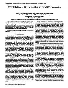
Fig. 1. Distributed transmission line model.
VR + Z c I R γ x VR − Z c I R −γ x ⎧ e + e ⎪⎪V = 2 2 ⎨ ⎪ I = VR / Z c + I R eγ x − VR / Z c − I R e−γ x ⎪⎩ 2 2
modeling of an ac line can be somehow simplified to represent the transient characteristics of fundamental frequency only, while ignoring other frequency spectrum.
(1)
where, Z c = L / C , γ = ( R + jωL)(G + jωC ) . Zc is the characteristic impedance and γ is the propagation constant, which is frequency dependent. L and C are inductance and capacitance in per unit length.
Alternatively and also in practice, it is more convenient to use an equivalent circuit to analyze the transmission line. This leads to the lumped parameter line model, which represents the performance of the line seen from its terminal. Again as shown in (1), this model is also frequency dependent. However, for short lines and medium lines (shorter than 250 km), the impact of the frequency term on line impedance is trivial, resulting in the frequency independent short/medium line models. This renders the hardware emulation of ac line easier. Conceptually, BTB converters can control the two ends currents or power, so that they can behave as an ac transmission line. In terms of hardware implementation, e.g. Bergeron’s model, the time domain current and voltage information in one end needs to be transmitted to the other end, which causes evident communication delay and could possibly distort the propagation characteristics of the long line model, giving the fact that propagation delay of current traveling wave is only around 300~400 μs. Even for the short line model, the inevitable communication delay could also cause an undesired angle delay at two ends current, considering that 46 μs corresponds to one degree in 60 Hz systems.
On the other hand, if looking into the physics of an ac line from the power flow perspective as shown in Fig. 2, ac line provides a direct path for active power flow, and also a storage tank to absorb in and transfer out the energy in the form of reactive power. If the terminal active and reactive power of the emulation converters can be controlled exactly the same as that in the real ac line, then the emulation objective can be obtained. V1∠δ
I AC
Lf
Lf
ia ib ic
Fig. 2. Concept of BTB ac line emulation in phasor domain.
Thus, a simplified emulation model from this power flow perspective is proposed. First, a suitable pi model is selected and directly used to calculate the line impedance at 60 Hz. Initially, a short lossless line model is selected for emulation at the time being. Then, adopting the measured voltage at the sending and receiving ends, the transmitted active and reactive power is calculated to control the BTB converters. A typical short line model [12] is illustrated in Fig. 3. V2 ∠0
V1∠δ
In this paper, the focus will be on the hardware emulation implementation strategy of the short line model as the starting point. Two approaches respectively in phasor domain and time domain are proposed. The emulation principle, advantages, and limitations are discussed in section II. Corresponding control schemes are implemented under d-q coordinates instead of static coordinates [4, 11] are presented in section III, which effectively mitigates the demanding requirement for fast communication speed between BTB converters. Finally, the impacts of BTB converter losses on emulation performance are investigated and improved after applying an extra dc power supply. Simulation and experimental results are given in section IV. II.
V2 ∠0
X
Fig. 3. Equivalent pi model of the single phase long line
⎧V1 = cosh(γ l ) ⋅V2 + Z c sinh(γ l ) ⋅ I 2 ⎪ sinh(γ l ) ⎨ ⋅V2 + cosh(γ l ) ⋅ I 2 ⎪ I1 = Z c ⎩ ⎧V1 = cosh(γ l ) ⋅V2 + Z c sinh(γ l ) ⋅ I 2 ⎪ sinh(γ l ) ⎨ ⋅V2 + cosh(γ l ) ⋅ I 2 ⎪ I1 = ⎩
MODLEING EMULATION OF AC LINE
(2)
(3)
Zc
The matrix form can also be obtained as
A. Phasor Domain Modeling and Emulation As mentioned above, the time domain based modeling approach such as Bergeron model can accurately represent the dynamic response of line voltage and current if the discrete step size is small enough. However, in many cases of power system study, the transients related to voltage magnitude, power angle oscillation are slow, and line impedances are calculated only based on fundamental frequency, as some commercial software has done. This indicates that the
⎡V1 ⎤ ⎡ A B ⎤ ⎡V2 ⎤ ⎢ I ⎥ = ⎢C D ⎥ ⎢ I ⎥ ⎦⎣ 2⎦ ⎣ 1⎦ ⎣
(4),
where l is the line length, and A = cosh(γ l )
B = Z c sinh(γ l )
sinh(γ l ) C= Zc
D = cosh(γ l )
(5)
Then, the active and reactive power at the two ends can be derived as [12]
1808
⎧ 3 A V12 cos(θ B − θ A ) 3V1V2 cos(θ B + δ ) − ⎪ P1 = B B ⎪ ⎨ 2 ⎪Q = 3 A V1 sin(θ B − θ A ) − 3V1V2 sin(θ B + δ ) ⎪ 1 B B ⎩ 2 ⎧ 3V1V2 cos(θ B − δ ) 3 A V2 cos(θ B − θ A ) − ⎪ P2 = B B ⎪ ⎨ 2 3 A V sin( θB −θ A ) − 3 V V sin( θ δ ) ⎪Q = 1 2 2 B − ⎪ 2 B B ⎩
(6)
(7).
where θA and θB are the angle of A and B in polar form, and δ is the power angle between the two ends. Initially, a short lossless line model is selected for emulation at the time being. From (6) ~ (7), the power reference at two ends can be simplified as 3V V sin δ (8) P= 1 2 P=P 1
1
X 3V1 (V1 − V2 cos δ ) ⎧ Q = ⎪⎪ 1 X ⎨ ⎪Q = 3V2 (V1 cos δ − V2 ) ⎪⎩ 2 X
2
(9).
B. Time Domain Modeling and Emulation Different from the phasor domain model, the time domain model is more suitable for power system stability and transient study. For example, if a short line model is simplified as an inductance, it follows diSR (t ) vS (t ) − vR (t ) (10). = dt L Trapezoidal discrete method then can be applied for this time domain model to avoid possible numerical instability when digitally implemented [4, 10].
τ [vS (k ) + vS (k −1) − vR (k ) − vR (k − 1)] + iSR (k − 1) (11) 2L where τ is the discrete step size, and “S” “R” denote the sending end and receiving end. C. Dynamic Performance and Limitation As shown in (8) and (9), although line impedance X is calculated at fundamental frequency, it does not mean this proposed modeling approach is only valid at the steady state. On the other hand, contributed by the real-time measurement and phase-locked-loop (PLL), voltage magnitude can be tracked and updated cycle by cycle. Similarly, the power angle is also updated by PLL in each fundamental cycle. Consequently, the power reference could be updated in the same speed and enables this emulation system to represent the transient characteristics of power flow along the transmission line in the range of tens of Hz. iSR (k ) =
III.
CONTROL IMPLEMENTATION
A. Control Scheme of Phasor Domain Model The control structure of BTB emulation is presented in Fig. 4 with a master-slave configuration. The ac line model is implanted inside the inverter, while the rectifier receives the reactive power reference Q2 from the inverter side. Ideally, if the power loss of BTB voltage source converters is negligible, by controlling the dc link voltage at the rectifier side, the active power balance could be automatically achieved, thus no communication of active power reference P2 is required. Each VSC is controlled under d-q coordinates, and synchronized with the grid voltage by PLL. To calculate the power reference in (8) and (9), the rectifier side voltage and angle need to be sent to the inverter side controller. Different from the time domain static coordinate approach, the voltage and power signal are dc components, being relatively insensitive to the communication delay. This mechanism eliminates the time delay effects in steady state, reduces the error in power reference calculation, and also sets an example for the accurate emulation of the time domain model. P1 Q1
P2 Q2
Vd 2
δ2 VDC *
Q2
Q2
P1 Q1
Fig. 4. Control scheme of BTB emulation in Phasor Domain.
B. Power Angle Calculation The power angle cannot be easily acquired. As shown in (8), it is determined by the difference of the two ends voltage angle and is very sensitive for the power calculation. If using the common digital protocols to send the rectifier side angle δ2, the estimated delay could be around 100 μs, depending on the microcontroller and protocol, which could lead to an angle delay of more than 2 degrees. A dedicated digital approach is proposed in Fig. 5. One pulse synchronized with its PLL angle is produced from the rectifier DSP and sent to the inverter side DSP through digital IO. By detecting the edge of this pulse and identifying its leading/lagging status, the inverter side controller can determine the power angle between the two ends.
Time domain emulation model on the other hand, is more sensitive to communication or control delay, but better represents the transient at the frequency ranges which are generally enough for the common power system studies, such as frequency control, voltage control, and transient stability study.
Fig. 5. Power angle calculation method 1.
1809
However, due to the mismatch between the instants of inverter control interruption and the rising edge of the cycle pulse, there is still certain detection delay, up to one PWM period, i.e. 50 μs in this paper. To deal with it, one digital solution is illustrated in Fig. 6. δ1 is the rectifier side angle at the edge of the pulse, and δ2 is the detected angle at the inverter side control interruption. The basic idea is to compensate this arbitrary delay by introducing an IO interrupt with the highest priority for this pulse in the inverter side DSP. The digital compensation can be achieved by timing the inner DSP counter between the edge of the pulse and the interruption instant, as shown in (12). With this, the accuracy of power angle is ensured and the angle delay is avoided.
Ideally, if there is no loss, one obtains the active/reactive power at two ends 3V V sin δ 3 (16) P1 = 1 2 = Vd 1 I d 1 2 X 3 (17) Q1 = 3V1 I AC sin(δ + θ ) = − Vd 1 I q1 2 3V V sin δ 3 (18) P2 = 1 2 = Vd 2 I d 2 2 X 3 (19), Q2 = 3V2 I AC sin θ = − Vd 2 I q 2 2 where, two converters are synchronized with their local grid voltage and the control is implemented under each rotated d-q frame.Vd1, Vd2, Vq1, and Vq2 are the voltages under d-q frame, Id1, Iq1, Id2, and Iq2 are the currents under d-q frame. Substituting (13) ~ (15) into (16) ~ (17), the sending side current can be obtained as ⎧ 2V2 sin δ = 2 I AC cos(δ + θ ) ⎪ I d1 = (20), X ⎨ ⎪ I = − 2 I sin(δ + θ ) AC ⎩ q1
which means the controlled current at sending side converter is the desired line current.
JG JJJG I1 = I AC ∠δ + θ = I AC
Fig. 6. Improved power angle calculation method
δ1 = δ 2 − Δδ
(12) where, δ1 is the rectifier side angle at the edge of the pulse, and δ2 is the detected angle at the inverter side control interruption. C. Emulation Feasibility and Loss Impacts of BTB To further investigate the validity, in this section, the feasibility of this emulation scheme and its limitation when considering the actual loss in BTB converters, are analyzed. For a lossless line, its single line diagram and phasor relationship are illustrated in Fig. 7 and Fig. 8, respectively. Three geometrical relations are obtained, as given in (13) ~ (15). Vg 2 ∠0 Vg1∠δ X I AC
Fig. 7. One line diagram of two ends transmission line.
V1 δ
θ
I AC
V2
(21) Similarly, the receiving end current can also be controlled the same as the line current in (22) ~ (23), which indicates the currents flowing in and out of the AC lines are in phase and the short line mode is well emulated.
⎧ 2V1 sin δ = 2 I AC cos θ ⎪Id 2 = X ⎨ ⎪ I = − 2 I sin θ AC ⎩ q2
JJG JJJG I 2 = I AC ∠θ = I AC
(23) However, in this BTB emulator, the ac power balance is ensured by rectifier dc voltage control. If considering the converter loss, active power transferred by the rectifier will be reduced by ∆P, as shown in (24). 3V V sin δ 3 (24) P2 = 1 2 − ΔP = Vd 2 I d 2 2 X Correspondingly, the current at d axis reduces (25) and rectifier side current I2 tends to be leading the desired current IAC by ∆θ while its magnitude gets smaller, as demonstrated in Fig. 9. The red dotted line denotes the real current, and blue dotted line represents the desired current. ⎧ 2V1 sin δ 2 sin δ − = I d 2 _ r − ΔI d 2 < 2 I AC cos θ (25) ⎪Id 2 = X 3V2 ⎨ ⎪ I = − 2 I sin θ AC ⎩ q2
V1∠δ
Fig. 8. Phasor relationship between two ends.
V1 sin δ = I AC X cos θ V1 cos δ − V2 = I AC X sin θ
(13)
V2 sin δ = I AC X cos(δ + θ )
(15)
(22)
(14)
1810
I AC
δ
V2 ∠0 Fig. 9. Impact analysis of power loss at receiving end.
The angle leading at receiving end (rectifier side) is given in (26) and (27). As illustrated in Fig. 10, the angle delay introduced by the converter loss is almost linearly increasing as the losses rise. Based on the test set-up parameter shown in Table I, it is typically less than 1 degree, assuming a loss lower than 10%.
ΔI ΔP ΔP = = d2 P1 P2 + ΔP I d 2 _ r
Δθ = arctan
Iq2 I d 2 _ real
− arctan
three-phase line currents emulated in abc frame are transferred to d-q frame based on the respective PLL angle before sending out to the slave controller. Also, both ends current control are directly implemented under d-q frame. This control scheme also ensures the possibility to accurately emulate the long line propagation constant if Bergeron’s model is implemented.
(26)
Iq2
Lf
Lf
(27)
Id 2 _ r
Angle Leading v.s. Converter Loss
Angle Leading (degree)
2.5 2 1.5 1 * idq _ S ( k ) = TS iSR ( k )
0.5 0
* idq _ R (k ) = TR iSR (k )
Fig. 12. Control scheme of time domain line emulation. 0
0.05
0.1
0.15
0.2
IV.
Ratios of Converter Loss Fig. 10. Angle leading in vs. power loss.
For more accurate power flow control, this angle delay should be eliminated. A simple solution is to compensate the converter loss by an extra dc source which provides the loss power, as shown in Fig. 11. With that, BTB converters can fully control the active and reactive power. In addition, this new configuration can also emulate the line loss precisely. DC Bus
VDC
G
G
208V
208V
Area 1
Area 2
Fig. 11. Improved emulator configuration: BTB plus an extra dc source.
D. Control Scheme of Time Domain Model Fig. 12 shows the control block diagram. Similar to the phasor domain scheme, here the receiving end controller is selected as the master controller where the time domain model is emulated. As shown in (11), the three-phase sending end voltages are needed for line current calculation. And the current references also need to be sent from the master controller to the slave controller “simultaneously”. To reduce the communication delay, the salve controller side ac voltages sampling signals are shared with the master controller. Thus, only the current references communication is required. RS232 serial protocol is used for convenience. To further suppress the delay effects, the concept of d-q frame communication instead of abc frame is adopted again. That is to say, the references of
SIMULATOIN AND EXPERIMENTAL VERIFICATION
A. Simulation Test Comparisons among the ac short lossless line and two BTB emulation schemes are conducted in Matlab/Simulink. To ensure currents are well damped to ac operating point after transients, external ESR with X/R = 0.1 are inserted. Fig.13 shows the comparison with the phasor domain model. Two scenarios are studied. First, in the line tripping scenario, assuming one set of the two paralleled three-phase ac lines is tripped at t = 0.2s, line impedance increases to 1.5 p.u. Then, in the voltage disturbance scenario, line voltage increases to 1.2 p.u. at t = 0.3s, and returns back to its rated value at t = 0.4s. In both scenarios, the ac currents at the sending and receiving end VSCs show the same magnitude and phase angle as the ac line current in the detailed model, not only in the steady state but also during the transients. Also the emulator currents are almost the same as that of the ac line. However, since the phase domain model is based on the quasisteady state equations, the dc current bias during the transient with damping time constant X/R is not reflected in the emulation model. This mismatch with Simulink line model can be clearly seen in start-up and step change transients. Similarly, Fig. 14 gives the comparison with the time domain emulation model. As we can see, the time domain based emulation presents almost the same transient characteristics as Simulink inductor model does.
1811
Fig. 15. Prototype of the scaled down BTB emulator.
A lossless short line is implemented in this BTB emulator and different implementation strategies are compared.
Fig. 13. Currents of ac line and BTB phasor domain emulation. (A) 30
Ia X=1.5 p.u.
X=1 p.u.
20
V1=1.2 p.u.
Originally, with the proposed control scheme and power angle calculation method in Fig. 5, the two end ac currents are almost in phase and the emulator behaves similarly to an ac inductor, as shown in Fig 16. However, the rectifier (receiving end) current leads the inverter side current by 2~4 degrees (200μs) as shown in Fig. 17. The amplitude of the rectifier side current is about 1.7A lower than that in the inverter side.
V1=1 p.u.
10 0 -10 -20 -30
(A)
Ib
40 30 20 10 0 -10 -20
(A)
iinv A (10A/div)
irec A (10A/div)
vinv
vrec
AB
(100V/div)
AB
(100V/div)
Ic
30 20 10 0 -10 -20 -30 0
0.05
0.1
0.15
0.2
0.25 Time (s)
0.3
0.35
0.45
0.5
Receving VSC
Sending VSC
AC line
0.4
Fig. 14. Currents of ac line and BTB time domain emulation.
B. Experimental Results of Phasor Domain Model To verify the emulation scheme, a scaled-down BTB system is implemented experimentally, as shown in Fig. 15. The main parameters are summarized in Table I. To mimic the power angle in the laboratory setup, a Y/∆ transformer is introduced to provide a 30 degree phase shift of the grid voltage.
Fig. 16. Ac voltages and currents at two ends.
TABLE I SYSTEM PARAMETERS Parameters
Values
Sending grid voltage
90 V (30 degree leading by Y/∆)
Receiving grid voltage
85 V ( 0 degree)
Line inductance Dc link voltage
5 mH
Dc reactors
150 V 0.5 mH
Fig. 17. Phase difference between two end currents.
1812
Fig. 20. Ac voltages and currents at two ends with improved emulation configuration: BTB plus the extra dc source.
After adopting the improved power angle calculation method, the power angle error is reduced to be around 84 μs (less than 2 degrees) and the magnitude difference in two end currents is 1.2 A, as seen in Fig. 18 and Fig. 19.
iinv A (10A/div)
irec A (10A/div)
vinv
vrec_AB (100V/div)
AB
(100V/div)
Fig. 21. Phase difference between two end currents with improved emulation configuration: BTB plus the extra dc source.
To verify the transient performance of the line emulation, a line tripping scenario is tested. Fig. 22 shows the experimental results when the line impedance has a step change from 5mH to 7mH if assuming one of the two paralleled lines is tripped. It can be observed that the two ends currents change smoothly during the event within one cycle, maintaining the same magnitude and phase angle. Yet, it is also noticed that some transient oscillations due to step change of line inductance are not reflected due to the quasi-steady state nature of this phasor domain model.
Fig. 18. Ac voltages and currents at two ends with improved power angle calculation scheme.
Fig. 19. Phase difference between two end currents with improved power angle calculation scheme.
Fig. 20 and Fig. 21 show the results after introducing the additional dc power supply. With independent power control in both converters, the magnitudes of the two end currents are almost the same and the phase shift between them is close to 0.16 degree (8 μs). Considering the measurement error, these results verify the analysis of power loss impact and the feasibility of the whole BTB emulation schemes.
iinv A (10A/div)
irec A (10A/div)
vinv
vrec
(100V/div) AB
(100V/div) AB
Fig. 22. Ac line tripping scenario with improved emulation configuration: BTB plus the extra dc source.
C. Experimental Results of Time Domain Model Although the steady state performance of the time domain emulation model is similar to that of the phasor domain model, its transient performance is still to be verified. A system study is carried in HTB emulation platform, as shown in Fig. 23, which is a scaled-down Kundur two area system. The BTB emulator is compared with three 7.5 mH physical inductors. A 0.1 p.u. step change of load power is set in the transient test, where generator G1, G4 and load L9 are activated. Results of active power and frequency of G1 in two cases are given in Figs. 24 and 25, where Pind and find denote the power and frequency with inductors, and Pemu and femu are the power and frequency with the line emulator. The shapes of transient
1813
oscillation waveforms in both cases are quite close, while the minor mismatch may come from the measurement error in inductance value and ESR value of the inductors. DC Bus G1
Short Distance Transmission Line Emulator
Short Distance Transmission Line Emulator
DC Bus
DC Bus G3
G2
Long Distance Transmission Line Emulator based on BTB
G4
L7
2.5mH*3
L9
Area 1
Output Inductors
2.5mH
2.5mH
Long Distance Transmission Line Emulator
Output Inductors
Area 2
Fig. 23. Schematic of HTB two-area systems.
G1 active power
P (p.u.)
0.25 0.2
ACKNOWLEDGMENT
Pind
0.1 0
10
20 Time (s)
30
CONCLUSION
The emulation schemes for the BTB power converter based ac transmission line emulation are proposed with regard to different line models. This phasor domain model can represent the transient characteristics of ac line events below fundamental frequency, while the time domain model shows better transient capability. The implementation strategy is also presented which is immune against the time delay, thus mitigating the fast requirement for communication speed. The feasibility of BTB emulation is theoretically proved, only showing inaccuracy when considering the loss impacts of BTB converters and the loss line. With an extra dc source/bus, this hardware configuration can fully represent the loss lines. Simulation and experimental results obtained from a prototype well verify the feasibility and control accuracy of the ac line emulation, showing the good steady state and dynamic performance under normal operation and line tripping scenarios.
Pemu
0.15
0.05
V.
40
This work was supported primarily by the Engineering Research Center Program of the National Science Foundation and Department of Energy under NSF Award Number EEC1041877 and the CURENT Industry Partnership Program.
G1 active power P (p.u.)
0.25
REFERENCES
Pemu
0.2
[1]
Pind
0.15 0.1 0.05
0
10
20 Time (s)
30
40
Fig. 24. Active power flow during power step up and down transients.
G1 frequency freq (Hz)
60.5
femu find
60 59.5 59
0
10
20 Time (s)
30
40
30
40
G1 frequency freq (Hz)
60.4 femu
60.2
find
60 59.8 59.6
0
10
20 Time (s)
Fig. 25. Frequency during power step up and down transients.
M. O. Faruque and V. Dinavahi, “Hardware-in-the-loop simulation of power electronic systems using adaptive discretization,” IEEE Trans. Ind. Electron., vol. 57, no. 4, pp. 1146–1158, Apr. 2010. [2] J. Wang, L. Yang, Y.W. Ma, X.J. Shi, X.H. Zhang, L.J. Hang, K.M. Lin, L. M. Tolbert, F. Wang, and K. Tomsovic, “Regenerative Power Converters Representation of Grid Control and Actuation Emulator,” in Proc. IEEE APEC, 2012, pp. 2460-2465. [3] L. Yang, Y.W. Ma, J.X. Wang, J. Wang, X.H. Zhang, L. M. Tolbert, F. Wang, and K.Tomsovic, “Development of Converter Based Reconfigurable Power Grid Emulator,” in Proc. IEEE ECCE, 2014, pp. 3990-3997. [4] H. W. DOMMEL, “Digital Computer Solution of Electromagnetic Transients in Single- and Multiphase Networks,” IEEE Trans. Power App. and Sys., vol. PAS-88, no. 4, pp. 388-399, Apr. 1969. [5] R.C. Silva, S. Kurokawa, E.C.M. Costa, and J. Pissolato, “Development of A Simplified Transmission Line Model Directly in the Phase Domain,” in Proc. IEEE PESGM, 2012, pp. 1-8. [6] M. Chanaka, S. Kusum, and P. Ranjit, “Modeling of Power Transmission Lines for Lightning Back Flashover Analysis (A Case Study: 220kV Biyagama-Kotmale Transmission Line),” in Proc. IEEE ICIIS, 2011, pp. 386-391. [7] M. Taleb, M.J. Ditto, and T. Bouthiba, “Performance of short transmission lines models,” in Proc. IEEE GCC, 2006, pp.1-7. [8] B. Gustavsen, “Frequency Dependent Transmission Line Modeling Utilizing Transposed Conditions,” in IEEE Trans. Power Delivery, vol. 17, no. 3, pp. 834-839, Jul. 2002. [9] B. Asghari and V. Dinavahi, “Real-Time Nonlinear Transient Simulation Based on Optimized Transmission Line Modeling,” IEEE Trans. Power Sys., vol. 26, no. 2, pp. 699-709, May 2011. [10] H.V. Nguyen, H.W. Dommel, and J.R. Marti, “Modeling of Singlephase Non-uniform Transmission Lines in Electromagnetic Transient Simulations,” IEEE Trans. Power Delivery, vol. 12, no. 2, pp. 916-921, Apr. 1997. [11] R.B. Canonico, V.A.F. Silva, A.J. Prado, S. Kurokawa, and L.F. Bovolato, “Simulations of electromagnetic transients in a transmission line using state variables,” in Proc. IEEE TDC-LA, 2008, pp. 1-7. [12] H. Saadat, Power System Analysis (2nd Ed.), McGraw-Hill, 2002.
1814