Control of Autonomous Linear Systems. M403 Lecture Notes by Philip D. Loewen
. We study systems governed by the controlled differential equation. ˙x(t) = Ax(t) ...
Control of Autonomous Linear Systems M403 Lecture Notes by Philip D. Loewen We study systems governed by the controlled differential equation x(t) ˙ = Ax(t) + Bu(t),
x(0) = ξ,
(∗)
where x evolves in Rn , u evolves in Rm , and the coefficient matrices A ∈ Rn×n and B ∈ Rn×m are given. We will focus primarily on the class of piecewise continuous control functions u: a function u: [0, +∞) → Rm is called piecewise continuous if every finite interval [0, b] admits a finite partition 0 = a0 < a1 < . . . < aN = b with the property that u is continuous on each open interval (ak−1 , ak ) with finite − one-sided limits u(a+ k−1 ) and u(ak ) for each k = 1, 2, . . . , N . The collection of all piecewise continuous functions is denoted P WC. Recall that for a fixed control u in P WC, the unique solution of (∗) is given by Z t tA e(t−r)A Bu(r) dr. x(t) = e ξ + 0
(The right-hand side of this formula actually makes sense for any function u that is integrable on every finite real interval.) We will look at three different approaches to the choice of u in (∗), each with different criteria and outcomes: linear feedback and eigenvalue assignment, linearquadratic regulator design, and time-optimal control. A. Controllability Introduction. Which states can be joined by a piecewise continuous control function? To answer this basic question, consider the attainable set � � Z t A(t−r) m n At e Bu(r) dr for some u ∈ P WC ([0, t]; R ) . A(t; ξ) = η ∈ R : η = e ξ + 0
This set contains a point η if and only some Rm drives the state to the terminal point η system equation (∗) starting from x(0) = ξ. subset of Rn . At least three of its properties
piecewise continuous control u: [0, t] → at time t, along a trajectory x for the In general, A(t; ξ) is a time-dependent are comparatively obvious:
(i) A(t; ξ) = eAt ξ + A(t; 0), for all t ≥ 0, ξ ∈ Rn ;
(ii) A(t; 0) is a linear subspace of Rn for every t ≥ 0;
(iii) A(t; ξ) is an affine subspace of Rn for every t ≥ 0. We can characterize A(t; ξ) with the aid of line (i) and the famous controllability matrix � � C := B | AB | A2 B | · · · | An−1 B .
This is an n × mn matrix formed by stacking n matrices of size n × m side by side; examples appear below. File “linsys”, version of 19 Jan 2010, page 1.
Typeset at 12:14 September 17, 2012.
2
PHILIP D. LOEWEN
A.1. Theorem. For each t > 0, one has (a) A(t; 0) = Im(C) = {Cw : w ∈ Rnm }; � (b) A(t; 0)⊥ = ker(C T ) = y ∈ Rn : C T y = 0 ; and (c) dim A(t; 0) = rank(C).
Proof. For any matrix C, standard results from linear algebra assert that Im(C)⊥ = ker(C T ) and rank(C) = dim(Im(C)). Consequently (a) implies both (b) and (c). But since one has (S ⊥ )⊥ = S for every subspace S of Rn , it is also true that (b) implies (a). Thus the theorem can be established simply by proving (b). This we now do. (b)(⊇) If y is a vector in ker(C T ), then C T y = 0, so � � 0T = y T C = y T B | y T AB | y T A2 B | · · · | y T An−1 B .
(Both sides here are row vectors of size mn.) Now by the Cayley Hamilton theorem, A satisfies its own characteristic polynomial. That is, for the coefficients a0 , . . . , an−1 defined by p(s) = det(sI − A) = sn − an−1 sn−1 − . . . − a1 s − a0 , the following matrix equation holds: 0 = p(A) = An − an−1 An−1 − . . . − a1 A − a0 I. In particular, one has An = an−1 An−1 + . . . + a1 A + a0 I, and it follows that ! n−1 n−1 X X � i T n T ai y T Ai B = 0. ai A B = y A B=y i=0
i=0
Likewise, y T Ak B = 0 for all k ≥ 0. It follows that for any r ∈ [0, t], one has ! N k X (t − r) lim y T e(t−r)A B = y T Ak B N→∞ k! k=0 � � N N X (t − r)k X T k = lim 0 = 0. (y A B) = lim N→∞ N→∞ k! k=0
k=0
It follows that for any control u in P WC, one has Z t T e(t−r)A Bu(r) dr, 0=y 0
which shows that 0 = y T η for every η ∈ A(t; 0). This is the definition of y ∈ A(t, 0)⊥.
(b)(⊆) If y is a vector in A(t; 0)⊥, then 0 = y T η for every η ∈ A(t; 0). In other words, for any control u in P WC, one has Z t T eA(t−r) Bu(r) dr, 0=y 0
File “linsys”, version of 19 Jan 2010, page 2.
Typeset at 12:14 September 17, 2012.
Control of Autonomous Linear Systems
3
T
Choosing the control u(r) = B T eA (t−r) y reveals Z t T (t−r)A 2 0= B dr, y e 0
from which we deduce that y T eA(t−r) B = 0 for all r in [0, t]. Alternately letting r → t and differentiating in this relation, we have ! y T eA(t−r) B = 0
∂ : ∂r
y T eA(t−r) (−A)B = 0
∂ : ∂r
y T eA(t−r) (−A)2 B = 0
∀r ∈ (0, t)
⇒ yT B = 0
∀r ∈ (0, t)
⇒ y T AB = 0
∀r ∈ (0, t)
⇒ y T A2 B = 0
!
!
.. . ∂ : ∂r
y T eA(t−r) (−A)n−1 B = 0 ∀r ∈ (0, t)
⇒ y T An−1 B = 0
!
� � This reveals that 0T = y T B | y T AB | · · · | y T An−1 B = y T C, i.e., C T y = 0.
////
A.2. Corollary. For a given pair of matrices A ∈ Rn×n and B ∈ Rn×m , the following assertions are equivalent: � � (a) rank(C) = n, where C = B | AB | · · · | An−1 B ; (b) A(t; 0) = Rn for some t > 0. (c) A(t; 0) = Rn for each t > 0.
(d) A(t; ξ) = Rn for each t > 0 and each ξ ∈ Rn . In this case we say the matrix pair (A, B) is controllable. A.3. Remarks. (a) If the pair (A, B) is uncontrollable, then any trajectory of (∗) starting from the origin is trapped in the fixed subspace A(t; 0) = Im(C) of Rn for all time. Any trajectory starting from some initial point ξ can never leave the moving affine subspace A(t; ξ) = eAt ξ + Im(C). (b) In situations where the main goal is to stabilize the system, a more intuitive notion is null-controllability: one defines N (t) = {ξ ∈ Rn : 0 ∈ A(t; ξ)} as the set of all initial points that can be steered to the origin by some control acting on the interval [0, t]. But we note that ξ ∈ N (t) ⇔ 0 ∈ eAt ξ + A(t; 0) ⇔ ξ ∈ −e−At A(t; 0).
It follows that N (t) = −e−At A(t; 0) is a subspace of Rn for each t > 0. In fact, it is a constant subspace, equal to A(t; 0) = Im(C) for all t > 0. (This is a nice practice problem.) File “linsys”, version of 19 Jan 2010, page 3.
Typeset at 12:14 September 17, 2012.
4
PHILIP D. LOEWEN
(c) Theorem A.1 remains valid for various families of control functions u beyond the collection of piecewise continuous controls: we could use only continuous controls, or we could permit only piecewise constant controls. The key to the proofs above is to have a vector space U of control functions sufficiently large that y T η = 0 for all η ∈ A(t; 0) will imply y T eA(t−r) B = 0 for all r ∈ [0, t]. Any one of the three just mentioned has this property. (d) The equation A(t; 0) = Rn for all t > 0 is mathematically correct, but clearly unrealizable in practice. This inconsistency reveals a flaw in the modelling behind (∗), which allows for arbitrarily large values for the control input vector u. Later we will see how putting constraints on u changes the picture. (e) If m < n you can save time by computing A(AB) instead of (A2 )B, even though the two results are equal. A.4. Examples. (a) A system trapped in the plane z = 0. 0 1 0 0 0 | A = 1 0 0, B = 1 =⇒ C = 1 | 0 0 1 0 0 |
1 | 0 0 | 1. 0 | 0
This system is not controllable, because the columns of C span only a 2-dimensional subspace of R3 : r A(t; 0) = Im(C) = s : r, s ∈ R . 0 (b) Linearized satellite problem. Here
0 3ω 2 A= 0 0
1 0 0 −2ω
0 0 0 2ω , 0 1 0 0
0 0 B= 0 1
0 1 . 0 0
Computation gives
0 0 C= 0 1
0 1 0 0
| 0 | 2ω | 1 | 0
1 0 0 −2ω
| 2ω | 0 | 0 | −4ω 2
0 −ω 2 −2ω 0
| 0 | −2ω 3 | −4ω 2 | 0
−ω 2 0 . 0 2ω 3
The first 4 × 4 block has full rank, so the system is controllable. Loss of radial thrust: If motor failure forces u2 ≡ 0, this is the same as setting column 2 of matrix B to zero. This will zero columns 2,4,6,8 of matrix C, but the rank will still be 4, so the system remains controllable. Loss of tangential thrust: If instead we set column 1 of matrix B to zero, this zeros columns 1,3,5,7 of matric C and reduces its rank to 3. (row 4 is a multiple of row 1). Controllability is broken. //// File “linsys”, version of 19 Jan 2010, page 4.
Typeset at 12:14 September 17, 2012.
Control of Autonomous Linear Systems
5
B. Linear State Feedback Consider this linear time-invariant (LTI) system in which a scalar input u drives a scalar response variable x through a differential equation of order n: x(n) + an−1 x(n−1) + an−2 x(n−2) + . . . + a2 x ¨ + a1 x˙ + a0 x = u.
(∗)
There are two approaches to controlling it. The first is open-loop control, where we use prior knowledge of the initial system configuration to design a particular function u = u(t) for use in (∗). Different initial conditions will typically require a completely different function u. In the second approach, closed-loop control, we design a function U : Rn → R and use it to generate the input signal in (∗) by enforcing the identity u(t) = U (x(t), x(t), ˙ . . . , x(n−1) (t)). This is mathematically equivalent to replacing (∗) with the autonomous dynamical system x(n) + an−1 x(n−1) + . . . + a2 x ¨ + a1 x˙ + a0 x = U (x, x, ˙ . . . , x(n−1) ).
(†)
Ideally, the feedback law U could be chosen so that the closed-loop system has good dynamics independent of the choice of initial data. The simplest type of feedback function U is linear: we choose constants f0 , f1 , . . . , fn and specify U (x1 , x2 , . . . , xn ) = f0 x1 + f1 x2 + · · · + fn−1 xn .
With this choice, system (†) becomes
x(n) + an−1 x(n−1) + . . . + a2 x ¨ + a1 x˙ + a0 x = f0 x + f1 x˙ + f2 x ¨ + . . . + fn−1 x(n−1) , x(n) + (an−1 − fn−1 ) x(n−1) + . . . + (a2 − f2 ) x ¨ + (a1 − f1 ) x˙ + (a0 − f0 ) x = 0. (‡)
To solve (‡) would involve “guessing” x = est and plugging in, then observing that we have a solution if and only if the complex constant s obeys def
0 = p(s) = sn + (an−1 − fn−1 ) sn−1 + . . . + (a2 − f2 ) s2 + (a1 − f1 ) s + (a0 − f0 ) .
Since the constants fk are our design parameters, we can influence every coefficient in this polynomial, and hence arrange any collection of zeros we want for the characteristic polynomial. (The only restriction is that since p is a polynomial with real coefficients, its zeros must occur in complex-conjugate pairs.) In detail, given any set of n complex numbers λ1 , λ2 , . . . , λn with reflection symmetry across the real axis of the complex plane, a polynomial with these numbers as its zeros is given by P (s) = (s − λ1 )(s − λ2 ) · · · (s − λn ) = sn + αn−1 sn−1 + · · · + α2 s2 + α1 s + α0
for suitable real constants α0 , . . . , αn . (Knowing the λk ’s lets us compute the αk ’s.) We can arrange for the zeros of p to fall at precisely these points by forcing p ≡ P , i.e., by choosing a k − fk = α k ,
or fk = ak − αk , k = 0, 1, . . . , n − 1.
Practically-minded people (e.g., engineers) have pretty clear ideas of what regions in the complex plane make good homes for the eigenvalues for a well-behaved system. We explore these next. File “linsys”, version of 19 Jan 2010, page 5.
Typeset at 12:14 September 17, 2012.
6
PHILIP D. LOEWEN
Eigenvalue Assignment Criteria. We use the simplest possible 2 × 2 system to justify some standard design criteria used in applied science. Suppose we choose the feedback matrix F and apply it, to obtain an autonomous system with coefficient matrix � � 0 1 A + BF = . −ω 2 −2ζω (Here ζ ∈ [0, 1) is the “damping factor” and ω > 0 is the “undamped natural frequency”, both constant.) Study desirable properties of solutions to x˙ = (A + BF )x, starting with an expansion of x(t) = (y(t), v(t)): y˙ = v,
v˙ = −ω 2 y − 2ζωv
y¨ + 2ζω y˙ + ω 2 y = 0.
=⇒
Guess y = est for constant s and get solutions iff p p 0 = s2 + 2ζωs + ω 2 , i.e., s = −ζω ± ζ 2 ω 2 − ω 2 = −ζω ± iω 1 − ζ 2 .
(Or, look for eigenvalues of A + BF using its characteristic polynomial, which can be read out of the matrix directly, thanks to its special form (treated last class): p(λ) = λ2 + 2ζωλ + ω 2 . The same complex numbers result.) Running the system x˙ = (A + BF )x from the initial state x(0) = (1, 0) produces a trajectory whose first component is # " p p ζ sin( 1 − ζ 2 ωt) . (1) y(t) = e−ζωt cos( 1 − ζ 2 ωt) + p 1 − ζ2 We study y using the change of variables θ = ωt, writing " # p p ζ sin( 1 − ζ 2 θ) . Y (θ) = y(θ/ω) = e−ζθ cos( 1 − ζ 2 θ) + p 1 − ζ2
The sketch below shows Y for ζ = 12 .
1 0.8 Y=Y(θ) for ζ=1/2
0.6 0.4 0.2 0 −0.2 −0.4
0
2
File “linsys”, version of 19 Jan 2010, page 6.
4
6
8
10
12
Typeset at 12:14 September 17, 2012.
Control of Autonomous Linear Systems
7
Standard methods reveal that ! � � p 1 ζ −ζθ −1 p Y (θ) = e cos( 1 − ζ 2 θ − φ) for φ = tan . (2) 1 − ζ2 1 − ζ2 � � 1 The decaying exponential factor 1−ζ e−ζθ is also shown in the sketch above. Three 2 desirable properties can be quantified with reference to this figure. Response Time. Write tR for the time required for the disturbance applied above to make the transition from 90% of its initial height to 10%. That is, ωtR = θ2 −θ1 =: θR for the smallest positive solutions of Y (θ1 ) = 0.90, Numerical values of θR for various to find numerically using Maple or ζ 0.10 0.20 0.30 0.40 0.50 0.60 0.70 0.80 0.90
Y (θ2 ) = 0.10.
choices of ζ are tabulated below. They are easy Matlab: θR 1.10 1.20 1.32 1.46 1.64 1.85 2.13 2.47 2.88
A (rather poor) constant approximation for θR based on these observations is θR ≈ 1.8, and it leads to the approximate relation 1.8 . ω Requesting a faster response time means making tR smaller, so making ω larger. tR ≈
Settling Time. Write tS for the time required for the amplitude factor in (2) to drop to 1% of its initial value, so that θS = ωtS satisfies e−ζθS =
1 , 100
i.e.,
θS =
ln(100) , ζ
i.e.,
tS =
ln(100) . ζω
Requesting faster settling time means making tS smaller, so making ζω larger. Peak Overshoot. The minimum value of y matches the minimum value of Y . It occurs at the smallest positive solution of Y ′ (θ) = 0, namely, √ π −πζ/ 1−ζ 2 θpeak = p . , where Y (θpeak ) = −e 1 − ζ2 � � p πζ Requesting smaller values for |Ypeak | = exp √ 2 means making ζ/ 1 − ζ 2 1−ζ
larger.
File “linsys”, version of 19 Jan 2010, page 7.
Typeset at 12:14 September 17, 2012.
8
PHILIP D. LOEWEN
Eigenvalue Connections. For the linear system under study, the eigenvalues are p λ = −ζω ± iω 1 − ζ 2 ,
giving
ℜe(λ) = −ζω, p ℑm(λ) = ±ω 1 − ζ 2 , p ℑm(λ) 1 − ζ2 =± , ℜe(λ) ζ
� 2 |λ| = ζ 2 ω 2 + ω 2 1 − ζ 2 = ω 2 .
The three parameters of physical interest can be expressed as 1.8 , |λ| ln(100) 4.6 tS = ≈− , ζω ℜe(λ) � � ℑm(λ) −1 ζ 1 1 . =p ln = 2 π |Ypeak | ℜe(λ) 1−ζ tR ≈
So for small response time, we want |λ| reasonably large. (Sketch: λ outside a disk around 0 in C.) For small settling time, we want ℜe(λ) < 0 with large magnitude. (Sketch: λ left of some vertical line the the left of the imaginary axis.) For small overshoot, we want ℑm(λ)/ ℜe(λ) small in magnitude. (Sketch: λ in some wedge with slope not too big having vertex at origin of C.) The composite criterion gives an interesting shape in C where eigenvalues should be placed. Matrix Version. What does the development above look like in the standard vectormatrix setup? Recall the basic controlled differential equation: x(n) + an−1 x(n−1) + an−2 x(n−2) + . . . + a2 x ¨ + a1 x˙ + a0 x = u. The standard choices x1 = x, whose vector-matrix form is x˙ 1 0 x˙ 2 0 . . . = .. . x˙ 0 n−1
x˙ n
−a0
(∗)
x2 = x, ˙ . . ., xn = x(n−1) lead to a first-order system 1 0 .. .
0 1 .. .
0 −a1
0 −a2
··· ··· .. .
0 0 .. .
··· 1 · · · −an−1
x1 x2 .. .
x
n−1
xn
0 0 . + .. u. 0
(∗∗)
1
It is easy to see that this linear system is controllable (home practice). What is more, the characteristic polynomial of the state coefficient matrix (call it A) is precisely the same polynomial we used in the scalar approach, namely p(s) = |sI − A| = sn + an−1 sn−1 + . . . + a2 s2 + a1 s + a0 . File “linsys”, version of 19 Jan 2010, page 8.
Typeset at 12:14 September 17, 2012.
Control of Autonomous Linear Systems
9
Proof. Compute det(sI − A) recursively using expansion along the last column. Note
s 0 0 .. .
sI − A = 0 a0
−1 s 0 .. .
0 −1 s .. .
··· ··· ··· .. .
0 a1
0 a2
··· s · · · an−2
0 0 0 .. .
0 0 0 .. . −1 s + an−1
.
After the first stage, use the notation s 0 0 pk (s) = .. . 0 a
0
−1 s 0 .. .
0 −1 s .. .
··· ··· ··· .. .
0 a1
0 a2
··· s · · · ak−2
0 0 0 .. .
The indicated expansion gives
, −1 ak−1 0 0 0 .. .
k = 1, 2, . . . , n − 1.
det(sI − A) = (s + an−1 )s − (−1) · · · = sn + an−1 sn−1 + pn−1 (s) � � = sn + an−1 sn−1 + an−2 sn−2 + pn−2 (s) .. . n−1
= sn + an−1 sn−1 + an−2 sn−2 + · · · + a1 s + a0 .
////
In the vector-matrix setup, the general feedback law U = U (x) transforms the system into the autonomous x˙ = Ax + BU (x). The linear choice considered above can be expressed as def
U (x) = f0 x1 + f1 x2 + · · · + fn−1 xn = [f0 f1 · · · fn−1 ] x = F x where F is the 1 × n matrix of constants appearing above. This choice replaces the controlled linear system (∗∗) with the linear system x˙ = Ax + B(F x) = (A + BF )x. The product BF is a square matrix whose first n − 1 rows are zero and whose last row is an exact copy of F . Thus the feedback system has dynamics given by
A + BF =
0 0 .. .
1 0 .. .
0 1 .. .
··· ··· .. .
0 0 .. .
0 (f0 − a0 )
0 (f1 − a1 )
0 (f2 − a2 )
··· ···
1 (fn−1 − an−1 )
File “linsys”, version of 19 Jan 2010, page 9.
.
Typeset at 12:14 September 17, 2012.
10
PHILIP D. LOEWEN
This matrix has the same form as the matrix A in (∗∗): the work above shows that its characteristic polynomial must be P (s) = |sI − (A + BF )| = sn + (an−1 − fn−1 )sn−1 + . . . + (a1 − f1 )s + (a0 − f0 ).
So choosing the coefficients in the feedback “matrix” F is equivalent to specifying each of the coefficients in the characteristic polynomial of the feedback system. As noted earlier, the freedom to select these coefficients is equivalent to the power to select the zeros of P : this explains the term “eigenvalue assignment” for the task of choosing F . Equivalent Systems. To treat systems of the form x˙ = Ax + Bu where u is scalar but the matrices A and B do not have the special structure above, we make a change of coordinates. The early parts of the theory apply even to systems with vector-valued inputs. Given a controlled linear system with coefficient matrices A (size n × n) and B (size n × m), one might imagine expressing the state vector x in terms of different coordinates. Suppose, for definiteness, that the new coordinates form an n-vector y, with the old and new coordinate schemes related by an invertible square matrix P : x = P y,
y = P −1 x.
In this case we can use the given system dynamics to find a differential equation satisfied by the new coordinate vector y: y˙ = P −1 x˙ = P −1 [Ax + Bu] = P −1 A (P y) + P −1 Bu. This has the same form as the original equation, but new coefficient matrices we e and B. e As a general rule, we will say that two matrix pairs (A, B) and might call A e B) e are equivalent if there exists some nonsingular matrix P for which (A, e = P −1 AP, A
e = P −1 B. B
It is an easy exercise to show that this “equivalence” satisfies the three basic properties of an abstract mathematical “equivalence relation”: e B), e then (A, e B) e is equivalent to (A, B); (R) Reflexivity: If (A, B) is equivalent to (A, (S) Symmetry: (A, B) is equivalent to (A, B).
e B), e which is in turn equivalent to (T) Transitivity: If (A, B) is equivalent to (A, (A, B), then (A, B) is equivalent to (A, B).
The intuitive idea to keep in mind, however, is that equivalent systems describe the same geometrical object in terms of different coordinate schemes. In particular, the choice of coordinates should not make any difference when testing the controllability of a system. To see that this is the case, consider the controllability matrix in new coordinates: h i 2e n−1 e e e e e e e C = B | AB | A B | · · · | A B h � � �2 −1 � �n−1 −1 � i = P −1 B | P −1 AP P −1 B | P −1 AP P B | · · · | P −1 AP P B � � = P −1 B | AB | A2 B | · · · | An−1 B = P −1 C. File “linsys”, version of 19 Jan 2010, page 10.
Typeset at 12:14 September 17, 2012.
Control of Autonomous Linear Systems
11
Since the matrix P −1 is nonsingular, the two matrices C and Ce have the same rank. If the rank is n, then both systems are controllable. If the rank is less than n, both systems are trapped in affine subspaces of Rn : in the original coordinates, the subspace in question is Im(C); in the new coordinates, the same subspace is described e = P −1 Im(C). as Im(C) For equivalent systems, the state coefficient matrices have the same characteristic e = P −1 AP . Then polynomial, and hence the same eigenvalues. To see this, suppose A e = P −1 [λI − A] P = |P |−1 |λI − A| |P | = |λI − A|. λI − A
We now prove that any controllable single-input system (i.e., m = 1) can be given an equivalent representation in the form of (∗∗) above. This explains the name of the form (∗∗) as the controllable canonical form for the single-input case, and has good consequences for linear feedback. B.1. Theorem. Suppose (A, B) is a matrix pair, with A ∈ Rn×n , B ∈ Rm×n , and m = 1. Then the following are equivalent: (a) The pair (A, B) is controllable, and the characteristic polynomial of A is def p(λ) = det(λI − A) = λn + an−1 λn−1 + . . . + a1 λ + a0 . (b) There exists a nonsingular “coordinate change” matrix P such that the e = P −1 AP and B e = P −1 B are given by matrices A 0 0 1 0 ··· 0 0 0 0 1 ··· 0 . . .. .. .. .. e .. . e . , B = A= . . . . . 0 0 0 0 ··· 1 1 −a0 −a1 −a2 · · · −an−1 e B) e Proof. (b)⇒(a) Assume (b). It is straightforward to show that the matrix pair (A, is controllable. According to our discussion of equivalent systems, it follows that e −1 , the characteristic polynomial of (A, B) is controllable. Moreover, since A = P AP e As we have already seen, this is A is the same as the characteristic polynomial of A. precisely the polynomial written out in statement (a). (a)⇒(b)Define the n columns in a matrix P as follows:
a1 a2 a [v1 |v2 | · · · |vn ] = P = C .3 .. 1
· · · an−2 · · · an−1 ··· 1 .. . ···
0
an−1 1 0 0
1 0 0. 0
Since both matrices on the RHS are invertible (C by hypothesis, the other by inspection), so is P . We’ll show that P does the job. File “linsys”, version of 19 Jan 2010, page 11.
Typeset at 12:14 September 17, 2012.
12
PHILIP D. LOEWEN
Work from right to left, expressing the columns of the matrix shown above in terms of standard unit vectors: vn = Cb e1 = B vn−1 = C [an−1 b e1 + b e2 ] = an−1 B + AB = an−1 vn + Avn
vn−2 = C [an−2 b e1 + an−1 b e2 + b e3 ] = an−2 B + an−1 AB + A2 B = an−2 vn + Avn−1 .. . v1 = C [a1 b e 1 + a2 b e2 + · · · + αn−1 b en−1 + b en ] = a1 B + a2 AB + · · · + an−1 An−2 B + An−1 B = a1 vn + Av2 .
Observation 1: For 2 ≤ k ≤ n, vk−1 = ak−1 vn + Avk , so Avk = vk−1 − ak−1 vn
for k = 2, . . . , n.
Observation 2: By the Cayley-Hamilton Theorem, p(A) = 0. Hence � � Av1 = a1 A + a2 A2 + · · · + an−1 An−1 + An B = [ − a0 I] B = −a0 vn . Observation 3: Column-by-column expansion of I = P −1 P gives � � � � −1 b v1 | v2 | · · · | vn , e1 | b e2 | · · · | b en = P
i.e.,
b ej = P −1 vj ∀j = 1, . . . , n.
In combination with Observation 1 (rearranged), this lets us calculate column k of the matrix P −1 AP : P −1 Av1 = P −1 (−a0 vn ) = −a0 b en
P −1 Avk = P −1 [vk−1 − ak−1 vn ] = b ek−1 − ak−1 b en ,
k = 2, 3, . . . , n;
These equations confirm the desired result. To see this, write them out column-bycolumn:
0 0 . −1 . P AP = . 0 −a0
1 0 .. .
0 1 .. .
0 −a1
0 −a2
··· ··· .. .
0 0 .. .
··· 1 · · · −an−1
,
0 0 . −1 −1 . P B = P vn = . . 0
////
1
B.2. Theorem. For constant matrices A ∈ Rn×n and B ∈ Rn×m , the following are equivalent: (a) The matrix pair (A, B) is controllable. File “linsys”, version of 19 Jan 2010, page 12.
Typeset at 12:14 September 17, 2012.
Control of Autonomous Linear Systems
13
(b) Any list of n complex numbers λ1 , . . . , λn that is closed under conjugation can be obtained as the list of eigenvalues of A+BF for some feedback matrix F ∈ Rm×n . Proof. (b⇒a) Choose any n distinct real numbers λk 6∈ σ(A) and let Σ = {λ1 , . . . , λn }. Use (b) to produce a matrix F ∈ Rm×n whose eigenvalues are precisely λ1 , . . . , λn , and let xk denote the eigenvector of A+BF whose eigenvalue is λk . Notice that the set of eigenvectors {x1 , . . . , xn } must be linearly independent, because each eigenvector corresponds to a different eigenvalue. Now by definition, we have for each k that i.e., xk = (λk I − A)−1 BF xk .
(A + BF )xk = λk xk ,
(The indicated matrix is invertible precisely because λk 6∈ σ(A).) But we know that (λI − A)−1 has a representation as (λI − A)
−1
=
n X
rj (λ)Aj−1
j=1
∀λ ∈ C \ σ(A)
for some rational functions r1 , . . . , rn defined in C \ σ(A). It follows that for each k, xk =
n X
rj (λk )Aj−1 BF xk
j=1
r (λ )F x 1 k k r2 (λk )F xk � � . = B | AB | · · · | An−1 B .. . rn (λk )F xk
In particular, each xk lies in Im(C) = A(t; 0). But since the vectors x1 , . . . , xn are linearly independent in Rn , it follows that A(t; 0) = Rn , so the system is controllable. (a⇒b) [Case m = 1 only.] Let p be the characteristic polynomial of A, i.e., p(λ) = det(λI − A) = λn + an−1 λn−1 + . . . + a1 λ + a0 . Then use the desired eigenvalues λ1 , λ2 , . . . , λn to build the characteristic polynomial you would like to have instead, namely, def
q(λ) = (λ − λ1 )(λ − λ2 ) · · · (λ − λn ) = λn + αn−1 λn−1 + . . . + α1 λ + α0 . To swap the ak for the αk by feedback, first use Theorem A.6 to choose an invertible e = P −1 AP , B e= “coordinate change” matrix P such that the revised coefficients A P −1 B have the controllable canonical form 0 0 1 0 ··· 0 0 0 0 1 ··· 0 .. .. .. .. e = ... . e = ... B A . . . . , 0 0 0 0 ··· 1 −a0
−a1
−a2
File “linsys”, version of 19 Jan 2010, page 13.
· · · −an−1
1
Typeset at 12:14 September 17, 2012.
14
PHILIP D. LOEWEN
Then notice that for any 1 × n feedback matrix Fe = [f0 f1 · · · fn−1 ], the product e Fe is a square matrix whose first n − 1 rows are zero and whose last row agrees with B Fe. Thus in the transformed coordinates, the feedback system has dynamics given by 0 1 0 ··· 0 0 0 1 ··· 0 . .. .. . . . e e e .. .. .. A + BF = . . 0 0 0 ··· 1 f0 − a0 f1 − a1 f2 − a2 · · · fn−1 − an−1
This is precisely the form of the matrix in (**): in particular, its characteristic polynomial is e+B e Fe) = λn + (an−1 − fn−1 )λn−1 + . . . + (a1 − f1 )λ + (a0 − f0 ). λI − (A
e+B e Fe the preassigned eigenvalues λ1 , . . . , λn , we want this polynomial to To give A match q identically. That is, we want fk = a k − α k ,
k = 0, . . . , n − 1.
This choice will position the eigenvalues of the transformed system correctly. To treat the original system, simply define the feedback matrix F = Fe P −1 . Then one has e −1 + (P B)( e FeP −1 ) = P (A e+B e Fe)P −1 , A + BF = P AP
so the feedback systems have the dynamic coefficient matrices that are equivalent in the sense discussed above. In particular, the eigenvalues of A + BF are the same as e+B e Fe, namely, the given numbers λ1 , . . . , λn . those of A //// Note that when m = 1, positioning the n eigenvalues of the feedback system uses up all n degrees of freedom available in the choice of the feedback matrix F . When m > 1, however, there are some unused degrees of freedom which may be used to arrange other aspects of good behaviour. Just what those are is an advanced topic we will not pursue here.
Moving the other direction, suppose the given system is uncontrollable. Deciding which eigenvalues can be shifted by linear feedback, and in particular if it is possible to move all eigenvalues to the left half of the complex plane, is an advanced topic beyond the scope of these notes. See Wonham for details. C. Linear Output Feedback In real-life control systems, not all states are available for feedback. A more accurate model is provided by x˙ = Ax + Bu, (†) y = Cx, where A is the n × n system matrix, B is the n × m matrix of control coefficients, and C is a new ingredient: an “observation matrix” of size p × n. The vector y holds p numbers, based on the n components of the system state x: of course, p ≤ n, and strict inequality is typical. (In case p = n, C = I, we have our previous situation with y ≡ x.) File “linsys”, version of 19 Jan 2010, page 14.
Typeset at 12:14 September 17, 2012.
Control of Autonomous Linear Systems
15
State Estimation. If we can’t measure x directly, we have to guess it, using all the information at our disposal . . . namely, the controls we have used, and the observations in y. Try to “estimate” x(t) using z(t), where z is generated by solving ˙ z(t) = Az + Bu + L(Cz − y),
z(0) = ζ.
(‡)
So the dynamics of z mimic those of x, but a new term appears: the difference Cz(t) − y(t) = C (z(t) − x(t)) between the predicted output Cz and the actual system output y = Cx comes in through some coefficient matrix L. This difference is a linear function of the estimation error e(t) = z(t) − x(t). If we can’t observe all components of x, we will never be able to check all components of e. However, we can use algebra: the estimation error will evolve according to ˙ ˙ − x(t) ˙ e(t) = z(t) = A (z − x) + LC (z − x) = [A + LC] e. Eigenvalue Assignment. To make the estimation error converge to 0, we want to choose the coefficient matrix L in (‡) so that ℜe(λ) < 0 for each eigenvalue λ of A + LC. These eigenvalues are the same as the eigenvalues of (A + LC)T = AT + C T LT , and we know that eigenvalues on the right can be positioned arbitrarily using a suitable L if and only if the matrix pair (AT , C T ) is controllable. Engineers call the matrix pair (A, C) observable under conditions detailed on HW04. Here we see that (A, C) observable
⇐⇒
(AT , C T ) controllable.
Linear Feedback with State Estimation. Feedback connection using an estimator: u = F z gives x˙ = Ax + BF z, z˙ = Az + BF z + LC(z − x). Now this 2n × 2n system is equivalent under coordinate transformation � � I 0 P = (note that P 2 = I, so P −1 = P ) I −I
to a nice block-triangular one whose eigenvalues are precisely σ(A + BF ) ∪ σ(A + LC). This is rather splendid: you design the feedback matrix F to give certain eigenvalues to the original system assuming access to all the states; you design the estimator coefficients in L independently; and when you combine these in the simplest possible way, the eigenvalues you originally chose are perfectly preserved. In particular, if all the eigenvalues in both stages lie in the open left half of the complex plane, the system above will have the origin for a stable equilibrium point that attracts all trajectories. File “linsys”, version of 19 Jan 2010, page 15.
Typeset at 12:14 September 17, 2012.
16
PHILIP D. LOEWEN
C. Convexity C.1. Definition. Let X be a real vector space. A subset S of X is called convex if, for every pair of points s0 and s1 in S, one has def
sα = (1 − α)s0 + αs1 ∈ S
∀α ∈ (0, 1).
C.2. Theorem. Let S ⊆ Rn be a convex set. Then (a) If s0 ∈ int S and s1 ∈ cl S, then (1 − α)s0 + αs1 ∈ int S for all α ∈ (0, 1); (b) int S is convex; int S = int(cl S); and if int S 6= ∅, then cl S = cl(int S);
(c) a point x lies outside cl S if and only if there exists a nonzero vector v in Rn such that hv , si ≤ hv , xi − 1 ∀s ∈ S.
(d) a point x lies outside int S if and only if there exists a nonzero vector v in Rn such that hv , si ≤ hv , xi ∀s ∈ S. Proof [(c) and (d) only]. “(c)⇒” Suppose x b is a point outside cl S. Consider the problem of minimum distance from x b to the set cl S: min {|s − x b| : s ∈ cl S} .
Since the constraint set cl S is closed and the objective function s 7→ |s − x b| is continuous, with compact sublevel sets, a minimizing s-value certainly exists: call it sb. (b s is “a nearest point” in cl S to x b.) Observe that for any point s′ in S, 2
2
2
|b s−x b| ≤ |s′ − x b| = |s′ − sb| + 2 hs′ − sb , sb − x bi + |b s−x b| ⇐⇒
2
2
hb x − sb , s′ − sbi ≤ 12 |s′ − sb| .
(∗)
Now for any fixed s in S, we can substitute s′ = sb + α(s − sb) in (∗) for any α ∈ (0, 1), thanks to the convexity of the set S. This gives hb x − sb , α(s − sb)i ≤ 21 α2 |s − sb|
2
∀α ∈ (0, 1).
Dividing the result by α and taking the limit as α → 0+ , we find hb x − sb , s − sbi ≤ 0.
This works for any s ∈ S, and it implies that the vector v0 = x b − sb satisfies hv0 , s − x bi = hv0 , s − sbi + hv0 , sb − x bi 2
2
= hv0 , s − sbi − |v0 | ≤ 0 − |v0 | .
File “linsys”, version of 3 February 2010, page 16.
Typeset at 12:14 September 17, 2012.
Control of Autonomous Linear Systems
17
2
In particular, the vector vb = v0 /|v0 | obeys
hb v, s−x bi ≤ −1,
which gives the desired result. (It is important to think about why the vector vb is well-defined, i.e., why v0 6= 0, and to recognize that vb may well fail to be a unit vector.)
“(c)⇐” Suppose x is a point for which some vector v satisfies hv , s − xi ≤ −1 for all s in S. If x were actually a point in cl S, then there would be a sequence of points sk in S converging to x. Every point in this sequence would satisfy hv , sk − xi ≤ −1, and taking the limit as k → ∞ would produce 0 ≤ −1. This cannot be: thus x must lie outside cl S.
“(d)⇒” Consider now the case where the given point x b lies outside int S. This is more delicate, because it allows for the possibility that x b is a boundary point of S. It is here that part (b) comes into play: since S is convex, knowing x b 6∈ int S implies that in fact x b 6∈ int(cl S). Therefore x b is realizable as a limit of a sequence of points xk lying outside cl S. For each k, we may apply part (c) to find a vector vk such that hvk , s − xk i ≤ −1
∀s ∈ S, ∀k.
In particular, if we set vbk = vk /|vk |, we obtain a sequence of unit vectors in Rn , each satisfying hb vk , s − xk i ≤ 0 ∀s ∈ S. (∗∗)
Along a suitable subsequence, we have vbk → vb for some unit vector vb; taking the limit in (∗∗) above gives the desired result: hb v, s−x bi ≤ 0
∀s ∈ S.
“(d)⇐” Suppose x is a point for which some vector v satisfies hv , s − xi ≤ 0 for all s in S. If x were actually a point in int S, then there would be some positive radius ρ > 0 such that the open ball B(x; ρ) is a subset of S. In particular, for every unit vector u in Rn , the point s = x + 12 ρu would lie in S, and the inequality above would give hv , ui ≤ 0. This certainly implies v = 0. So if the indicated inequality holds for v 6= 0, then it must be true that x 6∈ int S. //// The situation in parts (c) and (d) of the previous result is so important that we define the terms formally. C.3. Definition. Given a convex set S, a point s ∈ cl S, and a vector v, we say that v is an outward normal to S at s, and write v ⊥ S at sb, exactly when hb v , x − si ≤ 0
∀x ∈ S.
The set of all outward normals at s is written NS (s).
The point of the theory just developed is that for convex sets, boundary points have an easily accessible geometric characterization: a boundary point is one where there exists at least one nonzero outward normal to the set, and the outward normal is described by a simple inequality. File “linsys”, version of 3 February 2010, page 17.
Typeset at 12:14 September 17, 2012.
18
PHILIP D. LOEWEN
D. Attainable Sets and Boundary Trajectories Now a new ingredient enters our problem setup: explicit constraints on the control values. Suppose the values of the control input are all required to lie in some preassigned subset U of Rm . Then the dynamics become x(t) ˙ = Ax(t) + Bu(t),
u(t) ∈ U,
a.e.
(∗)
The attainable set will be influenced by this new constraint, so we adapt our notation to express this: for each t > 0 and ξ ∈ Rn , we write A(t; ξ, U ) :=
�
At
e ξ+
Z
�
t A(t−s)
e
0
Bu(s) ds : u(s) ∈ U ∀s ∈ [0, t] .
To put the notions of convexity to work in our control problem, we assume that the set of allowed input values U is convex. As an instance of the general rule that the affine image of a convex set is again a convex set, we obtain the following result: D.0. Proposition. If the control set U ⊆ Rm is convex, then each attainable set A(t; ξ, U ) (t > 0, ξ ∈ Rn ) is convex. Proof. Let η0 , η1 ∈ A(t; ξ, U ). This means that there exist u0 , u1 ∈ P WC([0, t]; Rn) such that Z t At η0 = e ξ + eA(t−r) Bu0 (r) dr, 0 Z t eA(t−r) Bu1 (r) dr. η1 = eAt ξ + 0
For any α ∈ (0, 1), it follows that At
ηα := (1 − α)η0 + αη1 = e ξ +
Z
t
eA(t−r) Buα (r) dr,
0
where uα (t) := (1−α)u0 (t)+αu1 (t). Since U is convex, one has uα ∈ P WC([0, t]; U ), so the last expression shows that ηα ∈ A(t; ξ, U ), as required. //// Boundary Trajectories. When the attainable set A(T ; ξ, U ) is convex, we can get a good idea of its shape by looking at the boundary. Once we know bdy A(T ; ξ, U ), we can recover at least the closure of the set A(T ; ξ, U ) simply by including all points inside the boundary (“taking the convex hull”). As a first attempt to characterize the boundary of A(T ; ξ, U ), we look at those points of the boundary that actually belong to the set A(T ; ξ, U )—i.e., those boundary points of the form x(T ), where x is the state response starting from ξ associated with some piecewise continuous control taking values in U . File “linsys”, version of 3 February 2010, page 18.
Typeset at 12:14 September 17, 2012.
Control of Autonomous Linear Systems
19
D.1. Lemma. Suppose U is convex, and (b u, x) is a control-state pair for (∗) on [0, T ]. If x(T ) ∈ bdy A(T, x(0), U ), then the following statements about a vector w ∈ Rn are equivalent: (i) w ∈ NA(T,x(0),U) (x(T )), Z TD E AT (T −r) e w , B[u(r) − u b(r)] dr ≤ 0 for all u ∈ P WC([0, T ], U ), (ii) 0
(iii) for almost every r ∈ [0, T ], one has D T E eA (T −r) w , B[v − u b(r)] ≤ 0
for all v ∈ U.
Proof. (i⇔ii) By definition of the outward normal, statement (i) is equivalent to hw , η − x(T )i ≤ 0
∀η ∈ A(T ; x(0), U ).
In detail, this means that every u ∈ P WC ([0, T ]; U) satisfies * ! !+ Z T Z T w , eAT x(0) + eA(T −r) Bu(r) dr − eAT x(0) + eA(T −r) Bb u(r) dr ≤0 0
⇐⇒ ⇐⇒
0
Z
Z
0
0 T
T
D
D
w , eA(T −r) B (u(r) − u b(r))
eA
T
(T −r)
w , B (u(r) − u b(r))
E
E
dr ≤ 0 dr ≤ 0.
Hence (ii) holds. But the argument is completely reversible. (ii⇒iii) Pick a time θ ∈ [0, T ) and a point v ∈ U arbitrarily. For each fixed h ∈ (0, T − θ), define the control � v, if θ < t < θ + h, uh (t) = u b(t), otherwise.
Each uh (·) so defined belongs to P WC([0, T ], U ), so must confirm statement (ii). Hence, dividing by h > 0, we find Z E 1 θ+h D AT (T −r) e w , B (v − u b(r)) dr ≤ 0. h θ Since u b(·) is piecewise continuous by hypothesis, its one-sided limit from the right at time θ exists. So in the limit as h → 0+ above, the fundamental theorem of calculus gives D T �E ≤ 0. eA (T −θ) w , B v − u b(θ + ) This development works for any v ∈ U and θ ∈ [0, T ). Since u(θ + ) = u(θ) holds for all θ ∈ [0, T ) with at most finitely many exceptions, statement (iii) follows. (Just write r = θ.) (iii⇒ii) Obvious. File “linsys”, version of 3 February 2010, page 19.
//// Typeset at 12:14 September 17, 2012.
20
PHILIP D. LOEWEN
Controls that drive the state vector to the boundary of the attainable set turn out to satisfy a certain system of equations shown in Definition D.2 below. The definition relies on the pre-Hamiltonian function H: Rn × Rn × U → R defined by H(x, p, u) := pT (Ax + Bu) = p • (Ax + Bu).
The “Hamiltonian” part of this function’s name comes from the analogy between conditions (a)–(b) below and the Hamiltonian equations of motion in classical mechanics. The prefix “pre-” arises because the analogy with classical mechanics gets even better when one considers the “true Hamiltonian” H(x, p) := maxv∈U H(x, p, v)—a figure in more advanced courses on this subject. D.2. Definition. A (control,state)-pair (b u(·), x(·)) defined on the interval [a, b] is called extremal if there exists a piecewise smooth function p: [a, b] → Rn obeying these four conditions: (a) the adjoint equation, −p(t) ˙ = ∇x H(x(t), p(t), u b(t)) = AT p(t) a.e.,
(b) the state equation, x(t) ˙ = ∇p H(x(t), p(t), u b(t)) = Ax(t) + Bb u(t) a.e.,
(c) the maximum condition, H(x(t), p(t), u b(t)) ≥ H(x(t), p(t), v) for all v ∈ U , a.e.,
(d) the nontriviality condition, |p(t)| = 6 0 ∀t ∈ [a, b].
(Here the abbreviation “a.e.” stands for “at all but finitely many points of [0, T ]”.†) Remarks. 0. Line (b) simply restates the differential equation in (∗), so it contains no new information about an admissible (control,state) pair. However, it does combine with line (a) to produce a system of 2n differential equations for the 2n components of x(·) and p(·) that looks a lot like the “Hamiltonian systems” loved by experts in dynamics around the world. 1. If conditions (a)–(d) hold for a function p, then they also hold for the function αp for any scalar α > 0. This is occasionally useful . . . one can simplify problemsolving by specifying a numerical value of |p(T )|, for example. 2. Condition (d) is essential, because the function p(t) ≡ 0 obviously satisfies (a)–(c). Thus if we were to drop condition (d), every control u b would be an extremal: the definition would be utterly useless.
3. Condition (c) asserts that for each fixed t, the input value u b(t) must maximize T T the product p(t) Bv = B p(t) • v over all v in U . Alternative notation for this is u b(t) ∈ arg max {H(x(t), p(t), v) : v ∈ U } .
Geometrically, this means that the vector B T p(t) is an outward normal to U at the point u b(t)—in symbols, (c) ⇐⇒ B T p(t) ∈ NU (b u(t))
a.e. t ∈ [a, b].
† This abbreviation is commonly used in the theory of the Lebesgue integral, to stand for, “at all points outside some set of Lebesgue measure zero.” The theory being presented here extends without difficulty to the more advanced case, and the definition given here is appropriate with that understanding of “a.e.” as well. File “linsys”, version of 3 February 2010, page 20.
Typeset at 12:14 September 17, 2012.
Control of Autonomous Linear Systems
21
All the trajectories of the control system that end up on the boundary of the attainable set can be found among its extremal pairs. We prove this next, along with some interesting extensions. D.3. Theorem. Assume the conrol set U in Rm is convex. For any (control,state)pair (b u, x) for system (∗) on [0, T ], the following are equivalent: (i) x(T ) ∈ bdy A(T ; x(0), U ). (ii) (b u, x) is extremal on [0, T ]. (iii) (b u, x) is extremal on [0, T ], and the associated costate function p obeys p(t) ∈ NA(t;x(0),U) (x(t))
∀t ∈ [0, T ].
(iv) x(t) ∈ bdy A(t; x(0), U ) for each t ∈ [0, T ]. Proof. (i⇒ii) The set A(T ; ξ, U ) is convex by Prop. D.1. And x(T ) 6∈ int A(T ; ξ, U ) by hypothesis. So by Thm. C.2(d), the set A(T ; ξ, U ) has at least one nonzero outward normal vector at x(T ). Pick one—call it w ∈ NA(T ;x(0),U) (x(T ))—and use it to define T p(t) := eA (T −t) w. Since the matrix exponential is always invertible, the nontriviality of w guarantees that p(t) 6= 0 for all t. And, by direct calculation, −p(t) ˙ = AT eA
T
(T −t)
= AT p(t) = ∇x H(x(t), p(t), u b(t))
a.e. t ∈ [0, T ].
Thus conditions (a), (b), and (d) in definition D.2 are all in force. Condition (c) is provided by Lemma D.1. (ii⇒iii) Suppose (b u, x b) is extremal on [0, T ], and let p be an associated costate. Fix any t ∈ (0, T ]. Note that p(r) 6= 0 for all r ∈ [0, t], by D.2(d). Rearrange the maximum condition, D.2(c): p(r)T Bb u(r) ≥ p(r)T Bv ⇐⇒ 0 ≥ hp(r) , B[v − u b(r)]i
⇐⇒ p(t) ∈ NA(t;ˆx(0),U) (b x(t))
∀v ∈ U, a.e. r ∈ [0, t], ∀v ∈ U, a.e. r ∈ [0, t], (by Lemma D.1).
(iii⇒iv) Apply Theorem C.2(d). (iv⇒i) Obvious.
////
The previous result shows that once a trajectory x(·) enters int A(t; ξ, U ), no control can steer it back onto the boundary. Trajectories which terminate on the boundary must evolve along the boundary for all time. This is why we call them “boundary trajectories.” Let’s look at some. D.4. Example: The Rocket Car. Details in class.
File “linsys”, version of 3 February 2010, page 21.
Typeset at 12:14 September 17, 2012.
22
PHILIP D. LOEWEN
Time-Optimal Control: Necessary Conditions. Typically the set U is bounded: in this case, A(t; ξ, U ) is a bounded subset of the affine subspace � � A(t; ξ) = eAt ξ + Im B | AB | . . . An−1 B .
It thus makes sense to consider the minimum time problem min {T ≥ 0 : η ∈ A(T ; ξ, U )}
P (ξ, η)
Here the initial point ξ and the target point η are prescribed, and the goal is to drive the system from ξ to η as quickly as possible. We will focus on the most important target for stabilization, namely, η = 0. D.5. Definition. For any subset S of Rn , the distance function x 7→ dist(x; S) is defined by dist(x; S) = inf {|x − s| : s ∈ S} . D.6. Theorem. Fix ξ ∈ Rn and let U ⊆ Rm be bounded. Then for each fixed T > 0, there exists a constant K ≥ 0 such that (a) for any t1 , t2 ∈ [0, T ], one has dist(y, A(t1; ξ, U )) ≤ K|t2 − t1 | ∀y ∈ A(t2 ; ξ, U ). (b) for any η ∈ Rn , the function d(t) := dist(η; A(t; ξ, U )) obeys |d(t2 ) − d(t1 )| ≤ K|t2 − t1 |
∀t1 , t2 ∈ [0, T ].
Proof. Choose R > 0 so large that the right side of the matrix norm inequality � � �
At
At � A(s−t) kAkT kAk |s−t|
e − eAs = I −e e −1
e
≤e
is bounded above by R|t − s| for any s, t ∈ [0, T ]. Then choose M > 0 so large that At e Bu ≤ M ∀t ∈ [0, T ], ∀u ∈ U.
We will use R and M to define K below.
(a) Fix t2 ∈ [0, T ] and let y ∈ A(t2 ; ξ, U ). Then y is the endpoint x(t2 ) for some trajectory x with corresponding control u. Two cases arise: if t1 ≤ t2 , then the trajectory x provides a point x(t1 ) in A(t1 ; ξ, U ). Thus dist(y; A(t1; ξ, U ))
≤ |x(t2 ) − x(t1 )| Z At � At1 2 −e ξ+ = e
t2
A(t2 −s)
e
Bu(s) ds +
t1
Z
0
≤ R|ξ|(t2 − t1 ) + M (t2 − t1 ) + T M R(t2 − t1 ). File “linsys”, version of 3 February 2010, page 22.
t1
�
A(t2 −t1 )
e
�
A(t1 −s)
−I e
Bu(s) ds
Typeset at 12:14 September 17, 2012.
Control of Autonomous Linear Systems
23
If, on the other hand, t1 > t2 , then choose any vector v in U and extend the control u generating x to the longer interval [0, t1 ] by setting u(t) = v for all t ∈ [t2 , t1 ]. In this case, dist(y; A(t1; ξ, U )) � � Z t1 Z t2 A(t1 −s) A(t1 −s) At1 e Bv ds e Bu(s) ds + ≤ x(t2 ) − e ξ + t2 0 Z t1 Z t2 � � At � A(t2 −s) A(t1 −s) At1 A(t1 −t2 ) 2 e Bu(s) ds + e Bv ds = e −e ξ+ I −e t2
0
≤ R|ξ|(t1 − t2 ) + T M R(t1 − t2 ) + M (t1 − t2 ).
In both cases, we have the same estimate, and it leads to conclusion (a) with the constant K = T M R + M + R|ξ|. (b) Fix η ∈ Rn and define the function d as indicated. Let t1 , t2 ∈ [0, T ] be given. Then for any ε > 0, the set A(t2 ; ξ, U ) contains a point y satisfying |y − η| ≤ d(t2 )+ε. By part (a), the set A(t1 ; ξ, U ) must containt a point x with |x − y| ≤ K|t1 − t2 | + ε. Therefore d(t1 ) ≤ |η − x| ≤ |η − y| + |y − x| ≤ d(t2 ) + ε + K|t1 − t2 | + ε. Since ε > 0 is arbitrary, d(t1 ) ≤ d(t2 ) + K|t1 − t2 |. Interchanging labels t1 and t2 and repeating the argument gives (b).
////
D.7. Theorem. Fix ξ in Rn . Suppose U ⊆ Rm is compact and convex.
(a) If η ∈ Rn and T > 0 obey η ∈ int A(T ; ξ, U ), then there exists δ > 0 so small that η ∈ int A(t; ξ, U ) for all t in (T − δ, T ].
(b) If the minimum-time problem P (ξ, η) has a solution and T denotes the minimum time, then η ∈ bdy A(T ; ξ, U ). Therefore any minimizing control function must be extremal on [0, T ].
Proof. (a) (Contraposition.) If the conclusion were false, then there would be some sequence Tk → T − such that η 6∈ int A(Tk ; ξ, U )
∀k.
Now each set A(Tk ; ξ, U ) is convex by Prop. C.4, so Thm. C.2 provides, for each k, a unit vector vk satisfying hvk , ηi ≥ hvk , si
∀s ∈ A(Tk ; ξ, U ).
Now fix any y in A(T ; ξ, U ). By Thm. D.6(a), some point sk ∈ A(Tk ; ξ, U ) satisfies |sk − y| ≤ K|Tk − T | + File “linsys”, version of 3 February 2010, page 23.
1 . k Typeset at 12:14 September 17, 2012.
24
PHILIP D. LOEWEN
Thus hvk , ηi ≥ hvk , sk i = hvk , sk − yi + hvk , yi ≥ hvk , yi − K|Tk − T | −
1 . k
Now the sequence vk has a subsequence converging to some unit vector v. Taking the limit as k → ∞ along this subsequence in the previous inequality, we find hv , ηi ≥ hv , yi . Since y ∈ A(T ; ξ, U ) is arbitrary, this inequality shows that v ⊥ A(T ; ξ, U ) at η. In particular, Thm. C.2(c) implies that η 6∈ int A(T ; ξ, U ). Contrapose. (b) If P (ξ, η) has a solution with minimum time T , then η ∈ A(T ; ξ, U ). If η ∈ int A(T ; ξ, U ), then statement (a) would contradict the minimality of T . Thus η ∈ bdy A(T ; ξ, U ). //// Here is the main result of this section. D.8. Theorem (Maximum Principle). If the control set U is compact and convex, and the control function u b solves the minimum-time problem P (ξ, η), then u b is extremal. That is, there exists a function p satisfying (a) −p(t) ˙ = Hx (x(t), p(t), u b(t))T = AT p(t) a.e.,
(b) x(t) ˙ = Hp (x(t), p(t), u b(t))T = Ax(t) + Bb u(t) a.e.,
(c) H(x(t), p(t), b u(t)) ≥ H(x(t), p(t), v) for all v ∈ U , a.e.,
(d) p(T ) 6= 0.
Modified Problems and Transversality Conditions. The theory developed here can be applied to other problems as well. Here are two related situations. In both cases, we assume that U is compact and convex. A. Minimum time to reach a given set S. In standard form, this problem reads min{T > 0 : x˙ = Ax + Bu, x(0) = ξ, u(t) ∈ U a.e., x(T ) ∈ S}.
P (ξ, S)
It can be reduced to a problem involving the motion of the attainable sets in Rn as follows: min {T > 0 : A(T ; ξ, U ) ∩ S 6= ∅} . If this minimum is attained, and has the value T , there must be some point η in S ∩ A(T ; ξ, U ). Of course, η = x(T ) for some state process x associated with the optimal control u b. Now since η ∈ S, u b most certainly solves the ordinary minimumtime problem P (ξ, η). (If there were any faster way to steer the system from ξ to η, it File “linsys”, version of 3 February 2010, page 24.
Typeset at 12:14 September 17, 2012.
Control of Autonomous Linear Systems
25
would also be a faster way to hit the target set S.) Therefore η ∈ bdy A(T ; ξ, U ) by Thm. D.7, and u b must be an extremal in the sense of Def. C.5. It is also clear from the arguments underlying Thm. D.7 that η cannot be an interior point of the set S. (Why?) When S is convex, the fact that η ∈ (bdy S) ∩ (bdy A(T ; ξ, U )) implies (via a small extension of Thm. C.2(c)) that there exists a unit vector w ∈ Rn satisfying both w ⊥ A(T ; ξ, U ) and
− w ⊥ S at η = x(T ).
This allows us to say more about the adjoint function p we choose to describe the extremality of the optimizing control u b. In view of Thm. D.3(a), we can replace the nontriviality condition (d) in Def. C.5 with a more informative assertion about p(T ). This statement, D.9(d) below, is called a transversality condition. D.9. Theorem (Maximum Principle for P (ξ, S)). If the control set U is compact and convex, and the control function u b solves the minimum-time problem P (ξ, S) for a convex set S, then there exists a continuous function p satisfying (a) −p(t) ˙ = Hx (x(t), p(t), u b(t))T = AT p(t) a.e.,
(b) x(t) ˙ = Hp (x(t), p(t), u b(t))T = Ax(t) + Bb u(t) a.e.,
(c) H(x(t), p(t), b u(t)) ≥ H(x(t), p(t), v) for all v ∈ U , a.e.,
(d) p(T ) 6= 0 and −p(T ) ⊥ S at x(T ).
(In simple problems, the vectors perpendicular to S are easy to find.) B. A fixed-time problem. Here the terminal time T > 0 is given, along with a smooth function ℓ: Rn → R. The problem is min{ℓ(x(T )) : x˙ = Ax + Bu, x(0) = ξ, u(t) ∈ U a.e.}.
It can be reduced to a problem involving attainable sets as follows: min {ℓ(η) : η ∈ A(T ; ξ, U )} . D.10. Lemma. Let A be any convex subset of Rn . If ℓ: Rn → R is smooth and ηb ∈ arg min {ℓ(η) : η ∈ A} ,
then either ∇ℓ(b η) = 0 or else −∇ℓ(b η ) ⊥ A at ηb.
Proof. Suppose ηb ∈ A is a point where ∇ℓ(b η) is not zero, and is not perpendicular to A at ηb. This means that there is some point a ∈ A for which h−∇ℓ(b η ) , ai > h−∇ℓ(b η ) , ηbi ⇐⇒ h∇ℓ(b η) , a − ηbi < 0
ℓ(b η + t(a − ηb)) − ℓ(b η) T t→0+ =⇒ ℓ(b η + t(a − ηb)) < ℓ(b η) for all t > 0 sufficiently small
⇐⇒ lim
=⇒ ηb 6∈ arg min {ℓ(η) : η ∈ A} .
File “linsys”, version of 3 February 2010, page 25.
Typeset at 12:14 September 17, 2012.
26
PHILIP D. LOEWEN
(The last implication relies upon the convexity of A to ensure that ηb + t(a − ηb) ∈ A for all t ∈ (0, 1).) ////
This observation lets us write down a version of the maximum principle for the fixed-time problem. D.11. Theorem (Another Maximum Principle). Let U be a compact convex set, and let u b solve the fixed-time problem above. Then there exists a function p such that (a) −p(t) ˙ = Hx (x(t), p(t), u b(t))T = AT p(t) a.e.,
(b) x(t) ˙ = Hp (x(t), p(t), u b(t))T = Ax(t) + Bb u(t) a.e.,
(c) H(x(t), p(t), b u(t)) ≥ H(x(t), p(t), v) for all v ∈ U , a.e.,
(d) −p(T ) = ∇ℓ(x(T )).
Proof. Notice that the choice p(·) ≡ 0 satisfies Def C.5(a)–(c) and gives the first possible conclusion of the lemma above. If the second conclusion of the lemma above T holds, then the choice p(t) = eA (T −t) ∇ℓ(x(T )) satisfies (d) by construction and obeys C.5(a)–(c) by virtue of Thm. D.3(a). ////
Time-Optimal Control: Sufficient Conditions. Although Theorem D.3 gives a complete characterization of boundary trajectories, its counterpart in the theory of necessary conditions (Thm. D.8) does not completely characterize the time-optimal arcs. We know that every optimal control must satisfy conditions D.8(a)–(d), but we do not know if these conditions are also satisfied by some non-optimal controls (spurious “solutions”). This is because neither theorem address the possibility that some fixed point of Rn might remain on the boundary of A(t; ξ, U ) throughout an interval of time. We account for this possibility in Cor. D.13 below. That result depends upon the following “controllability result”, which provides a qualitative analogue of Thm. A.1(a). D.12. Proposition. For any control set U ⊆ Rm , if 0 ∈ int U and (A, B) is controllable, then 0 ∈ int A(t; 0, U ) for all t > 0. Proof. By assumption, U contains the closed ball B[0; ε] for some ε > 0. Let e = B[0; ε]: then U e ⊆ U , so A(t; 0, U) e ⊆ A(t; 0, U ). It suffices to prove that U e for all t > 0. 0 ∈ int A(t; 0, U) e for some T > 0, then by Thm. C.2(c) there Suppose not. If 0 6∈ int A(T ; 0, U)
File “linsys”, version of 3 February 2010, page 26.
Typeset at 12:14 September 17, 2012.
Control of Autonomous Linear Systems
27
must be some w 6= 0 such that hw , 0i ≥ hw , y(T )i ∀y(T ) ∈ A(T ; 0, U ) Z T T AT e e−At Bu(t) dt ∀u ∈ P W C([0, T ]; U). ⇐⇒ 0 ≥ w e 0
e is symmetric about the origin, so the Define v T = wT eAT . Note that the set U previous inequality actually implies 0=v
T
Z
T
0
e e−At Bu(t) dt ∀u ∈ P W C([0, T ]; U).
Since the right side is linear in u(·), we can scale it to deduce that 0=v
T
Z
T
0
e−At Bu(t) dt ∀u ∈ P W C([0, T ]; Rm).
Just as in the proof of Thm. 1.1, this implies vT [ B
AB
A2 B
· · · An−1 B ] = 0T ,
which contradicts the controllability of (A, B). This is impossible, so the theorem must hold. //// A sufficient condition for the minimum-time problem P (ξ, 0) follows directly. (The case of P (ξ, η) with η 6= 0 is somewhat harder to treat, and we omit it.) D.13. Corollary. Let U ⊆ Rm be compact and convex. Suppose also that 0 ∈ int U and that (A, B) is controllable. Then for any T > 0 and u b ∈ P W C([0, T ]; U ) for which the response satisfies x(T ) = 0, the following assertions are equivalent: (a) u b is extremal on [0, T ];
(b) u b solves problem P (ξ, 0). Proof. (a ⇒ b) We prove that “not (b)” implies “not (a)”. Thus, we assume that x(T ) = 0, but that u b is not optimal. This means that there is some time T0 < T for which 0 ∈ A(T0 ; ξ, U ). This implies that for any time t > T0 , A(t; ξ, U ) ⊇ A(t − T0 ; 0, U ). (Why?) We apply this observation with t = T to get 0 ∈ int A(T − T0 ; 0, U ) ⊆ int A(T ; ξ, U ). (The first inclusion follows from Prop. D.12.) This implies that 0 is not a boundary point of A(T ; ξ, U ), so we know that the control u b cannot be extremal on [0,T] by Thm. D.3. (b ⇒ a) Proved above as Cor. D.5.
File “linsys”, version of 3 February 2010, page 27.
////
Typeset at 12:14 September 17, 2012.
28
PHILIP D. LOEWEN
A Survey of Advanced Topics Existence Theory. We would like to have a theorem something like this: D.14. Desirable Statement. Let U ⊆ Rm be compact convex. Consider the minimum time problem P (ξ, η). If η ∈ A(T ; ξ, U ) for some T > 0, then P (ξ, η) has a solution. If we could show that A(t; ξ, U ) is closed for each t > 0, then D.14 would be easy to prove. We would simply consider the function d(t) := dist(η; A(t; ξ, U )) first mentioned in Thm. C.5(b). That result showed that d is continuous on [0, +∞). Hence the set {t ≥ 0 : d(t) = 0} is a closed set, which contains some T > 0 by assumption. Hence this set contains a smallest element, say Tb. Then for t < Tb we have d(t) > 0, so η 6∈ A(t; ξ, U ), while for Tb we have 0 = d(Tb) = dist(η; A(Tb; ξ, U )). If A(Tb; ξ, U ) is closed, then this implies η ∈ A(Tb; ξ, U ) and D.14 is proved. Unfortunately, our assumptions do not imply that A(t; ξ, U ) is always a closed set. An example given by D. B. Silin, Soviet Math. Doklady 23(1981), 309–311 has m = n = 3, B = I, and U ⊆ R3 compact convex, but A(T ; ξ, U ) is not closed for certain times T > 0. Silin modifies his example to formulate a version of P (ξ, 0) which satisfies the hypotheses of D.14, but has no solution. Some additional hypotheses are clearly required. Here are two workable alternatives.
Approach 1 (Specialize the control set). Silin (1981, op. cit.) states that if U is compact, convex, and polyhedral, then the sets A(t; ξ, U ) are closed for t ≥ 0. (“Polyhedral” means that U is the intersection of finitely many affine half-spaces, i.e., U = {v ∈ Rm : hgi , vi ≤ ci } for a finite collection of vectors g1 , . . . , gN ∈ Rm and constants c1 , . . . , cN .) This covers most applications, and turns D.14 into a theorem. Approach 2 (Generalize the control functions). If we consider Lebesgue measurable control functions u(·) instead of merely the piecewise continuous control functions, we obtain a larger attainable set: � � Z t A(t−s) ∞ At e Bu(s) ds : u ∈ L ([0, t]; U ) . Am (t; ξ, U ) = e ξ + 0
It can be shown that for a compact convex set U , Am (t; ξ, U ) = cl A(t; ξ, U ). Hence the sets Am (t; ξ, U ) are closed, and not too much larger than the sets we have used. Our necessary and sufficient conditions for optimality all go through in this setting (except that the meaning of “a.e.” changes from “from all but finitely many points” to “almost everywhere in the Lebesgue sense”), and statement D.14 again becomes a valid theorem. File “linsys”, version of 3 February 2010, page 28.
Typeset at 12:14 September 17, 2012.
Control of Autonomous Linear Systems
29
Appendix: Bang-Bang Controls. In all of our examples, the optimal controls we found took on values on the boundary of the control set U . Is it possible to use a smaller control set and obtain the same attainable sets? A positive answer would be useful to anyone who has to build an optimal control law, since it would be necessary to implement only a subset of the possible control values. D.15. Definition. Given a set S ⊆ Rm , the convex hull of S is the smallest convex set containing S, denoted co S. Analytically,
co S =
( r X i=1
λi si : r ∈ N, λi ≥ 0,
r X i=1
λi = 1, si ∈ S
)
.
A multifunction (short for “multi-valued function”) is a mapping whose values are not points, but sets. One example is the mapping t7→ 7→A(t; ξ, U ) studied earlier. Another is the multifunction � Γ(t) = e−At BU := e−At Bu : u ∈ U .
n The integral of a multifunction Γ: R → → R is defined as follows:
Z
a
b
Γ(t) dt = {
Z
b
γ(t) dt : γ: [a, b] → Rm is integrable, and
a
γ(t) ∈ Γ(t) a.e. t ∈ [a, b]}.
n A multifunction Γ: R → → R is measurable if the set below is measurable for any open n set Ω ⊆ R :
{t ∈ R : Γ(t) ∩ Ω 6= ∅} .
n D.16. Theorem (Aumann). If Γ: [a, b] → → R is measurable, and its values are nonempty compact sets, and there exists R > 0 so big that
Γ(t) ⊆ B[0; R] a.e. t ∈ [a, b], then one has
Z
b
Γ(t) dt =
a
Z
b
co Γ(t) dt, a
and both these sets are nonempty, compact, and convex. Our interest in Aumann’s theorem derives from the following observation. Suppose that U is compact and convex, while V is a compact set for which U = co V . File “linsys”, version of 3 February 2010, page 29.
Typeset at 12:14 September 17, 2012.
30
PHILIP D. LOEWEN
Then for any T > 0, Am (T ; ξ, V ) = eAT ξ + eAT = eAT ξ + eAT
(Z Z
T
e−At Bu(t) dt : u ∈ L∞ ([0, T ]; V )
0
)
T
Γ(t) dt, where Γ(t) := e−At BV ,
0
AT
=e
AT
ξ+e
Z
T
co Γ(t) dt, by Aumann’s theorem,
0
= eAT ξ + eAT
(Z
T 0
e−At Bu(t) dt : u ∈ L∞ ([0, T ]; U )
)
= Am (T ; ξ, U ).
Thus any point reachable using measurable controls in U can be reached in the same time using measurable controls in the smaller set V . When V is the smallest closed subset of U such that U = co V , then the functions in L ([0, T ]; V ) are called bang-bang controls. ∞
To identify the set of bang-bang controls, note first that any set V such that U = co V must contain all the “extreme points” of U : these are the vectors u b which have the following property: u1 + u2 If u b= for some u1 , u2 ∈ U, then u1 = u2 = u b. 2 (In other words, u b is an extreme point of U iff it cannot be realized as the midpoint of a nontrivial line segment contained in U .) The extreme points of U are denoted ext U . The famous Krein-Milman theorem asserts that if U is compact and convex, then U = cl co ext U . It follows immediately that the smallest closed set V with the property that co V = U is the set V = cl ext U . Thus we have the following result. D.17. Theorem (The Bang-Bang Theorem). If U is compact and convex, then for every T > 0, one has Am (T ; ξ, U ) = Am (T ; ξ, cl ext U ). In particular, if the min-time problem P (ξ, η) with measurable controls has a solution, then it has a bang-bang solution—i.e., a solution u b ∈ L∞ ([0, T ]; cl ext U ).
Notice that Theorem D.17 applies only to individual optimal control functions u b(t), and not to nonlinear feedback laws of the type we seek in typical problems. Example 17.4 in Hermes and LaSalle, Functional Analysis and Time-Optimal Control, illustrates this point by presenting a problem with a solution that is not bang-bang. We note, however, that the solution in this problem is not unique, and that there is still a feedback solution of bang-bang type. This raises the interesting research question: Can the bang-bang theorem be extended to assert that there exists a function u b: Rn → cl ext U such that the discontinuous feedback control dynamics x˙ = Ax + Bb u(x) have a solution for every initial point ξ in Rn , and the solution is always precisely the time-optimal trajectory from ξ to 0?
File “linsys”, version of 3 February 2010, page 30.
Typeset at 12:14 September 17, 2012.