Correlation techniques in adaptive template matching with uncalibrated cameras. Paolo Remagnino. Pascal Brand. Roger Mohr. Lifia { Inria Rh^ones-Alpes.
Correlation techniques in adaptive template matching with uncalibrated cameras Paolo Remagnino
Pascal Brand
Roger Mohr
Rh^ones-Alpes 46 avenue F�elix Viallet 38031 Grenoble Cedex FRANCE e-mail : [Paolo.Remagnino , Pascal.Brand , Roger.Mohr]@imag.fr Lifia { Inria
ABSTRACT The use of correlation as a measure of similarity between two signals is a well known technique. Correlation is commonly used in stereo vision to solve the correspondence problem. In this context the aim is to nd the position of a point in one of the two images of a weakly calibrated stereo pair which corresponds to a point in the other image. Template windows are chosen from the rst image as 2D information samples to be matched in a region of interest of the second image. We propose a technique which exploits an adaptive template matching. It works as an iterative optimization of the involved parameters with a consequent iterative re nement of the correspondence. Matching is performed by transforming a template window using the current image-to-image a�ne transformation and exploiting the epipolar geometry to reduce the degrees of freedom of the template position in the region of interest. As a validation test of the presented technique we report a study on the accuracy of the obtained results with various template sizes. We show that subpixel accuracy can be reached with relatively small templates. A major concern of our work is the accuracy of the correspondence. Higher accuracy of the correspondences results in fact in a more realistic reconstruction of the viewed scene. In the case of a stereo pair undergone an estimated distortion of 0.5 pixel (10 �m of pixel size) it is shown an accuracy in the correspondence of 3 �m for template windows of 17X17 size selected in textured image patches. Experiments are under process to improve the mentioned results. Keywords: correlation techniques, accuracy, uncalibrated cameras, matching, a�ne transformation
1 INTRODUCTION We are concerned with the study of visual perception techniques with the aim of planning the motion of a robot in an unknown or partially known scene. A coherent de nition for the term visual perception has been topic of major interest for many researchers during the last two decades . Commonly visual perception is classi ed at the low and intermediate level of vision to identify all those visual activities which concern the mechanisms involved in the capture of an image and its initial understanding. 3,4,1
Our major problem is to identify a consistent scene reconstruction from visual data gathered from di�erent
views. Let us consider a set of views of a scene taken from di�erent vantage points. This set of views is weakly calibrated and has been acquired with one or more cameras. If the goal is to retrieve a coherent reconstruction of the viewed scene the rst important step is to match two consecutive views. The aim of this paper is to show that it is feasible to construct visual perception techniques capable of performing the matching process and that it can be done very accurately. Accurate perception implies the feasibility of an accurate reconstruction of the viewed scene and a consequent improvement of the e�ciency of the motion planning of a robot (for instance for navigating in complex scenes and grasping small objects). We can then rephrase our problem as follows: given a pair of images (stereo pair of the same scene taken with weakly calibrated cameras) nd the optimal match for a region selected from the rst image and a region in the second image and quantify the error introduced by the chosen matching technique. The correspondence problem is commonly solved by means of area based matching techniques . The most common is the so called template matching technique. Template matching is usually performed by choosing a template window from the rst image 9,8
and use a correlation technique to match it against a region of interest chosen in the second image (usually this is done taking into consideration a small disparity between the two views). Such simpli cation is not error-prone, in fact template matching is bound to fail when the di�erence between the two analysed images is too large. Geometric deformations due to viewpoint changes may lead to severe mismatches.
A standard and somewhat spurious solution to the problem involves the recti cation of the views . This can be achieved by projecting the two views on a virtual plane which passes through the two epipoles. Such technique presents major drawbacks. For instance the process of recti cation involves the creation of real images lying on the virtual plane. The problem is quite cumbersome involving the use of two interpolations (one for each image), and then an interpolation for each of the attempts to match the two real images. This means that some information is lost during the recti cation process. 9
The paper discusses a variation of the method inspired by the fact that two projective views of the same scene can be considered related by a homography if the viewed scene is considered locally smooth. Under such conditions the scene can be easily approximated by local planar patches. An adaptive template matching is proposed which allows the recovery of the optimal image-to-image transformation and the estimation of the optimal match. The proposed method works by taking a template from the rst image and applying an a�ne transformation to the template. Then the deformed template is matched against a region of the second image. This technique counts only for a single interpolation which is performed only at the time of the template deformation. The main objective of the work presented in this paper is concerned with an analysis of the accuracy of the results obtained by the proposed technique. A thorough analysis on the accuracy results, proposed in a following section, shows that subpixel accuracy can be reached under a reasonable optic distortion. The following section will present the proposed technique in more detail. Then experiments will illustrate a study on the accuracy of the ndings. Finally concluding remarks and a preliminary future work-plan will close the paper.
2 THE PROPOSED METHOD We assume we have a set of views of a scene composed exclusively of smooth objects and taken with a single or di�erent cameras. We take into consideration the analysis of a couple of consecutive views for which a weak calibration is known. This implies the knowledge of the epipolar geometry (this is not against the generality of our method since it has been shown that weak calibration can be achieved with uncalibrated cameras ). The knowledge of the epipolar geometry will allow us to introduce geometric constraints to the problem as we will show later. On the other hand, the assumption of a smooth scene allows us to assume that locally the viewed scene can be well approximated by small planar patches. It is well known from projective geometry that the relationship between two projective views of a plane is uniquely identi ed by a homography. The homography, 15,14
as it will be shown in the experimental session, is well approximated by an a�ne transformation de ned by 6 basic parameters (which cater for linear 2D transformations namely translation, rotation, shear and scale). Such approximation works well when the considered patch is weakly slanted with respect to both image planes. Any deviations from such an ideal condition can introduce a loss of accuracy or even large errors. Let us select in one of the images (left image for instance) a template of xed size, the goal is then to nd the optimal a�ne transformation (approximation of the homography) which maps such a template onto a region of the other image. We add the geometric constraint that the template corners can only be found lying onto the computed epipolar lines. In this way the problem can be treated as an optimization problem used as a mathematical tool to model the geometric transformation between the two views. According to standard optimization techniques a functional must be de ned as a linear or non-linear function of the target parameters which, in our speci c case, are the chosen a�ne transformation parameters. In order to de ne the functional we have to de ne a measure of similarity between the two regions as a comparison criterion. The approach we have chosen is the template matching, a standard technique which commonly makes use of correlation methods to de ne the similarity test. Among the various correlation criteria we have chosen the zero mean sum of squared di�erences because of its simple form and its robustness to varying lighting conditions: (
Z SSD x; y
)=
X X
ulen
vlen
?
?
u= ulen v= vlen
((I1 (x + u; y + v) ? I1 (x; y)) ? (I2 (x + u + dx; y + v + dy) ? I2 (x + dx; y + dy)))2
(1)
The robustness to changes in lighting conditions is a very important feature. If di�erent cameras were chosen to take views of a scene the correlation method would not bias the results as other tested methods. This is the rst reason of our choice, but not the last. We have in fact tested the correlation methods NCC, ZNCC, FUA, Moravec and rejected them because of their complex form (highly non-linear formulas) and the complexity they would have introduced into the optimization process. An interpolation technique has been used to compute the gray level of points located at real coordinate positions. An analysis of the available interpolating functions has been carried out and the results show that the optimal outcome is a tradeo� of e�ciency and image smoothness. In our implementation we have used the gaussian interpolation because of its simple form (easy to di�erentiate) and the optimal quality of the interpolation. 2
18,20
In our formulation the second template (in formula (1) represented by I ) is geometrically deformed during the process of optimization, therefore it depends on the a�ne parameters which we de ne with the vector a. The functional to be optimized can then be rewritten as follows 2
(
)=
Z SSD x; y; a
X X
ulen
vlen
?
?
u= ulen v= vlen
((I1 (x + u; y + v) ? I1 (x; y)) ? (I2 (x + u; y + v; a) ? I2 (x; y; a)))2
(2)
Similar techniques have been used in the past by swiss photogrammetrists (Gruen and others ), even if at our knowledge a study on accuracy has not being published. More recently Devernay has used a similar technique to retrieve the di�erential structure of a smooth surface, assuming however a completely known calibration. 12,5
7
The functional (2) represents then the criterion to be fed to an optimization routine. Such functional is non-linear and, as we will illustrate next, some constraints can be imposed to improve its e�ciency. Many optimization techniques, which involve the minimization of nonlinear functionals make use of a rst or a second order approximation. Great deal of literature can be found on such problems. Gruen uses rst order approximation suggesting a weighted least square method to solve the optimization problem. Levenberg-Marquardt technique uses a second order approximation and at each step of the minimization it varies smoothly between the extremes of the inverse Hessian and the steepest descent method. However the two mentioned techniques do not take into account constraints. Nevertheless there exist a large variety of methods (for more insight please refer to monographic books on optimization ) concerned with the solution of constrained optimization problems. A standard method implies the use of the so called penalty functions. Such functions which represent linear combinations of the constraints are added to the functional in order to safely guide the minimization process. A step taken towards the solution is carefully weighted if the constraints are not satis ed. 12
19
10,11
λ1
λ1
λ2
λ4
λ1
λ2
λ4
(a) 3-parameter optimization
λ4
λ6 λ3
λ3
λ2
λ5
λ4
(b) 4-parameter optimization
λ3
(c) 6-parameter optimization
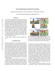
Figure 1: The proposed parameterizations In our experiments we have tested the linear method suggested by Gruen and the second order approximation of Levenberg-Marquardt. According to our experience the solution of the proposed optimization problem is very unstable if proper constraints are not used. The constraints we have chosen are of two di�erent nature. Geometric constraints identi ed by the epipolar geometry and physical constraints de ned by a set of common sense bounds imposed on the possible reciprocal orientation and position of the two cameras. Both constraints can be translated into bounds to the degrees of freedom of the template matching. In our problem the template corners can slide on the epipolar lines, or in their neighbourhood. Only three of the four corners of the template are su�cient to de ne an a�ne base in the image plane. The knowledge of the epipolar geometry can only be known up to some precision. In order to cater for the erroneous orientation and position of the computed epipolar lines we have tried di�erent parameterizations. Errors in the computation of the epipolar geometry can be taken into consideration by allowing the corners of the template to move inside a band bisected by the epipolar line. This added degree of freedom can be considered as a new parameter in the optimization functional. The band can be de ned either by one parameter, the same for the three bands, or by three parameters, a new one for each band. Figures 1(a),(b) and (c) show how the chosen parameterizations work. The �i are the new parameters which are functions of the a�ne parameters a. The optimization is performed on the �i and then the correspondent optimal a�ne parameters are derived. Experiments have been tested for the three di�erent parametrizations. In order to solve our constrained optimization problem we have chosen a well tested public domain software package. It is called CFSQP (an acronym which stands for C code for Feasible Sequential Quadratic Programming). Such optimization package is composed of a set of C functions for the minimization of the maximum of a set of smooth object functions. It handles linear and non-linear equality and inequality constraints and also bounds on the used variables. CFSQP turns all the non-linear equality constraints into linear inequalities and uses penalty functions to solve the problem. 13
3 EXPERIMENTAL RESULTS This section presents the experiments which were carried out to test the proposed approach. First of all we show that an a�ne transformation is a good approximation to the ideal homography which relates two projective views of a planar patch. Then we describe the used set-up. Finally we discuss all the experiments and we draw some conclusions.
3.1 A�ne approximation In order to prove that an a�ne transformation is a good approximation to the homography we describe a simple simulation experiment. We assume a simulation setup where a stereo rig is viewing a plane. The extrinsic and intrinsic parameters of the two cameras are supposed to be known together with the exact location of the plane and its orientation. Without any loss of generality we have chosen the position of one of the two cameras as the external reference frame and we have assumed both cameras identical. Under such ideal conditions if a point is selected from the rst image it is always possible to compute the corresponding point lying on the plane and then retrieve the exact location of its projection onto the second image plane. Let us call m1i and m2i the generic correspondence in the two image planes coordinates.
(a) Plane parallel to a virtual plane
(b) Plane in generic position
Figure 2: Error distribution obtained by comparison of exact mapping (homography) and approximating a�ne If K1 and K2 are the two intrinsic parameter matrices for the two views, we can write m1i = K1 � x1i m2i = K2 � x2i which transform the camera frame coordinates of a point, x1i for instance, into the corresponding image frame coordinates, in our example m1i . On the other hand, any two generic points expressed in the two camera frame coordinates can always be related by the following equation T x2i = (R + t nd ) � x1i where R and t represent respectively the rotation and translation between the two camera coordinate frames. Such formula can be easily derived by the knowledge of the plane parameters (n is its normal vector and d its distance to an external frame, in our speci c case the rst camera frame) and the two viewing plane relationships R and t. Combining the last two equations we obtain T m2i = K2 � (R + t nd ) � K1? � m1i which is the relation between the coordinates of a point lying on the rst image plane and the ones of its correspondent lying on the second image. From the knowledge of the correspondences of a set of points (a 9
1
template of the rst image) we can compute an approximate mapping. We used a standard least square method to estimate the approximating a�ne transformation parameters. At this stage it is possible to compare the exact correspondence with the approximated one. Results are shown in Figure 2. The two histograms illustrate the error distribution (euclidean distances measured in pixels between estimated and expected 2D position) in the case the transformation between the two views is identi ed by a translation t along the x (horizontal) axis of 0.1m and a simple rotation around the z (vertical) axis of 3 degrees (the simulation setup was chosen close to the real setup). The two histograms show two experiments. In the rst the viewed plane is parallel to the plane passing through the two centers of perspective and parallel to the z axis. In the second experiment the plane has a general orientation. As it can be noticed the errors are small even taking into consideration the tails of the distribution, the maximum error is less than 0.005 pixels. The derived results allow us to say that the a�ne transformation is a good approximation of the theoretic homography. In addition we can conclude that large errors in the minimization can only be introduced by the optimization routines.
3.2 The used setup
Figure 3: The used setup In order to test our method we have chosen to use a simple setup. A calibration grid was placed in ve positions at di�erent depths from the two cameras with a relatively slanted orientation (see Figure 3). The taken images had a peripheral distortion of 0.5 pixel, and all the experiments were performed far from the image border. Using a model based corner matching technique we have computed the epipolar geometry between the two views . We used 460 points to compute the epipolar geometry. The number of points has to be large to produce a stable epipolar geometry. 6
14
The goodness of the retrieved epipolar geometry is shown in Figures 4 and 5. The rst pictures (Figures 4(a) and 4(b)) represent a simple qualitative illustration of the result. They represent a point and the epipolar line where the point should lie. This point was used to compute the epipolar geometry. As it can be seen the epipolar geometry is very accurate (Figure 4(a)). In order to study the stability of the matching process we have produced a less accurate epipolar geometry by using only 20 points out of the existing 460. A qualitative illustration of this second epipolar geometry is shown in Figure 4(b). Figures 5(a) and 5(b) describe the histograms of the error distribution derived from the distance line-point.
(a) Accurate computation, 460 points
(b) Inaccurate computation, 20 points
Figure 4: Qualitative illustration of the computed accurate and inaccurate epipolar geometry. Each graph shows a zoom on a point and its corresponding epipolar line.
(a) Accurate epipolar geometry
(b) Inaccurate epipolar geometry
Figure 5: Epipolar line-point euclidean distance distribution (horizontal scale in pixel). The two distributions had to be di�erently scaled to better show their shape.
The two graphs illustrate both cases with accurate and less accurate epipolar geometry. A at picture (see Figure 3) was then placed in the third position (middle position) used during the weak calibration process. All the performed tests make use of 2627 points taken out of such picture. For a correct use of template matching it is indispensable to understand what is the optimal template size. In order to do so we have chosen to test our method with di�erent template sizes, namely 5x5, 11x11, 17x17 and 27x27. Such tests are a standard technique for template matching . The use of di�erent template sizes usually shows the fact that the larger the template the more information is hold inside the selected region and the more likely is the inclusion of a correct match. However there is a drawback, in fact the larger is the template size the more likely is the occurance of discontinuities and therefore the introduction of mismatches or even large errors. It is therefore important to nd a tradeo� between template size and performance. Tests were carried out using di�erent template sizes and the three di�erent parameterizations described in Section 2. In addition a simple 2-parameter optimization was used to show that when template deformation is not taken into account results are much worse. During the optimization process such parameterization takes into account the only translation of the undeformable template along or perpendicular to the epipolar line. 2
3.3 Matching veri cation Tmpl. size Parametriz. Mean Std. Dev. Med. Std. Med. Dev. % Out. Acc 2 param 4.71 6.02 2.05 3.05 13.97 3 param 1.43 3.24 0.30 0.44 14.27 4 param 1.51 2.97 0.40 0.60 14.92 5�5 6 param 1.51 2.91 0.38 0.56 15.45 Inacc 2 param 4.55 6.00 1.73 2.57 16.67 3 param 1.93 3.81 0.43 0.64 16.25 4 param 1.90 3.36 0.45 0.67 18.84 6 param 1.66 3.10 0.39 0.59 17.01 Acc 2 param 0.66 1.62 0.24 0.37 8.26 3 param 0.11 0.25 0.06 0.10 3.42 4 param 0.10 0.18 0.07 0.10 2.20 17 � 17 6 param 0.11 0.27 0.07 0.10 2.89 Inacc 2 param 0.74 1.96 0.24 0.36 8.94 3 param 0.15 0.27 0.08 0.12 7.00 4 param 0.10 0.20 0.07 0.10 1.94 6 param 0.14 0.32 0.08 0.12 3.08
Table 1: Quality alignment In order to analyse the results we followed two di�erent ways. We rst of all tried to verify the alignment constraint. From a result of projective geometry aligned points undergoing a projective transformation remain
aligned if a homographic transformation is applied to the projective plane. In order to make use of such result we used a couple of views of the at picture (see Figure 3). In the rst image we selected aligned 2D projections of 3D coplanar points. The expected collinearity of the correspondent 2D points in the second image was used to test our matching technique. Statistics were computed by tting a line to the second image points (following a least median square technique ) and computing the euclidean distance between supporting points and such line. 17
Table 1 illustrates the statistics related to the line-point distances. The table summarizes the statistics (mean, standard deviation, median, standard median deviation and percentage of outliers) for the cases of accurate and less accurate epipolar geometry. Experiments were carried out for di�erent template sizes. The table illustrates only the case of a small template (5 � 5) and what we selected as optimal template size (17 � 17). The median was preferred to the mean because of the existence of outliers. The standard median deviation (we used the formula � = 1:4826 � (1+5:0=(nb ? 4:0)) � med where nb is the used number of points and med is the median) was chosen to
16
estimate robustly the accuracy of the results and to compute the percentage of outliers. A closer look at the table shows that the accuracy is clearly better when the larger template (17 � 17) is used, and this even independently of the type of used epipolar geometry. Besides an accurate epipolar geometry always gives better results than a less accurate one, a part from the two-parameter optimization. As expected the two-parameter optimization does not o�er acceptable results. In a second stage we have computed an accurate approximation of the homography which maps the rst view of a planar object onto the second. A least square technique was then used to estimate the approximation of the homographic mapping. Such mapping was then used to verify the match produced by the optimization technique. The euclidean distance between the accurate match and the estimated one was used to measure the accuracy of our optimization technique. Histograms and tables are used to show their distribution and the related statistics. Tmpl. size Parametriz. Mean Std. Dev. Med. Std. Med. Dev. % Out. Acc 2 param 5.46 6.52 2.12 3.15 15.98 3 param 1.49 3.14 0.39 0.59 12.48 4 param 2.01 2.97 0.88 1.30 11.07 5�5 6 param 1.97 2.79 0.91 1.36 11.18 Inacc 2 param 5.29 6.36 2.01 3.00 16.70 3 param 2.33 3.65 1.06 1.58 12.10 4 param 2.42 3.36 0.96 1.43 14.26 6 param 2.14 3.01 0.96 1.43 12.59 Acc 2 param 1.97 3.87 0.75 1.12 10.46 3 param 0.33 0.50 0.24 0.36 1.94 4 param 0.68 1.17 0.42 0.62 3.72 11 � 11 6 param 0.67 0.85 0.44 0.66 3.19 Inacc 2 param 1.80 3.50 0.75 1.11 9.55 3 param 0.88 0.82 0.78 1.16 0.60 4 param 0.68 1.19 0.41 0.62 3.91 6 param 0.62 0.58 0.44 0.66 2.28 Acc 2 param 1.06 1.67 0.70 1.04 3.34 3 param 0.27 0.26 0.23 0.34 0.57 4 param 0.39 0.24 0.34 0.51 0.30 17 � 17 6 param 0.29 0.27 0.27 0.40 0.72 Inacc 2 param 1.15 2.02 0.70 1.05 3.91 3 param 0.78 0.50 0.73 1.08 0.00 4 param 0.38 0.25 0.34 0.51 0.34 6 param 0.42 0.38 0.35 0.52 1.10 Acc 2 param 1.03 0.83 0.92 1.37 0.57 3 param 0.25 0.08 0.24 0.36 0.00 4 param 0.27 0.10 0.26 0.39 0.00 27 � 27 6 param 0.28 0.11 0.27 0.41 0.00 Inacc 2 param 1.05 0.78 0.97 1.45 0.39 3 param 0.76 0.45 0.71 1.06 0.00 4 param 0.28 0.10 0.27 0.41 0.00 6 param 0.28 0.11 0.27 0.41 0.00
Table 2: Positioning quality measured in pixel Table 2 illustrates the results for a large number of experiments. Experiments with the four mentioned parameterizations were carried out. The same statistics presented in Table 1 are used to illustrate the accuracy of the results. The table shows results for four di�erent template sizes. A comparison of the standard median deviations shows that the larger the template the better are the results, independently of the accuracy of the epipolar geometry. The two-parameter optimization results the only anomaly and it shows that such parameterization is unreliable to obtain subpixel accuracy. If each template size is separately analysed it can be noticed that an
(a) Accurate 3 parameters
(b) Inaccurate 3 parameters
(c) Accurate 4 parameters
(d) Inaccurate 4 parameters
(e) Accurate 6 parameters
(f) Inaccurate 6 parameters
Figure 6: Line-point euclidean distribution for the 3 presented parameterizations. All graphs a part from histogram (b) are normalized and have the same scale
accurate geometry always gives better results. Even if the largest template (27 � 27) o�ers the best results we have chosen the 17 � 17 template size because of its average size. E�ciency is the main reason: for the larger the template the slower results the optimization process. We also publish six histograms (Figures 6) which illustrate the density function for the cases of a 17x17 size template with accurate and less accurate epipolar geometry and for the three di�erent techniques (3, 4 and 6 parameters). The histograms for the three-parameter optimization shows a particular phenomenon which must be taken into consideration for a correct analysis of the results. Such parameterization allows the movement of the template during the optimization process only along the epipolar lines. An error along the direction perpendicular to an epipolar line would be weighted the same for both small and large distances introducing a non-negligible bias in the results. In the case of accurate epipolar geometry the bias is reduced. This can be noticed in histograms 6(a) and 6(b). The horizontal scale has been changed for the inaccurate case to show the greater data spread introduced by the inaccuracy of the epipolar geometry. Histograms 6(c) and 6(d) show that such bias is reduced in the case of a four-parameter optimization. The best results are produced by the six-parameter technique. Histograms 6(e) and 6(f) show such results.
4 CONCLUSIONS AND FUTURE WORK The paper has studied a technique which allows the identi cation of similar image patches from two consecutive views taken with weakly calibrated cameras. The comparison of two consecutive views selected from a sequence is the rst step towards the achievement of a three-dimensional reconstruction of the scene. The ner is the accuracy of the matches, the more accurate is the obtained reconstruction. The proposed technique uses an adaptive template matching. It works as an iterative optimization of the involved parameters with a consequent iterative re nement of the correspondence. Matching is performed by transforming a template window using the current image-to-image a�ne transformation and exploiting the epipolar geometry to reduce the degrees of freedom of the template position in the region of interest. We showed that subpixel accuracy can be reached with relatively small templates (17 � 17). In the case of a stereo pair undergone an estimated distortion of 0.5 pixel (10 �m of pixel size) it is shown an accuracy between 3 and 5 �m for template windows of 17x17 size selected in textured image patches. The current implementation was a simple testbed to demonstrate that a very good accuracy can be reached using an adaptive template matching. We are currently studying how to improve the accuracy and speed up the process. Some parallel research in our group has shown very interesting results obtained by implementing robust statistics techniques in the matching stage of the optimization process to be able to match points even when occlusions occur. We envisage to fully integrate such technique in the body of our optimization process. Our future plan also includes a technique able to reconstruct a 3D model of the scene by means of an incremental construction based on the found matches.
ACKNOLWEDGEMENTS We would like to thank the authors of the public domain software package CFSQP, the use of their software turned out precious in the testing stage of our technique. We also would like to thank Dr Long Quan and Zhong-Dan Lan for their useful input.
5 REFERENCES [1] J. Aloimonos, I. Weiss, and A. Bandyopadhay. Active vision. International Journal of Computer Vision, pages 333{356, 1988. [2] P. Aschwanden and W. Guggenbuhl. Experimental results from a comparative study on correlation-type registration algorithms. In Forstner and Ruwiedel, editors, Robust Computer Vision, pages 268{282. Wichmann, 1992. [3] R. Bajcsy. Active perception. Proceedings of the IEEE, 76(8):996{1005, August 1988. [4] R. Bajcsy and M. Campos. Active and exploratory perception. Computer Vision, Graphics and Image Processing: Image Understanding, 56(1):31{40, July 1992. [5] E.P. Baltsavias. Multiphoto Geometrically Constrained Matching. PhD thesis, ETH-Zurich, 1992. [6] P. Brand and R. Mohr. Accuracy in image measure. In Videometrics III, SPIE's 1994 international symposium on photonic sensors & controls for commercial applications, October 1994. to appear. [7] F. Devernay and O.D. Faugeras. Computing di�erential properties of 3-D shapes from stereoscopic images without 3-D models. In Proceedings of the Conference on Computer Vision and Pattern Recognition, Seattle, Washington, USA. IEEE Computer Society Press, June 1994. [8] U.R. Dhond and J.K. Aggarwal. Structure from stereo { a review. Ieee Transactions on Systems, Man, and Cybernetics, 19(6):1489{1510, November 1989. [9] O. Faugeras. Three-Dimensional Computer Vision - A Geometric Viewpoint. Arti cial intelligence. M.I.T. Press, Cambridge, MA, 1993. [10] R. Fletcher. Practical Methods of Optimization. John Wiley and Sons, second edition, 1987. [11] P. Gill, W. Murray, and M. H. Wright. Practical Optimization. Harcourt Brace Jovanovich, Publishers, 1989. [12] A.W. Gruen. Adaptative least squares correlation: a powerful image matching technique. S. Afr. Journal of Photogrammetry, Remote Sensing and Cartography, 14(3):175{187, 1985. [13] C.T. Lawrence, J.L. Zhou, and A.L. Tits. User's Guide for CFSQP Version 2.0. Technical Report tr-94-16, University of Maryland, University of Maryland, MD, February 1994. [14] Q.T. Luong. Matrice Fondamentale et Autocalibration en Vision par Ordinateur. Th�ese de doctorat, Universit�e de Paris-Sud, Orsay, France, December 1992. [15] Q.T. Luong, R. Deriche, O.D. Faugeras, and T. Papadopoulo. On Determining the Fundamental Matrix. Technical Report 1894, INRIA, Sophia-Antipolis, France, 1993. [16] P. Meer, D. Mintz, A. Rosenfeld, and D.Y. Kim. Robust regression methods for computer vision: a review. International Journal of Computer Vision, 6(1):59{70, 1991. [17] D. Mintz and P. Meer. Robust estimators in computer vision: an introduction to least median of squares regression. In Y.A. Feldman and A. Bruckstein, editors, Arti cial intelligence and computer vision, pages 61{70. Elsevier Science, 1991. [18] W.K. Pratt. Digital Image Processing. Wiley-Interscience, 1978. [19] W.H. Press, B.P. Flannery, S.A. Teukolsky, and W.T. Vetterling W.T. Numerical Recipes in C. Cambridge University Press, 1988. [20] M. Sonka, V. Hlavac, and R. Boyle. Image Processing, Analysis and Machine Vision. Chapman and Hall, 1993.