Cost-Based Query Optimization for Complex Pattern Mining on Multiple Databases Ruoming Jin
Dave Fuhry
Abdulkareem Alali
Department of Computer Science Kent State University Kent, OH, 44242
Department of Computer Science Kent State University Kent, OH, 44242
Department of Computer Science Kent State University Kent, OH, 44242
[email protected]
[email protected]
ABSTRACT For complex data mining queries, query optimization issues arise, similar to those for the traditional database queries. However, few works have applied the cost-based query optimization, which is the key technique in optimizing traditional database queries, on complex mining queries. In this work, we develop a cost-based query optimization framework to an important collection of data mining queries, i.e. frequent pattern mining across multiple databases. Specifically, we make the following contributions: 1) We present a rich class of queries on mining frequent itemsets across multiple datasets supported by a SQL-based mechanism. 2) We present an approach to enumerate all possible query plans for the mining queries, and develop a dynamic programming approach and a branch-and-bound approach based on the enumeration algorithm to find optimal query plans with the least mining cost. 3) We introduce models to estimate the cost of individual mining operators. 4) We evaluate our query optimization techniques on both real and synthetic datasets and show significant performance improvements.
1. INTRODUCTION Over the last several years, data mining algorithms and tools have become increasingly important for data analysis and decision making processes. Some of the standard data mining algorithms, including association rule mining and various clustering and classification tools, have been incorporated into major commercial DBMSs, such as Oracle 10g [21], IBM DB2 [35], and SQL Server 9.0 [31]. However, data mining is an interactive and iterative process. A data miner cannot expect to get the desired results or knowledge by a single execution of the data mining operators. Especially, the data mining query can become rather complicated as the data miner has to compare and extract patterns from multiple correlated data sources and/or put various constraints on the data mining operators. To evaluate a complex data mining query efficiently, the database system is very likely to invoke data mining operators several times [18]. The selection of mining operators and the order in which they are
Permission to make digital or hard copies of all or part of this work for personal or classroom use is granted without fee provided that copies are not made or distributed for profit or commercial advantage and that copies bear this notice and the full citation on the first page. To copy otherwise, to republish, to post on servers or to redistribute to lists, requires prior specific permission and/or a fee. EDBT’08, March 25–30, 2008, Nantes, France. Copyright 2008 ACM 978-1-59593-926-5/08/0003 ...$5.00.
[email protected]
invoked can significantly affect the mining cost. Therefore, the query optimization problem, i.e., how to find the query plan with the optimal cost, is becoming an important issue to speed up the mining process for complex mining queries. In the traditional database systems, the cost-based optimization technique has proven to be one of the keys for handling the query optimization [5]. A natural question to ask is “will such cost-based optimization be applicable to complex data mining queries?” However, there are only a few works which address this very important question and there are many challenges in answering this question. For instance, the cost of the mining operators is very hard to estimate as their procedures are not only much more complicated than standard relational operators, but also their costs are dependent on the properties of the data being processed. In addition, to formally define all the valid query plans for a mining query and then efficiently identify the optimal one is not straightforward. In this paper, we address the cost-based query optimization problem for data mining queries. We target an important class of frequent pattern mining tasks involving the discovery of interesting patterns from multiple, distinct datasets (Listed as the Q1-type query in Section 2). For example, a manager of a nation-wide store would like to know what itemsets are frequent in stores in New York and New Jersey, but very infrequent in stores in California. Similarly, biology researchers are interested in protein primary sequences that appear frequently in the human genome but infrequently in the chicken genome, and/or, the sequences that appear frequently in both species. Such complex mining queries give rise to the aforementioned mining query optimization problem as follows. Suppose a user needs to find itemsets that are frequent with a certain support in both A and B. While this can be answered by taking the intersection of the results from both A and B, this is likely to be very expensive. Instead, we can compute itemsets frequent in either of the two datasets, and then simply find which of these are frequent in the other dataset. However, this leads to two different evaluation plans, corresponding to using either dataset A or dataset B for the initial evaluation. The two evaluation plans can have different costs, depending upon the nature of the datasets A and B. Furthermore, as the number of datasets and the complexity of the query condition increases, the number of possible evaluation plans can also grow. In [18], due to the complexity of mining operators and mining queries, all the query optimization is performed based on greedy heuristics. In this paper, we present the first cost-based query optimization framework for these types of complex mining queries across multiple databases. We address a list of open problems for cost-based mining query optimization, including 1) how to system-
Dataset A1 TransID Items 1 {1, 2, 5} 2 {2, 4} 3 {1, 2, 5} 4 {1, 3, 4 } 5 {2, 3, 4} 6 {1, 3,4} 7 {1, 2 } 8 {1, 2, 3, 4, 5 }
Dataset A2 TransID Items 1 {1, 2, 4, 5} 2 {2, 3, 5} 3 {1, 2, 5 } 4 {1, 2, 3} 5 {1, 3 } 6 {3, 4}
Table 1: Datasets A1 and A2 atically enumerate possible query plans, 2) how to estimate the cost of different mining operators, and finally 3) how to find a query plan with the least mining cost. Specifically, we make the following contributions: 1. We present a richer class of frequent itemset queries across multiple datasets supported by a SQL-based mechanism, which is much beyond [18] (Section 2). 2. We present an approach to enumerate all possible query plans for the mining queries (Section 4). 3. We present a dynamic programming approach and a branchand-bound approach to find optimal query plans with the least mining cost (SubSection 5). 4. We introduce models to estimate the cost of individual mining operators. (SubSection 5.1 and 5.2) 5. We evaluate our query optimization techniques on both real and synthetic datasets (Section 6) and show significant speedup compared with the heuristic approaches.
2. SQL EXTENSIONS FOR MINING ACROSS MULTIPLE DATASETS In this section, we introduce a rich class of queries based on a SQL based mechanism for querying frequent itemsets across multiple datasets. Note such queries mainly serve for exploration purposes of mining task optimization. Let {A1 , A2 , · · · , Am } be the set of datasets we are targeting. Each of these comprises of transactions, which are sets of items. The datasets are also homogeneous, i.e, an item has an identical name across different datasets. Let Itemi be the set of items for the dataset Ai . For a dataset Ai , we define the following table, SofAi(I, Supp) Where the first column stores all possible itemsets in the dataset Ai, and the second column stores the support of the itemsets in the dataset. We refer to the table SofAi as a support table. Clearly, the support table can only be used as a virtual table or a logical view, as the total number of itemsets is likely to be too large for the table SofAi to be materialized and stored. We further define two views based on the individual support tables to facilitate the mining queries on multiple datasets. The first view is referred to as F table, and is defined as follows. CREATE VIEW F(I, SuppA1, ..., SuppAm) AS ( SELECT (CASE WHEN SofA1.I is not null THEN SofA1.I ... WHEN SofAm.I is not null
I {1} {2} {3} {4} {5} {1, 2} {1, 3} : {1, 2, 3, 4, 5}
A1 6/8 6/8 4/8 6/8 3/8 4/8 3/8 : 1/8
A2 4/6 4/6 4/6 2/6 3/6 3/6 2/6 : 0
Table 2: F Table for the Datasets A1 and A2 Dbid 1 1 1 1 1 1 : 1 2 2 2 : 2
I {1} {2} {3} {4} {5} {1, 2} : {1, 2, 3, 4, 5} {1} {2} {3} : {1, 2, 3, 4, 5}
Supp 6/8 6/8 4/8 6/8 3/8 4/8 : 1/8 4/6 4/6 4/6 : 0
Table 3: S Table for the Datasets A1 and A2 THEN SofAm.I) AS I SofA1.Supp AS SuppA1, ... SofAm.Supp AS SuppAm FROM SofA1 FULL OUTER JOIN SofA2 ON SofA1.I=SofA2.I FULL OUTER JOIN SofA3 ON SofA2.I=SofA3.I ... FULL OUTER JOIN SofAm ON SofAm-1.I=SofAm.I )
Note that the first column, F.I, stores all the possible itemsets in the m datasets. The second view, referred to as the S table is the dual representation of the F table, which are simply the union of the individual support tables as follows. CREATE VIEW S(Dbid, I, Supp) AS ( (SELECT 1, I, Supp FROM SofA1) UNION (SELECT 2, I, Supp FROM SofA2) UNION ... (SELECT m, I, Supp FROM SofAm) )
For example, consider two transaction datasets A1 and A2 , as shown in Table 1. The set of distinct items in the two datasets, Item, is {1, 2, 3, 4, 5}. Table 2 and 3 contain a portion of the F table and S table for the datasets A1 and A2 , respectively. In our SQL extensions, a frequent itemset mining task on multiple datasets is expressed as a SQL query to partially materialize the two virtual tables, F table and S table. In the following, we describe the different types of mining queries. To facilitate our discussion, we consider we have four datasets, A, B, C, and D. Our F table, and S table are defined according to our above discussion. For example, the F table is as follows. F(I, SupA, SuppB, SuppC, SuppD)
Query Q1. Simple Comparisons: The following query Q1 is an example. Q1: SELECT I, SuppA, SuppB, SuppC, SuppD FROM F WHERE (SuppA >= 0.1 AND SuppB >= 0.1 AND SuppD >= 0.05) OR (SuppC >= 0.1 AND SuppD >= 0.1 AND (SuppA >= 0.05 OR SuppB >= 0.05))
Here, we want to find the itemsets that are either frequent with support level 0.1 in both A and B, and frequent in D with support level 0.05, or frequent (with support level 0.1) in both C and D, and also frequent in either A or B (with support level 0.05). Note that this is the type of query we mainly focus on in [18]. In the following, we will illustrate some more complicated queries using the F and S tables. Query Q2. Group-by Queries: Group-by queries ask for the itemsets that are (in)frequent in a certain number of datasets. For example, the following query asks to find the itemsets that frequent with support level 0.1 in at least 3 out 4 datasets. Q2: SELECT Dbid, I, Supp FROM S WHERE Supp >= 0.1 GROUP BY I HAVING COUNT(*) >= 3
Note that such queries can be expressed on the F table, but in a more complicated format. Q2’: SELECT I, SuppA, SuppB, SuppC, SuppD FROM F WHERE (SuppA >= 0.1 AND SuppB >= 0.1 AND SuppC >= 0.1) OR ... OR (SuppB >= 0.1 AND SuppC >= 0.1 AND SuppD >= 0.1)
Q3. Queries on Union of Datasets: In such queries, the queries involve the datasets which are the union of individual existing datasets. The following query Q3 tries to find the itemsets that are frequent with support level 0.2 on dataset A union B, and B union C, but infrequent with support level 0.1 on dataset B. Q3: SELECT I, ds(SuppA,SuppB), ds(SuppB,SuppC), SuppB FROM F WHERE ds(SuppA,SuppB) >= 0.2 AND ds(SuppB,SuppC) >= 0.2 AND SuppB= 0.1 AND INCREASING(SuppA,SuppB,SuppC,SuppD)
Where, INCREASING(s1 , · · · , sn ) (or DECREASING) determines if the support s1 , · · · , sn are increasing (or decreasing).
Many other types of queries can be expressed using the above views. For example, the queries on association rules derived from different datasets can be expressed based on these views. Further, if we have tables of attributes for each item, we can ask queries on the properties of itemsets. In other words, we can perform constraint itemsets mining across multiple datasets. Due to space limitations, we do not describe the specifics of these operations in the paper. Finally, in order to simplify our discussion, we will focus on frequent itemset mining tasks. The key ideas in extending our work to other frequent patterns or structures, such as sequences, subtrees, and subgraphs, are presented in [17].
3.
ALGEBRA AND QUERY EVALUATION
In this section, we first review the algebra for expressing the information required to answer such a mining query and briefly discuss how a mining query in its SQL format can be mapped to an algebra expression (Subsection 3.1). Then, we introduce basic tools for reducing the query evaluation cost (Subsection 3.2). Finally, we describe a general representation, the M -table, for describing the all possible query plans (Subsection 3.3).
3.1
Basic Algebra for Queries
Our algebra contains only one mining operator SF and two operations, intersection (u) and union (t). Formally, they are as follows: The frequent itemset mining operator SF (Aj , α) returns a twocolumn table, where the first column contains itemsets in Aj which have the support level α, and the second column contains their corresponding frequency in the dataset dataset Aj . Intersection (F1 u F2 ): Let F1 and F2 be two tables whose first column contains a collection of itemsets, and other columns contain the corresponding frequency (possibly empty) in different datasets. The intersection operation (F1 u F2 ) returns a table whose first column contains the itemsets appearing in the first columns of both F1 and F2 , and other columns contain frequency information for these itemsets in the datasets appearing in F1 and F2 . Union (F1 t F2 ): The union operation (F1 t F2 ) returns a table whose first column contains the itemsets appearing in the first columns of either F1 or F2 , and other columns contain the frequency of these itemsets in the datasets appearing in F1 or F2 . Given this, we can directly model a restricted class of queries (a subset of Q1-type queries – simple comparison queries in Section 2) using the above operator and operations. This class of queries involves constraint conditions (the WHERE clauses) which do not contain any negative predicates, i.e., a condition which states that support in a certain dataset is below a specified threshold. We call this class of queries positive queries. Let us consider a positive query Q with the condition C. Clearly, the condition C can be restated in the DNF form, with conjunctive clauses C1 , . . . , Ck . Formally, C = C1 ∨ . . . ∨ Ck , Ci = pi1 ∧ . . . ∧ pim , 1 ≤ i ≤ k
where, pij = SuppAij ≥ α is a positive predicate, i.e., a condition which states that support in a certain dataset (Aij ) is greater than or equal to a specified threshold (α). The corresponding basic algebra expression is as follows. We replace pij by the operator SF (Aij , α). We can represent the query by F Q = F C1 t · · · t F Ck
where, in each FCi , the corresponding SF operator is connected using intersection operations. Therefore, for query Q1 , its corre-
sponding basic algebra expression FQ1 is as follows. A B C D
(SF (A, 0.1) u SF (B, 0.1)) u SF (D, 0.05) ⇒ F1 t(SF (A, 0.05) u SF (C, 0.1) u SF (D, 0.1)) ⇒ F2 t(SF (B, 0.0.5) u SF (C, 0.1) u SF (D, 0.1)) ⇒ F3
In [18], we have shown how a more general class of mining queries, which could involve negative conditions, can be expressed by this algebra as well. Essentially, the positive and negative queries capture the Q1 type queries, which involve only simple comparisons. More complicated queries, such as Q2 (Group-by), Q3 (Union), and Q4 (Trend) type queries, can be transformed into Q1-type queries with some additional constraints. The detailed transformation is beyond the scope of this paper. Since the optimization techniques for Q1-type queries can be applied to other queries, we make Q1-type optimizations the focus of the rest of this paper.
3.2 Basic Tools for Query Optimization Let us consider the naive evaluation of the basic algebra expression FQ1 for the query Q1 stated in the previous subsection. We need to invoke the SF operator 7 times, including mining frequent itemsets on datasets A, B, and D with two different supports 0.1 and 0.05, and on dataset C with support 0.1. To reduce the mining costs, we introduce the following basic tools. Frequent itemset mining operator with constraints CF (Aj , α, X) finds the itemsets that are frequent in the dataset Aj with support α and also appear in the set X. X is a set of itemsets that satisfies the down-closure property, i.e., if an itemset is frequent, then all its subsets are also frequent. This operator also reports the frequency of these itemsets in Aj . Formally, CF (Aj , α, X) computes the following view of the F table: X u SF (Aj , α)
The typical scenario where this operator helps remove unnecessary computation is as follows. Suppose the frequent itemset operator intersects with some view of the F table, such that the projection of this view on the attribute I is X. This operator pushes the set X into the frequent itemset generation procedure, i.e., X serves as the search space for the frequent itemset generation. Containing Relation: The containing relation is as follows: β ≤ α, SF (Aj , β) contains all the frequent itemsets in SF (Aj , α). Therefore, if the first one is available, invocation of the second can be avoided. Instead, a relatively inexpensive selection operator, denoted as σ, can be applied. Formally, for β ≤ α, we have, SF (Aj , α) = σAj ≥α (SF (Aj , β))
This containing relations can be also extended to the the new CF mining operator. We note that another mining operator GF has been introduced in [18]. Given a number of datasets, it finds the itemsets that are frequent in each individual dataset with user-specified support levels. Our previous study [18] has shown a systematic way to incorporate the GF mining operator in the mining process, and is based on the optimal query plans generated from the SF and CF mining operators. To simplify our discussion, we will focus on finding optimal query plans using the SF and CF mining operators in this paper. In the next subsection, we will introduce an intuitive method which can help us to describe and generate possible query plans.
3.3
M -table:
A Unified Query Evaluation Scheme
D EFINITION 1. Assume the basic algebra expression of a query Q is FQ = F 1 t · · · t F t
F1 0.1 0.1 0.05
F2 0.05 0.1 0.1
F3 0.05 0.1 0.1
Table 4: M-table for the query Q1 F1 F2 F3 F4 F5 A 0.1 0.1 0.05 B 0.1 0.1 0.05 C 0 0 0.1 0.1 0.1 D 0.05 0.1 0.1 0.1 Table 5: An Uncolored M-Table where, each Fi involves intersection among one or more SF operators. Let m be the number of distinct datasets that appear in F . Then, the M -table for the basic algebra expression of this query is a table with m rows and t columns, where the row i corresponds to the dataset Ai , and the column j corresponds to the clause Fj . If SF (Ai , α) appears in Fj , the cell at the j-th column and i-th row will have α, i.e., Mi,j = α. Otherwise, the cell Mi,j is empty. As an example, the M table for the query Q1 in Section 2, has 4 rows and 3 columns and is shown in Table 4. Now, we focus on query plan generation using the M -table and the operators we have defined so far. To facilitate our discussion, we will use the M table in Table 5 as our running example. One of the most important features of M table is that it can capture the evaluation process for a query by using a simple coloring scheme. Initially, all the cells are non-colored (white). The operators, SF and CF , can color a number of non-empty cells black (shaded). The query evaluation process is complete when all non-empty cells are colored black. As a running example, consider applying SF (A, 0.05), SF (C, 0.1), CF (B, 0.1,SF I (A, 0.1)), and CF (D, 0.1,SF I (C, 0.1)) consecutively on an initially non-colored M -table (Table 5), where SF I is the projection of SF results on the itemset column. Table 6 shows the resulting partially colored table. We now define how each operator colors the table. Frequent itemset mining operator SF (Ai , α): An invocation of the frequent mining operator on the dataset Ai , with support α, will turn each non-empty cell at row i which is greater than or equal to α black. In our example, the first operator, SF (A, 0.05), will turn the cells M1,1 , M1,2 , and M1,4 black. The second operator, SF (C, 0.1), will turn the cells M3,3 , M3,4 , and M3,5 black. Frequent itemset mining operator with constraint CF (Ai , α, X): The coloring impacted by this operator is dependent on the current coloring of the table M . Let X be the set of frequent itemsets defined by all the black cells, and let S be the set of columns where these black cells appear. Then, by applying this operator on dataset Ai with support α, all cells on row i whose column is in the set S, and whose value is greater than or equal to α, will turn black. In our running example, the third operator CF (B, 0.1, SF I (A, 0.1))
A B C D
F1
F2
0.1 0.1 0
0.1 0.1 0 0.05
F3
F4
F5
0.05 0.1 0.1
0.1 0.1
0.05 0.1 0.1
Table 6: The Partially Colored M-Table
picks the black cells M1,1 and M1,2 by the parameter X = SF I (A, 0.1)
The set S includes the first two columns. Therefore, this operator turns the cells M2,1 and M2,2 black. Similarly, the fourth operator turns the cells M4,3 , M4,4 , and M4,5 black. By the above formulation, the query evaluation problem has been converted into the problem of coloring the table M . The possible query plans can be intuitively captured in this framework. Note that different operators can be used, and in different order, to color the entire table black. There are different costs associated with each of them. In the rest of the paper, we will develop cost-based query optimization approaches to find optimal query plans for our mining queries. In Section 4, we will describe an approach based on the M -table to systematically traverse the space of query plans. In Section 5, we will introduce two cost-based methods to find optimal query plans and discuss the cost estimation for different mining operators. In Section 6, we will evaluate the efficiency of our query optimization techniques on both real and synthetic datasets.
4. QUERY PLAN ENUMERATION In this section, we will first define the search space of all possible query plans for our mining queries (Subsection 4.1). Then, we will discuss how to identify equivalent query plans, and how to avoid generating duplicate query plans (Subsection 4.2). Further, we introduce several heuristics to reduce the search space of query plans (Subsection 4.3). Finally, the detailed enumeration algorithm is described (Subsection 4.4). Note that the query enumeration approach developed in this section will be the basis of our optimal query plan generation, which will be discussed in Section 5.
4.1 Query Plan Space As discussed in the last section, each mining operator will color a group of cells in the same row of the M -table, MQ , and a query plan will color all the nonempty cells in MQ . Therefore, query plan enumeration can be transformed to list all possible ways to color the M -table. To facilitate our discussion, we denote a group of cells in the same row of the M -table as a cell-set. Formally, a sequence of cell-sets, i.e. < s1 , s2 , · · · , sm >, where si is a cellset and the union of all cell-sets covers all the nonempty cells in the M -table, can be used to represent query plans. Next, we will apply the following two steps to uniquely map a sequence of cellsets which colors all the nonempty cells in the M -table to a single query plan. Step 1: In the first step, we will split a sequence of cell-sets into two phases. The first phase (Phase 1) contains only the SF operators, and the second phase (Phase 2) contains the CF mining operators. This is equivalent to dividing a query plan into two phases. Note that such a two-phase query plan schema can help us uniquely map a cell-set in the first phase to a single SF mining operator. Finally, we point out that the reason we can schedule SF mining operators before CF mining operators is because the invocation of SF operators is always independent of the mining results generated from any other mining operators in a query plan. Step 2: In order to map a cell-set in the second phase to a CF mining operator, i.e. CF (Aj , α, X), we need to provide the set X which constrains the search space of itemsets. The fewer itemsets CF will have to traverse, the less CF will cost. Thus, we will always choose the CF operator with the maximal constraints X, which corresponds to the smallest search space needed to color a cell-set in a query plan. For example, considering in Table 6, we
need to map the cell-set containing the first two cells in the third column, M3,1 and M3,2 , to a CF mining operator. We assume SF (A, 0.1) and SF (B, 0.1) are used to color the cells in the first row and second row respectively. In this case, we will choose X to be SF I (A, 01) ∩ SF I (B, 01), instead of only SF I (A, 0.1) or SF I (B, 0.1) for the corresponding CF mining operator. This is because our choice X uses all the available constraints, defined in terms of the first two cells in both the first and second rows. Given this, we can see that a sequence of cell-sets can uniquely determine a single query plan. However, we note that different sequences of cell-sets may correspond to essentially the same query plan. This problem is critical to query plan enumeration because we need to avoid generating duplicate query plans. We are going to address this issue in the next subsection.
4.2
Partial Orders and Equivalent Query Plans
The reason that two query plans, described as two sequences of mining operators, or correspondingly, cell-sets, are equivalent is because the invocation orders of some mining operators can be changed. For example, consider the following query plan QP 0 to color the M table in Table 5. P hase1 :
SF (A, 0.1), SF (C, 0.1);
P hase2 :
CF (B, 0.1, SF I (A, 0.1)); CF (D, 0.1, SF I (C, 0.1)); I
CF (A, 0.05, SF (C, 0.1) ∩ SF I (D, 0.1)); CF (B, 0.05, SF I (C, 0.1) ∩ SF I (D, 0.1)); CF (D, 0.05, SF I (A, 0.1) ∩ SF I (B, 0.1)); CF (C, 0, SF I (A, 0.1) ∩ SF I (B, 0.1));
In this example, we can clearly switch the invocation order of the first two mining operators in phase 2 with the same mining cost. However, the second and the third CF mining operators can not be exchanged since the later one relies on the first one’s mining results. To recognize the equivalent query plans systematically, we introduce the following formal definitions for query equivalence. Two query plans are equivalent if their phase 1 and phase 2 are both equivalent. The phase-1 equivalence is fairly straightforward since the SF mining operators can be invoked in any order. D EFINITION 2. Two query plans are phase-1 equivalent if they share the same set of SF mining operators. The phase-2 equivalence will be defined in terms of a partial order defined on CF mining operators. We will begin with the following simple relationship ( s]pi logpi
i=1
where N is the total number of distinct items in the dataset, fi is frequency of itemsets, pi is the probability of observing 2-itemset i in the dataset, and s is the support level. If the 2-itemset i is frequent, i.e. fi > s, the truth function [fi > s] returns 1, otherwise, it returns 0. All of the four factors can be calculated or maintained for each dataset. In order to provide a reasonable estimate of SF mining 1
This is slightly different from the original paper, where the truth function is [pi > s]. After communicating with the authors, the above formula is confirmed to be correct one.
operator cost, we first collected the running time C of SF mining operations on a collection of real and synthetic datasets with different support levels. Then, utilizing linear regression analysis, we found that for a given dataset, a good linear regression model for the running time of SF operator is given by log C = β0 + β1 s + β2 d This basically suggests that the mining cost (specifically, running time C) is exponentially correlated with support s and density d. However, though this type of linear model provides good estimation results, it requires parameter fitting for each individual dataset, i.e. the β parameters vary from dataset to dataset. This can be too computationally expensive to use in a database-like mining system. Given this, we then try to establish a more generalized linear prediction model using the characteristics of each individual dataset, including number of transactions n and the average of length of transactions |I| for a dataset. Choosing from a list of probable models and using linear regression analysis, we found the following model log C = β0 + β1 s + β2 d + β3 log n + β4 log |I| provides the best prediction accuracy for the mining cost of SF . Therefore, we apply this model with the parameters computed from the regression analysis to predict the SF mining cost. In addition, we note that density d is query dependent, i.e., its value depends on support s. To compute d online for a given query can be too costly. Instead, we pre-compute d for a given dataset by an average of d over a sample of supports s. Cost Estimation for CF : Similar to SF , the CF mining operator can be realized in different ways. Our current implementation is based on the implementation of the SF mining operator. Specifically, for CF (Aj , α, X), the set of itemsets X is initially put into a hash table. Then the processing of CF is similar to the frequent itemset mining operator, with one exception in the candidate generation stage. While placing an itemset in the candidate set, not only do all its subsets need to be frequent, but the itemset needs to be in the hash table as well. Considering the cost of CF mining operator to be very dependent on the size of the search space provided in the input parameter X, we will estimate the cost of CF (A, α, X) as follows. C(CF (A, α, X)) = C(SF (A, α)) ×
|SF I (A, α) ∩ X| |SF I (A, α)|
(1)
where C(CF) and C(SF) represent the cost of the CF and SF mining operators, respectively. I (A,α)∩X| A possible way to estimate |SF without actually in|SF I (A,α)| voking the SF and CF mining operators is to utilize the 1-itemsets or 2-itemsets to represent all the frequent itemsets in dataset A and X. This requires us to either pre-compute all the 1-itemsets and/or 2 itemsets, or online compute the frequent ones for all the supports in a given query for each dataset. However, the set intersection operation (∩) can still be rather costly. Considering this, we apply the following rules to estimate |SF (A, α)I ∩ X|/|SF I (A, α)| recursively. 1. If X = SF I (A0 , α0 ), |SF I (A, α) ∩ X| |SF I (A, α) ∩ SF I (A0 , α0 )| = I |SF (A, α)| |SF I (A, α)| 2. If X = X1 ∩ X2 , |SF I (A, α) ∩ X1 | |SF I (A, α) ∩ X2 | |SF I (A, α) ∩ X| = × |SF I (A, α)| |SF I (A, α)| |SF I (A, α)|
Datasets DARPA QUEST-3 QUEST-4 QUEST-6
3. If X = X1 ∪ X2 , |SF I (A, α) ∩ X| |SF I (A, α) ∩ X1 | = min(1, I |SF (A, α)| |SF I (A, α)| +
|SF I (A, α) ∩ (X1 ∩ X2 )| |SF I (A, α) ∩ X2 | − ) I |SF (A, α)| |SF I (A, α)| I
I
0
Naive 564 1268 1104 2485
Greedy-S 253 134 131 153
Greedy-N 242 124 109 130
BB/DP 220 119 108 119
Table 7: Average Running Time (in seconds) Per Query
0
(A ,α )| Since we cannot compute δ = |SF (A,α)∩SF directly, |SF I (A,α)| and even applying 1-itemsets or 2-itemsets can still be rather costly, we simply apply a constant, such as 1/2 or 1/3 to estimate δ. We note that the different sets X1 and X2 may refer to the same dataset, and therefore, are not independent. To deal with this problem, we apply the following procedure. First, we transform X into DN F format, i.e. X = X1 ∪ X2 ∪ · · · ∪ Xk , where Xi = SF1 ∩ SF2 ∩ · · · ∩ SFm . Later, for any Xi1 ∩ · · · ∩ Xij , if one dataset, such as A, appears more than once, for example, SF I (A, α1 ) in Xi1 and SF I (A, α2 ) in Xi2 , we will only choose the SF mining operator with the lowest support on one dataset and drop the rest of the SF mining operators.
6. EXPERIMENTAL EVALUATION This section reports a series of experiments we conducted to demonstrate the efficiency of the cost-based optimization techniques we have developed. Particularly, we were interested in the following questions: 1. What are the performance gains from the cost-based optimization techniques compared with the greedy algorithms? 2. What are the additional costs of different cost-based optimization techniques?
6.1 Datasets Our experiments were conducted using two groups of data. The first group has four different datasets, and the second one has nine datasets. DARPA’s Intrusion Detection: The first group of datasets is derived from the first three weeks of tcpdump data from the DARPA data sets [25]. Three of them include the data for three most frequently occurring intrusions, Neptune, Smurf, and Satan, and the other one records the data of the the normal situation (i.e., without intrusion). Each transaction in the datasets has 40 attributes, corresponding to the fields in the TCP packets. The neptune, smurf, satan, and normal datasets contain 107201, 280790, 1589, and 97277 records, respectively. IBM’s QUEST: The second group of datasets represents the market basket scenario, and is derived from IBM Quest’s synthetic datasets [1]. The first two datasets, dataset-1,dataset-2, and dataset3, are generated from the T 20.I12.N 2000 dataset by some perturbation. Here, the number of items per transactions is 20, the average size of large itemsets is 12, and the number of distinct items is 2000. For perturbation, we randomly change a group of items to other items with some probability. Dataset-4, dataset-5 and dataset-6, are similarly generated from the T 15.I10.N 2000 dataset. Dataset-7, dataset-8, and dataset-9, are similarly generated from the T 10.I8.N 2000 dataset. The number of transactions contained in these nine datasets vary from 2,000,000 to 500,000.
6.2 Experimental Settings For DARPA datasets, we generated a collection of 60 testing queries over different thresholds using the query templates defined in [19]. For the QUEST datasets, we generated three groups of
queries each with 60 testing queries. Specifically, the three groups of test queries, denoted as QUEST-3, QUEST-4, and QUEST-6, randomly involve 3, 4, and 6 different datasets out of the QUEST datasets, respectively. In our experiments, we apply the following methods to generate query plans for each query. 1. Naive: using only the SF operator to color the M -table. 2. Greedy: applying the greedy algorithm Algorithm-CF to generate query plans. Note that the phase 1 in this greedy algorithm requires the cost estimation of SF mining operator. In our experiments, we will consider two methods. The first one, denoted as Greedy-S, adopts only a simple cost function (1/α), which is based on the only the support level and used in [18]. The second one, denoted as Greedy-N, adopts the new cost function introduced in Subsection 5.3. 3. BB: applying the branch-and-bound algorithm, EnumerationBB, to find optimal query plans. Specifically, we denote BB-G1, BB-G2, and BB-G3 to be running the branch-and-bound at granularity one, granularity two, granularity three, respectively. 4. DP: applying the dynamic programming approach, EnumerationDP, to find optimal query plans. Similar to BB, we have DP-G1, DP-G2, and DP-G3 to the dynamic programming approach with different granularities.
6.3
Experimental Results
This subsection reports the results we obtained. All experiments are performed on a 2GHZ AMD Athlon machine with 1GB main memory. Evaluating Single Query Plans: Table 7 presents the average running time for the testing queries for DARPA, QUEST-3, QUEST-4, and QUEST-6, respectively. We compare a total of five methods, Naive, Greedy-S, Greedy-N, BB, and DP. Since the two cost-based approaches, BB and DP, generate the same query plans, we combine their results in the last column. Further, we found BB and DP at different granularities in most of the cases also generate the same query plans. For simplicity, we only listed the performance results from BB-3 and DP-3 in the last column here. The results in Table 7 show both the greedy approach and the cost-based approaches significantly reduce the evaluation costs. They gain an average around 10 times speedup on all testing queries and up to 20 times speedup on the QUEST-6. Especially, the new cost function (Greedy-N) helps the the greedy algorithm further reduce cost by an average of 10% per query. This shows that our new cost model helps to generate better query plans. The cost-based approaches, BB and DP, reduce the mining cost of query plans generated Greedy-S by an average of 20% per query. Table 8(a) provides a more detailed comparison between the costbased approaches and Greedy-S. Each row records the number of queries out of the total 60 with different speedup between the two approaches. Specifically, we let tq and t0q be the running time of the query plans for the query q which are generated by Greedy-S
Datasets DARPA QUEST-3 QUEST-4 QUEST-6
s1 =Greedy-S/BB(DP) s1 ≥ 4 4 > s 1 ≥ 2 s 1 < 2 7 10 14 2 8 3 26 6 30
Greedy-S ≈ BB(DP) 15 47 30 21
s2 =BB(DP)/Greedy-S < 2 4 > s 2 ≥ 2 s2 ≥ 4 13 1 3 1 3
(a) Comparison between Greedy-S and the Cost-Based Approaches (BB/DP) Datasets DARPA QUEST-3 QUEST-4 QUEST-6
Greedy-S 0.01 0.01 0.01 0.09
Greedy-N 0.02 0.01 0.02 0.07
BB-G1 2.63 0.12 5.89 97.37
DP-G1 13.68 0.06 13.75 71.61
BB-G2 0.12 0.02 0.12 2.85
DP-G2 0.10 0.01 0.05 0.52
BB-G3 0.03 0.01 0.1 2.87
DP-G3 0.04 0.01 0.04 0.77
(b) Average Cost (in seconds) to Generate a Query Plan Table 8: Experimental Results and the cost-based approaches (BB or DP), respectively. If the running time of these two query plans are very close to each, i.e. 0 0 |t− q tq |/max(tq , tq ) < 5%, then we count them to be approximate. The middle column (Greedy-S ≈ BB(DP)) records the number of queries which have approximate query plans from Greedy-S and BB/DP. Further, we denote s1 to be the speedup of the costbased approach compared with the Greedy-S, and similarly for s2 . For example, in DARPA datasets, for 7 queries the cost-based approach generates query plans at least 4 times faster then the Greedy-S approach. In the table, we can see almost half of the queries will have similar query plans from these two approaches. More importantly, for more than 80% of the rest of the queries (40% of the total queries), the cost-based approaches achieve much better performance. We note that there are cases where the query plans generated by the greedy approach (Greedy-S) actually perform better than those generated by the cost-based approach (BB(DP)). We found this is mainly caused by the inaccurate cost estimation. Measuring the Cost of Query Plan Generation Algorithms: Table 8(b) reports the the average cost of generating a query plan by different algorithms. Note that the naive algorithm can be treated as zero cost since there is no enumeration procedure. The enumeration cost for the greedy algorithm Greedy-S and Greedy-N is also very small. In most cases, a query plan can be generated in less than 0.1 second. The performance of the dynamic programming and branch-and-bound approaches depends on the granularities. For granularity three, a query plan can usually be generated less 1 second. For granularity one, as the M -table becomes larger, both BB-G1 and DP-G1 scale very poorly. Both approaches perform reasonably well at granularity two. To summarize, the cost-based approaches, BB and DP, generate more efficient query plans than the greedy approach. For almost 40% of the queries, the query evaluation cost is significantly reduced. The cost from the query plan generation is very low as granularity two and three are applied.
7. RELATED WORK Much research has been conducted to provide database support for mining operations. This includes extending the database query languages to support mining tasks [14, 15, 22], implementing data mining algorithms on a relational database system [27, 7], and applying user-defined functions (UDFs) to express data mining tasks [34].
However, all of these efforts focus on mining a single dataset with relatively simple conditions. An interesting work by Jensen and Soparkar studied the problem of finding frequent itemsets across multiple tables in data warehouses [16]. Similar to this paper, they formulated the mining problem as a database optimization problem. They utilized a simple algebra to express the possible approaches to complete the mining tasks and developed several strategies to find efficient query plans. In comparison, our work is on mining multiple databases. The SQL queries and algebra are not studied and can not be handled in [16]. Moreover, the query enumeration approaches and cost models in this paper are also unique. In [30], Tuzhilin and Liu have proposed and studied a list of SQL queries on querying association rules from multiple datasets. However, they assume that the association rules are already generated from different datasets. Our work focus on querying frequent itemsets across the datasets. In addition, our approaches can actually help efficiently query and compare association rules assuming they need to be extracted from the original datasets. Our work is also related with constraint frequent itemset mining, which can guide users to discover useful information and speedup mining process on a single dataset [4, 20, 23, 24, 28]. The queries across multiple datasets is complementary to such constraint mining, since they can also help users to discover and focus the potentially useful patterns. We also note that a number of researchers have developed techniques for mining the difference or contrast sets between the datasets [2, 10, 32]. Their goal is to develop efficient algorithms for finding such a difference, and they have primarily focused on analyzing two datasets at a time. In comparison, we have provided a general framework for allowing the users to compare and analyze the patterns in multiple datasets. Moreover, because our techniques can be a part of a query optimization scheme, the users need not be aware of the new algorithms or techniques which can speedup their tasks. Finally, our research is also different from the work on Query flocks [29]. While they target complex query conditions, they allow only a single predicate involving frequency, and on a single dataset. The work on multi-relational data mining [11, 33] has focused on designing efficient algorithms to mine a single dataset materialized as a multi-relation in a database system.
8.
CONCLUSIONS
Although many efficient mining algorithms have been developed to discover frequent patterns from a single dataset, the problem of querying and analyzing frequent patterns across multiple datasets has not been explored fully despite its importance. Especially, it is desirable to provide support for such tasks as part of a database or a data warehouse, without requiring the users to be aware of specific algorithms that could optimize their queries. This paper investigates several key issues in our efforts to systematically express and optimize frequent pattern queries that involve complex conditions across multiple datasets. Specifically, we present a rich class of queries on mining frequent itemsets across multiple datasets supported by a SQL-based mechanism. We develop an approach to enumerate all possible query plans for the mining queries, and derive the dynamic programming approach and the branch-and-bound approach based on the enumeration algorithm to find optimal query plans with the least mining cost. We also introduce models to estimate the cost of individual mining operators. Our experiments have demonstrated significant performance gains on both real and synthetic datasets. Thus, we believe that our work has provided an important step towards building an integrated, powerful, and efficient Knowledge and Data Mining Management System (KDDMS).
9. REFERENCES
[1] R. Agrawal and R. Srikant. Fast algorithms for mining association rules. In Proc. of Int. conf. Very Large DataBases (VLDB’94), pages 487–499, Santiago,Chile, September 1994. [2] Stephen D. Bay and Michael J. Pazzani. Detecting group differences: Mining contrast sets. Data Min. Knowl. Discov., 5(3):213–246, 2001. [3] Christan Borgelt. Apriori implementation. http://fuzzy.cs.Uni-Magdeburg.de/ borgelt/Software. Version 4.08. [4] Cristian Bucila, Johannes Gehrke, Daniel Kifer, and Walker White. Dualminer: a dual-pruning algorithm for itemsets with constraints. In KDD Conference Proceedings, pages 42–51, 2002. [5] Surajit Chaudhuri. An overview of query optimization in relational systems. In PODS Conference Proceedings, pages 34–43, 1998. [6] Surajit Chaudhuri. An overview of query optimization in relational systems. In PODS Conference Proceedings, pages 34–43, 1998. [7] Surajit Chaudhuri, Usama M. Fayyad, and Jeff Bernhardt. Scalable classification over sql databases. In ICDE Conference Proceedings, pages 470–479. IEEE Computer Society, 1999. [8] Thomas H. Cormen, Charles E. Leiserson, and Ronald L. Rivest. Introduction to Algorithms. McGraw Hill, 1990. [9] Viviane Crestana and Nandit Soparkar. Mining decentralized data repositories. Technical Report CSE-TR-385-99, University of Michigan Department of Electrical Engineering and Computer Science, 1999. [10] Guozhu Dong and Jinyan Li. Efficient mining of emerging patterns: discovering trends and differences. In KDD Conference Proceedings, pages 43–52, 1999. [11] Sa˘so D˘zeroski. Multi-relational data mining: an introduction. SIGKDD Explor. Newsl., 5(1):1–16, 2003. [12] Bart Goethals and Mohammed J. Zaki. Workshop Report on Workshop on Frequent Itemset Mining Implementations (FIMI). 2003. [13] J. Han, J. Pei, and Y. Yin. Mining frequent patterns without candidate generation. In Proceedings of the ACM SIGMOD Conference on Management of Data, 2000. [14] Jia Liang Han and Ashley W. Plank. Background for association rules and cost estimate of selected mining algorithms. In CIKM ’96: Proceedings of the fifth international conference on Information and knowledge management, pages 73–80, 1996. [15] T. Imielinski and A. Virmani. Msql: a query language for database mining. In Data Mining and Knowledge Discovery, pages 3:393–408, 1999. [16] Viviane Crestana Jensen and Nandit Soparkar. Algebra based optimization strategies for decentralized mining. Technical Report
CSE-TR-437-00, University of Michigan, 2000. [17] Ruoming Jin. New Techniques for Efficiently Discovering Frequent Patterns. PhD thesis, Department of Computer Science and Engineering, the Ohio State University, August 2005. [18] Ruoming Jin and Gagan Agrawal. A systematic approach for optimizing complex mining tasks on multiple datasets. In Proceedings of the ICDE Conference, 2006. [19] Ruoming Jin, Kaushik Sinha, and Gagan Agrawal. Simultaneous optimization of complex mining tasks with a knowledgeable cache. In Proceedings of the KDD Conference, 2005. [20] Laks V. S. Lakshmanan, Raymond Ng, Jiawei Han, and Alex Pang. Optimization of constrained frequent set queries with 2-variable constraints. In SIGMOD Conference Proceedings, pages 157–168, 1999. [21] Wei Li and Ari Mozes. Computing frequent itemsets inside oracle 10g. In VLDB, pages 1253–1256, 2004. [22] R. Meo, G. Psaila, and S. Ceri. A new sql-like operator for mining association rules. In In Proc. of International Conference on Very Large Data Bases (VLDB), pages 122–133, Bombay, India, 1996. [23] Rosa Meo, Marco Botta, and Roberto Esposito. Query rewriting in itemset mining. In Proc. of the 6th International Conference On Flexible Query Answering Systems, pages 111–124, June 2004. [24] Raymond T. Ng, Laks V. S. Lakshmanan, Jiawei Han, and Alex Pang. Exploratory mining and pruning optimizations of constrained associations rules. In SIGMOD Conference Proceedings, pages 13–24, 1998. [25] M. Otey, S. Parthasarathy, A. Ghoting, G. Li, S. Narravula, and D. Panda. Towards nic-based intrusion detection. In KDD Conference Proceedings, pages 723–728, 2003. [26] P. Palmerini, S. Orlando, and R. Perego. Statistical properties of transactional databases. In SAC ’04: Proceedings of the 2004 ACM symposium on Applied computing, 2004. [27] S. Sarawagi, S. Thomas, and R. Agrawal. Integrating association rule mining with relational database systems: Alternatives and implications. In Proceedings of the 1998 ACM SIGMOD international conference on Management of data, 1998. [28] Ramakrishnan Srikant, Quoc Vu, and Rakesh Agrawal. Mining association rules with item constraints. In David Heckerman, Heikki Mannila, Daryl Pregibon, and Ramasamy Uthurusamy, editors, KDD Conference Proceedings, pages 67–73, 1997. [29] Dick Tsur, Jeffrey D. Ullman, Serge Abiteboul, Chris Clifton, Rajeev Motwani, Svetlozar Nestorov, and Arnon Rosenthal. Query flocks: a generalization of association-rule mining. In SIGMOD Conference Proceedings, pages 1–12, 1998. [30] Alexander Tuzhilin and Bing Liu. Querying multiple sets of discovered rules. In KDD ’02: Proceedings of the eighth ACM SIGKDD international conference on Knowledge discovery and data mining, pages 52–60, 2002. [31] Craig Utley. Microsoft sql server 9.0 technical articles: Introduction to sql server 2005 data mining. http://technet.microsoft.com/en-us/library/ms345131.aspx. [32] Geoffrey I. Webb, Shane Butler, and Douglas Newlands. On detecting differences between groups. In KDD Conference Proceedings, pages 256–265, 2003. [33] X. Yin, J. Han, J. Yang, and P. S. Yu. Crossmine: Efficient classification across multiple database relations. In ICDE Conference Proceedings, Boston,MA, March 2004. [34] Y.N.Law, C.R.Luo, H.Wang, and C.Zaniol. Atlas: a turing complete extension of sql for data mining applications and streams. In Posters of the 2003 ACM SIGMOD international conference on Management of data, 2003. [35] Takeshi Yoshizawa, Iko Pramudiono, and Masaru Kitsuregawa. SQL based association rule mining using commercial RDBMS (IBM db2 UBD EEE). In Data Warehousing and Knowledge Discovery, pages 301–306, 2000. [36] M. J. Zaki, S. Parthasarathy, M. Ogihara, and W. Li. New algorithms for fast discovery of association rules. In 3rd Intl. Conf. on Knowledge Discovery and Data Mining., August 1997.