Cost-Free Learning for Support Vector Machines with a Reject Option. Guibiao Xu and Bao-Gang Hu. NLPR. Institute of Automation, Chinese Academy of ...
2013 IEEE 13th International Conference on Data Mining Workshops
Cost-Free Learning for Support Vector Machines with a Reject Option Guibiao Xu and Bao-Gang Hu NLPR Institute of Automation, Chinese Academy of Sciences Beijing, P.R. China Email: {guibiao.xu, hubg}@nlpr.ia.ac.cn kinds of abstaining SVM classifiers, most of them need cost information which is given subjectively. Letting the data speak for themselves is a popular rule in data mining. Thus, we let the data determine the optimal reject rule of SVM in the mutual information (MI) sense. The new reject rule is obtained by maximizing the MI between the true labels and the predicted labels which needs no explicit cost information. Our reject rule of SVM is a kind of post-processing method and because it needs no explicit cost information, it is under the framework of cost-free learning. Cost-free learning was first proposed in [15] which means getting the optimal classification results without using explicit cost information. In all, our reject rule gives MI-optimal errorreject trade-off without any explicit cost information. The main contribution of this paper is: ∙ We develop a MI-based reject rule for SVM which belongs to cost-free learning. The gradient and Hessian matrix of MI between the true labels and the predicted labels are derived. With the help of Parzen Window method, we apply Newton method to optimize the MI objective which converges in several iterations. ∙ We establish the relationship between our MI-based reject rule and cost-sensitive learning [17] and derive the cost information embedded in MI. Based on the performance of our MI-based reject rule and practical requirements, the embedded cost information can serve as the reference of selecting reasonable cost information for cost-sensitive learning.
Abstract—In this work, we investigate into the abstaining classification of binary support vector machines (SVMs) based on mutual information (MI). We obtain the reject rule by maximizing the MI between the true labels and the predicted labels, which is a post-processing method. The gradient and Hessian matrix of MI are derived explicitly so that Newton method is used for the optimization which converges very fast. Different from the existing reject rules of SVM, the present MIbased reject rule does not require any explicit cost information and is under the framework of cost-free learning. As a matter of fact, the cost information embedded in MI can also be derived from the method, which provides an objective or initial reference to users if they want to apply cost-sensitive learning. Numerical results confirm the benefits of the proposed MIbased reject rule in comparison with other reject rules of SVM. Keywords-abstaining classification; mutual information; support vector machines.
I. I NTRODUCTION Researchers may want to build abstaining classifiers that can refrain from classifying ambiguous examples in applications such as medical diagnosis and identity verification where errors cause severe losses. We can derive abstaining classifiers from nonabstaining probabilistic or margin-based classifiers by setting appropriate lower and upper reject thresholds [1]. However, we must concern that instances which are refrained from classification need a more powerful classification system which involves nonnegligible costs, and as a consequence, we need to find the optimal error-reject trade-off. Chow [2] proposed the optimal error-reject tradeoff based on the Bayesian classifier. Pietraszek [3] built abstaining classifiers by three optimization criteria of costbased, bounded-abstention and bounded-improvement using ROC analysis. Friedel [4] presented abstaining classifiers based on abstention cost curves. Support vector machine (SVM) [5] is widely used in classification because of its remarkable generalization performance. The output margin of SVM can be used as estimation of confidence of a prediction [6]. Naturally, when errors cause severe losses, we had better refrain from classifying samples around the decision boundary of SVM since these samples are more prone to be misclassified. Researchers have investigated kinds of reject rules for SVM [7], [8], [9], [10]. Although they succeed in building up 978-0-7695-5109-8/13 $31.00 © 2013 IEEE DOI 10.1109/ICDMW.2013.45
II. R ELATED W ORK Table I briefly shows the characteristics of reject rules of SVM. Mukherjee et al. [7] introduced confidence levels based on the SVM outputs and rejected the patterns whose signed distances from the decision boundary were below a certain value. Fumera et al. [8] developed a maximum margin SVM classifier whose reject region was determined during the training phase. However, their approach leads to considerable computational overheads. A conventional way to introduce a reject option is to map the outputs of SVM into posterior probabilities [12] so that Chow’s reject rule could be used. But the estimated posterior probabilities are seldom sufficiently faithful to produce good results. In [9], a novel reject rule of SVM was proposed by minimizing 817
Table I T HE CHARACTERISTICS OF REJECT RULES OF SVM Source Mukherjee et al. [7] Fumera et al. [8]
Category of method post-processing pre-processing
Chow’s reject rule
post-processing
Tortorella [9] Grandvalet et al. [10] Our MI-based reject rule
post-processing pre-processing post-processing
Key point confidence level embedded reject option mapping outputs of an SVM into posterior probabilities ROC analysis double hinge loss mutual information
the expected classification cost based on ROC analysis. From the simple desiderata of consistency and sparsity of the classifier, Grandvalet et al. [10] introduced a piecewise linear and convex training criterion dedicated to abstaining classification which, in fact, extended the loss suggested by Bartlett et al. [13] to arbitrary asymmetric misclassification and rejection costs. Among the reject rules in Table I, there are only two reject rules introducing the reject option using pre-processing method, which is embedding rejection during the construction of SVMs, for the reason that it may bring some new problems of optimization that are hard to deal with. Post-processing methods are constructing the reject regions after SVMs have been trained. Compared with preprocessing methods, post-processing methods are simpler but have comparable performance. In this paper, we propose a novel MI-based reject rule for SVM based on information theoretic learning [11]. It can be clearly verified from Table I that the main distinction of our MI-based reject rule is that we do not apply explicit cost matrix, but there is cost information embedded in our reject rule. Thus we let the data determine the optimal reject rule in the MI sense without any subjective cost information. Besides, the embedded cost information is also derived by us which can serve as the reference of selecting reasonable cost information of cost-sensitive learning. The paper is organized as follows. Section III gives a brief introduction of SVM and MI measure for classification. The proposed MI-based reject rule is derived in Section IV and the embedded cost information is shown in Section V. Finally, Section VI gives the experimental results and Section VII concludes the whole paper.
if 𝑓 (𝒙) ≥ 𝑓+ , if 𝑓− ≤ 𝑓 (𝒙) < 𝑓+ , if 𝑓 (𝒙) < 𝑓− ,
(2)
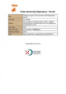
∑ where 𝑓 (𝒙) = 𝒙𝑖 ∈𝑆𝑉𝑠 𝑡𝑖 𝛼𝑖 𝑘(𝒙𝑖 , 𝒙) + 𝑏. Fig. 1 shows the effect of introducing two reject thresholds. Many of the errors caused by the class overlap are rejected. Truly, we can eliminate more errors by enlarging the reject region, but this has a disadvantage of eliminating more correct classification. Thus, we need to find an effective error-reject trade-off. In this paper, we use MI to find the error-reject trade-off. B. MI Measure for Classification Hu et al. [14] presented a systematic study of informationtheoretic measures for classification. They derived the Shannon-based MI measures based on an augmented confusion matrix 𝑪: ⎡ 𝑐 11 ⎢ 𝑐21 ⎢ 𝑪=⎢ . ⎣ . . 𝑐𝑛1
𝑐12 𝑐22 . . . 𝑐𝑛2
... ... .. . ...
𝑐1𝑛 𝑐2𝑛 . . . 𝑐𝑛𝑛
𝑐1(𝑛+1) 𝑐2(𝑛+1) . . . 𝑐𝑛(𝑛+1)
⎤
⎥ ⎥ ⎥, ⎦
where rows represent the true labels and columns represent the predicted labels; 𝑛 is the number of classes; 𝑐𝑖𝑗 represents the number of samples of class 𝑖 classified as class 𝑗; and 𝑛 + 1 represents the reject option. Three features are proposed by them to evaluate a measure for abstaining classification: 1) monotonicity with respect to the diagonal terms of 𝑪; 2) variation with the reject rate; 3) intuitively
0.9
p( z | t=−1) p( z | t=+1) rejects
0.8
conditional density
Supposing that an SVM classifier has been trained on a 𝑑 training set {(𝒙𝑖 , 𝑡𝑖 )}𝑁 𝑖=1 , where 𝒙𝑖 ∈ ℝ and 𝑡𝑖 ∈ {±1}. We use positive to represent class +1 and negative to represent class −1. The decision function of SVMs is [5]: 𝑡𝑖 𝛼𝑖 𝑘(𝒙𝑖 , 𝒙) + 𝑏),
cost matrix cost matrix no cost matrix
⎧ ⎨ +1 0 (𝑟𝑒𝑗𝑒𝑐𝑡) 𝑦= ⎩ −1
A. SVM Classifiers
𝑦 = sgn(
cost matrix
SVMs and the lower and upper reject thresholds respectively are 𝑓− and 𝑓+ (𝑓− ≤ 𝑓+ ), then the decision function is [9]:
III. BACKGROUND
∑
Needed information confidence level cost matrix
0.7 TNR(f−) 0.6
TPR(f ) +
0.5 0.4 RNR(f ,f ) − +
0.3
RPR(f ,f ) − + FPR(f ) +
FNR(f ) −
0.2 0.1
(1)
0 −2
𝒙𝑖 ∈𝑆𝑉𝑠
−1.5
−1
f_
0
f+
1
1.5
2
z
where 𝑘(𝒙𝑖 , 𝒙) is a kernel function and 𝑆𝑉𝑠 represents the set of support vectors. If we introduce the reject option into
Figure 1. The positive and negative class-conditional densities obtained in an artificial dataset.
818
consistent costs among error types and reject types. Based on the above three features, Hu et al. [14] suggested the Shannon-based modified MI 𝐼𝑚 (𝑇 ; 𝑌 ) as the best MI measure for abstaining classification, where 𝑇 denotes the true label; 𝑌 denotes the predicted label and the subscript “m” means modified: 𝐼𝑚 (𝑇 ; 𝑌 ) =
∑∑ 𝑡
𝑦
𝑛 ∑ 𝑛 ∑ 𝑝(𝑡, 𝑦) 𝑐𝑖𝑗 𝑁 𝑐𝑖𝑗 𝑝(𝑡, 𝑦) log , = log ˆ𝑗 𝑝(𝑡)𝑝(𝑦) 𝑁 𝑁𝑖 𝑁 𝑖=1 𝑗=1
Table II T HE AUGMENTED CONFUSION MATRIX OF A BINARY SVM CLASSIFIER WITH REJECT THRESHOLDS 𝑓− AND 𝑓+ . 𝑅𝑁 (𝑓− , 𝑓+ ) IS THE NUMBER OF REJECT NEGATIVES AND 𝑅𝑃 (𝑓− , 𝑓+ ) HAS A SIMILAR MEANING .
True (𝑇 )
(3)
∑𝑛+1 ˆ𝑗 = ∑𝑛 𝑐𝑘𝑗 , 𝑖, 𝑗 = 1, ⋅ ⋅ ⋅ , 𝑛; where 𝑁𝑖 = 𝑘=1 𝑐𝑖𝑘 , 𝑁 𝑘=1 and 𝑁 is the total sample number. Modified MI satisfies the above feature 2) and feature 3) which have been proved in [14]. Although it does not satisfy feature 1), it is also proper to evaluate the abstaining classification results because local minima only occurs in some extreme conditions. Based on their conclusions, Zhang and Hu [15] proposed costfree learning which means getting the optimal classification results without any explicit cost information, and they succeeded to apply it to KNN and Bayesian classifiers. Inspired by their work, we also use modified MI (3) to get the modified-MI-optimal error-reject trade-off for SVMs. The difference between our work and their work is that we apply Newton method for the optimization which is more efficient than Powell’s Algorithm [15]. We have a discussion about cost-free learning and the work of Zhang and Hu [15] in the experimental section. Without ambiguity, we also call “modified MI” MI for simplicity in this paper.
∫
+∞ 𝑓+
(5)
where 𝐼𝑚 (𝑓− , 𝑓+ ) is given by: =
𝐼𝑚 (𝑓− , 𝑓+ ) 𝑇 𝑃 (𝑓+ ) log 𝑁
𝐹 𝑁 (𝑓 ) + 𝑁−
log
+
𝐹 𝑃 (𝑓+ ) 𝑁
log
+
𝑇 𝑁 (𝑓− ) 𝑁
log
(
𝑇 𝑃 (𝑓+ )
𝑃 (+1) 𝑇 𝑃 (𝑓+ )+𝐹 𝑃 (𝑓+ ) 𝐹 𝑁 (𝑓− )
)
(
𝑃 (+1) 𝐹 𝑁 (𝑓− )+𝑇 𝑁 (𝑓− ) 𝐹 𝑃 (𝑓+ )
(
𝑃 (−1) 𝑇 𝑃 (𝑓+ )+𝐹 𝑃 (𝑓+ ) 𝑇 𝑁 (𝑓− )
(
)
(6)
)
𝑃 (−1) 𝐹 𝑁 (𝑓− )+𝑇 𝑁 (𝑓− )
),
where 𝑃 (+1) = 𝑁𝑁+ and 𝑃 (−1) = 𝑁𝑁− are the prior probabilities of classes, where 𝑁+ and 𝑁− are the numbers of positives and negatives respectively (see Table II). In (6), we use the convention that 0 log 0 = 0 and 0 log 00 = 0. In the next section, we introduce Newton method to optimize (6) in order to get the MI-optimal reject thresholds. A. Newton Method According to the definitions of 𝑇 𝑃 𝑅(𝑓+ ), 𝐹 𝑁 𝑅(𝑓− ), 𝐹 𝑃 𝑅(𝑓+ ), and 𝑇 𝑁 𝑅(𝑓− ) (4), their derivatives with respect to 𝑓− and 𝑓+ respectively are: 𝑑𝑇 𝑃 𝑅(𝑓+ ) = −𝜑𝑃 (𝑓+ ); 𝑑𝑓+ 𝑑𝑇 𝑁 𝑅(𝑓− ) = 𝜑𝑁 (𝑓− ); 𝑑𝑓−
𝑑𝐹 𝑃 𝑅(𝑓+ ) = −𝜑𝑁 (𝑓+ ); 𝑑𝑓+ 𝑑𝐹 𝑁 𝑅(𝑓− ) = 𝜑𝑃 (𝑓− ). 𝑑𝑓−
(7)
Taking (4) into (6) and making use of (7), we can get the gradient 𝒈 of 𝐼𝑚 (𝑓− , 𝑓+ ):
𝜑𝑃 (𝑧)d𝑧;
𝒈(1) =
∫
𝑓− 𝐹 𝑁 (𝑓− ) = 𝜑𝑃 (𝑧)d𝑧; 𝑁+ −∞ ∫ +∞ 𝐹 𝑃 (𝑓+ ) 𝐹 𝑃 𝑅(𝑓+ ) = = 𝜑𝑁 (𝑧)d𝑧; 𝑁− 𝑓+ ∫ 𝑓 − 𝑇 𝑁 (𝑓− ) = 𝜑𝑁 (𝑧)d𝑧; 𝑇 𝑁 𝑅(𝑓− ) = 𝑁− −∞ ∫ 𝑓 + 𝑅𝑃 (𝑓− , 𝑓+ ) = 𝜑𝑃 (𝑧)d𝑧; 𝑅𝑃 𝑅(𝑓− , 𝑓+ ) = 𝑁+ 𝑓− ∫ 𝑓 + 𝑅𝑁 (𝑓− , 𝑓+ ) = 𝜑𝑁 (𝑧)d𝑧. 𝑅𝑁 𝑅(𝑓− , 𝑓+ ) = 𝑁− 𝑓−
𝑁+ 𝑁− 𝑁
max 𝐼𝑚 (𝑓− , 𝑓+ ) 𝑠.𝑡. 𝑓− ≤ 𝑓+ ,
We suppose that we have get a trained binary SVM classifier and the augmented confusion matrix is shown in Table II with reject thresholds ( 𝑓− and 𝑓+ (𝑓− ≤) 𝑓+ ). (𝑧) = 𝑝 𝑓 (𝒙) ) = 𝑧∣𝑡 = +1 and Supposing that 𝜑 𝑃 ( 𝜑𝑁 (𝑧) = 𝑝 𝑓 (𝒙) = 𝑧∣𝑡 = −1 respectively are the positive and negative class-conditional densities of SVM outputs, 𝑇 𝑃 𝑅(𝑓+ ) (true positive rate), 𝐹 𝑁 𝑅(𝑓− ) (false negative rate), 𝐹 𝑃 𝑅(𝑓+ ) (false positive rate), 𝑇 𝑁 𝑅(𝑓− ) (true negative rate), 𝑅𝑃 𝑅(𝑓− , 𝑓+ ) (reject positive rate) and 𝑅𝑁 𝑅(𝑓− , 𝑓+ ) (reject negative rate) respectively are (see Fig. 1) [9]: 𝑇 𝑃 (𝑓+ ) = 𝑁+
∑
𝐼𝑚 (𝑓− , 𝑓+ ) to denote 𝐼𝑚 (𝑇 ; 𝑌 ) in order to simplify the expression. According to (3), our objective function is:
IV. MI-O PTIMAL R EJECT RULE FOR SVM
𝑇 𝑃 𝑅(𝑓+ ) =
∑
+1 −1
Predict (𝑌 ) −1 0(𝑅𝑒𝑗𝑒𝑐𝑡) 𝐹 𝑁 (𝑓− ) 𝑅𝑃 (𝑓− , 𝑓+ ) 𝑇 𝑁 (𝑓− ) 𝑅𝑁 (𝑓− , 𝑓+ ) ˆ− 𝑁𝑅 𝑁
+1 𝑇 𝑃 (𝑓+ ) 𝐹 𝑃 (𝑓+ ) ˆ+ 𝑁
∂𝐼𝑚 (𝑓− , 𝑓+ ) ∂𝑓−
𝐹 𝑁 (𝑓− ) ( ) 𝑃 (+1) 𝐹 𝑁 (𝑓− ) + 𝑇 𝑁 (𝑓− ) 𝑇 𝑁 (𝑓− ) ( ); +𝑃 (−1)𝜑𝑁 (𝑓− ) log 𝑃 (−1) 𝐹 𝑁 (𝑓− ) + 𝑇 𝑁 (𝑓− ) ∂𝐼𝑚 (𝑓− , 𝑓+ ) 𝒈(2) = ∂𝑓+ 𝑇 𝑃 (𝑓+ ) ( ) = − 𝑃 (+1)𝜑𝑃 (𝑓+ ) log 𝑃 (+1) 𝑇 𝑃 (𝑓+ ) + 𝐹 𝑃 (𝑓+ ) 𝐹 𝑃 (𝑓+ ) ( ). − 𝑃 (−1)𝜑𝑁 (𝑓+ ) log 𝑃 (−1) 𝑇 𝑃 (𝑓+ ) + 𝐹 𝑃 (𝑓+ ) (8)
𝐹 𝑁 𝑅(𝑓− ) =
=𝑃 (+1)𝜑𝑃 (𝑓− ) log
(4)
When the reject thresholds are 𝑓− and 𝑓+ , we use
819
We further assume that 𝜓𝑃 (𝑧) and 𝜓𝑁 (𝑧) are the derivatives of 𝜑𝑃 (𝑧) and 𝜑𝑁 (𝑧) respectively. Taking the derivatives of (8) with respect to 𝑓− and 𝑓+ again under the help of (4) and (7), we can get the Hessian matrix 𝐻 of 𝐼𝑚 (𝑓− , 𝑓+ ):
Table III C OST MATRIX FOR BINARY ABSTAINING CLASSIFICATION
True (𝑇 )
𝐻(1, 1) 𝐹 𝑁 (𝑓− ) ( ) 𝑃 (+1) 𝐹 𝑁 (𝑓− ) + 𝑇 𝑁 (𝑓− ) 𝑇 𝑁 (𝑓− ) ( ) +𝑃 (−1)𝜓𝑁 (𝑓− ) log 𝑃 (−1) 𝐹 𝑁 (𝑓− ) + 𝑇 𝑁 (𝑓− ) ( )2 𝜑𝑃 (𝑓− )𝑁+ 𝑇 𝑁 (𝑓− ) − 𝜑𝑁 (𝑓− )𝑁− 𝐹 𝑁 (𝑓− ) ( ) ; + 𝑁 ⋅ 𝐹 𝑁 (𝑓− )𝑇 𝑁 (𝑓− ) 𝐹 𝑁 (𝑓− ) + 𝑇 𝑁 (𝑓− ) 𝐻(2, 2) 𝑇 𝑃 (𝑓+ ) ( ) = − 𝑃 (+1)𝜓𝑃 (𝑓+ ) log 𝑃 (+1) 𝐹 𝑃 (𝑓+ ) + 𝑇 𝑃 (𝑓+ ) 𝐹 𝑃 (𝑓+ ) ( ) −𝑃 (−1)𝜓𝑁 (𝑓+ ) log 𝑃 (−1) 𝐹 𝑃 (𝑓+ ) + 𝑇 𝑃 (𝑓+ ) ( )2 𝜑𝑃 (𝑓+ )𝑁+ 𝐹 𝑃 (𝑓+ ) − 𝜑𝑁 (𝑓+ )𝑁− 𝑇 𝑃 (𝑓+ ) ( ) ; + 𝑁 ⋅ 𝐹 𝑃 (𝑓+ )𝑇 𝑃 (𝑓+ ) 𝐹 𝑃 (𝑓+ ) + 𝑇 𝑃 (𝑓+ ) 𝐻(1, 2) = 𝐻(2, 1) = 0;
+1 −1
+1 0 1
Predict (𝑌 ) −1 0(𝑅𝑒𝑗𝑒𝑐𝑡) 𝐶𝐹 𝑁 𝐶𝑅𝑃 0 𝐶𝑅𝑁
=𝑃 (+1)𝜓𝑃 (𝑓− ) log
Similar to the derivation of the gradient and Hessian matrix of 𝐼𝑚 (𝑓− , 𝑓+ ), the gradient 𝒈 𝑒𝑐 of 𝐸𝐶(𝑓− , 𝑓+ ) is: ∂𝐸𝐶(𝑓− , 𝑓+ ) ∂𝑓− =𝑃 (+1)𝜑𝑃 (𝑓− )(𝐶𝐹 𝑁 − 𝐶𝑅𝑃 ) − 𝑃 (−1)𝜑𝑁 (𝑓− )𝐶𝑅𝑁 ; ∂𝐸𝐶(𝑓− , 𝑓+ ) 𝒈 𝑒𝑐 (2) = ∂𝑓+ =𝑃 (+1)𝜑𝑃 (𝑓+ )𝐶𝑅𝑃 + 𝑃 (−1)𝜑𝑁 (𝑓+ )(𝐶𝑅𝑁 − 1); (13) 𝒈 𝑒𝑐 (1) =
(9)
the Hessian matrix 𝐻𝑒𝑐 of 𝐸𝐶(𝑓− , 𝑓+ ) is: 𝐻𝑒𝑐 (1, 1) = 𝑃 (+1)𝜓𝑃 (𝑓− )(𝐶𝐹 𝑁 − 𝐶𝑅𝑃 ) − 𝑃 (−1)𝜓𝑁 (𝑓− )𝐶𝑅𝑁 ; 𝐻𝑒𝑐 (2, 2) = 𝑃 (+1)𝜓𝑃 (𝑓+ )𝐶𝑅𝑃 + 𝑃 (−1)𝜓𝑁 (𝑓+ )(𝐶𝑅𝑁 − 1); 𝐻𝑒𝑐 (1, 2) = 𝐻𝑒𝑐 (2, 1) = 0.
where we use the convention that 00 = 0. We want to use Newton method to optimize (5), but we have no idea of the values of 𝜑𝑃 (𝑧), 𝜑𝑁 (𝑧), 𝜓𝑃 (𝑧) and 𝜓𝑁 (𝑧). Fortunately, we can estimate them from the training set using Parzen Window method [16]. With the help of Parzen Window method, we can apply Newton method to optimize problem (5): −1 (𝑓− , 𝑓+ )𝑇𝑘 = (𝑓− , 𝑓+ )𝑇𝑘−1 + 𝛼𝐻𝑘−1 𝒈 𝑘−1 ,
(14)
In fact, given a cost matrix, we can also use Newton method to minimize the expected classification cost (12). However, this approach has a drawback of re-optimization if the cost matrix is changed while in such condition, the optimization method based on ROC analysis [9] can get the optimal reject thresholds directly from the estimated ROC curve. We use 𝒈 𝑒𝑐 to calculate the cost information embedded in maximizing 𝐼𝑚 (𝑓− , 𝑓+ ). We assume that the solution of problem (5) ∗ ∗ 𝑇 , 𝑓+ ) . Because there are three variables in the cost is (𝑓− matrix, we have to provide a constraint among 𝐶𝐹 𝑁 , 𝐶𝑅𝑃 and 𝐶𝑅𝑁 in order to obtain a unique solution. We consider two kinds of constraints here, one is 𝐶𝑅𝑁 = 𝐶𝑅𝑃 and the other is 𝐶𝑅𝑁 = 𝜂, 𝜂 is a given constant (0 < 𝜂 < 1). Then we can obtain the solutions of 𝐶𝐹 𝑁 , 𝐶𝑅𝑃 and 𝐶𝑅𝑁 by solving 𝒈 𝑒𝑐 ∣(𝑓− ,𝑓+ )𝑇 =(𝑓−∗ ,𝑓+∗ )𝑇 = 0 with one of the above constraints. If the constraint is 𝐶𝑅𝑁 = 𝐶𝑅𝑃 , then the solutions are:
(10)
where 𝛼 is the learning rate. Newton method has the property of quadratic convergence and in our experiments, the optimization usually converges around six iterations. V. T HE E MBEDDED C OST I NFORMATION Cost-sensitive learning is very popular in abstaining classification and the expected classification cost is usually minimized through ROC analysis [3], [9]. The main problem with cost-sensitive learning is unavailability of proper cost information about misclassification and rejection. We think that there is cost information embedded in maximizing 𝐼𝑚 (𝑓− , 𝑓+ ). As the cost matrix has the properties of scaling invariance and shifting invariance [17], it can be normalized to the one shown in Table III. The elements in the cost matrix should satisfy the following constraints [3] so that the reject option is applicable: ⎧ ⎨ 0 < 𝐶𝑅𝑃 < 𝐶𝐹 𝑁 ; 0 < 𝐶𝑅𝑁 < 1; ⎩ 𝐶𝑅𝑃 + 𝐶𝑅𝑁 ⋅ 𝐶𝐹 𝑁 < 𝐶𝐹 𝑁.
⎧ ⎨ 𝐶𝑅𝑁 = 𝐶𝑅𝑃 = ⎩ 𝐶𝐹 𝑁 = 𝐶𝑅𝑃 +
∗ 𝑃 (−1)𝜑𝑁 (𝑓+ ) ∗ )+𝑃 (−1)𝜑 (𝑓 ∗ ) ; 𝑃 (+1)𝜑𝑃 (𝑓+ 𝑁 + ∗ 𝑃 (−1)𝜑 (𝑓− ) . 𝐶𝑅𝑃 ⋅ 𝑃 (+1)𝜑𝑁 ∗ 𝑃 (𝑓− )
(15)
If the constraint is 𝐶𝑅𝑁 = 𝜂, 0 < 𝜂 < 1, then the solutions are: ⎧ 𝑃 (−1)𝜑 (𝑓 ∗ ) ⎨ 𝐶𝑅𝑃 = (1 − 𝜂) ⋅
(11)
⎩ 𝐶𝐹 𝑁 = 𝐶𝑅𝑃 +
𝑁
+
;
∗) 𝑃 (+1)𝜑𝑃 (𝑓+ ∗ 𝑃 (−1)𝜑𝑁 (𝑓− ) 𝜂 ⋅ 𝑃 (+1)𝜑𝑃 (𝑓 ∗ ) . −
(16)
The above embedded cost information is important to us. Firstly, it establishes the relationship between our MI-based reject rule and cost-sensitive learning. Secondly, if we are unsatisfied with the abstaining classification results of our MI-based reject rule, we can choose the proper cost information for practical requirements based on this embedded
Then the expected classification cost is: 𝐸𝐶(𝑓− , 𝑓+ ) =𝑃 (+1) ⋅ 𝐹 𝑁 𝑅(𝑓− ) ⋅ 𝐶𝐹 𝑁 + 𝑃 (+1) ⋅ 𝑅𝑃 𝑅(𝑓− , 𝑓+ ) ⋅ 𝐶𝑅𝑃 +𝑃 (−1) ⋅ 𝐹 𝑃 𝑅(𝑓+ ) + 𝑃 (−1) ⋅ 𝑅𝑁 𝑅(𝑓− , 𝑓+ ) ⋅ 𝐶𝑅𝑁. (12)
820
cost information, and then use cost-sensitive learning [3], [9] to re-optimize the reject thresholds. Because we use the abstaining classification results to calculate the cost information which is an inverse process of cost-sensitive learning, the obtained embedded cost information always satisfies the constraints (11). A. Relation between Two Reject Rules In [23], Hu systematically describes the relationship between Bayesian classifiers and MI classifiers which helps us understand classification from MI perspective. Under his framework, we briefly describe the relationship between our MI-based reject rule and the reject rule of Grandvalet et al. [10] through the embedded cost information (Table III). The abstaining decision function in [23] is: ⎧ ⎨ +1 0 (𝑟𝑒𝑗𝑒𝑐𝑡) 𝑦= ⎩ −1
if 𝑝(+1∣𝒙) ≥ 1 − 𝑇𝑟2 , if 𝑇𝑟1 ≤ 𝑝(+1∣𝒙) < 1 − 𝑇𝑟2 , if 𝑝(+1∣𝒙) < 𝑇𝑟1 ,
Figure 2. Graphical descriptions of dual double-hinge losses (modified based on [10]). Table IV C HARACTERISTICS OF THE REAL - WORLD DATASETS
(17)
where 𝑇𝑟1 and 𝑇𝑟2 are two thresholds which reflect Chow’s reject rule [2]. 𝑇𝑟1 , 𝑇𝑟2 > 0 and 0 < 𝑇𝑟1 + 𝑇𝑟2 ≤ 1 [23] so that the rejection is applicable. They can be computed using the embedded cost information in Table III: 𝑇𝑟1 =
𝐶𝑅𝑁 𝐶𝑅𝑃 , 𝑇𝑟2 = . 𝐶𝑅𝑁 + 𝐶𝐹 𝑁 − 𝐶𝑅𝑃 𝐶𝑅𝑃 + 1 − 𝐶𝑅𝑁
Dataset WDBC Pima German Credit KC1 Mammography
VI. E XPERIMENTS We implement the experiments with the help of libsvm [18]. Table IV presents the characteristics of the real-world datasets. KC11 is from the domain of software engineering measurements; Mammography was generously provided by Dr. Nitesh Chawla [19]; and the remaining three datasets are from the UCI data repository. To reduce the bias in comparison, we use 10-fold cross-validation in all the datasets. In each of the runs, we select 60% of the whole dataset as the training set, 20% as the validation set and the remaining 20% as the test set. For imbalanced dataset, positive denotes the minority class and negative denotes the majority class. Although in some imbalanced datasets there are only a few positives in the validation set, experimental results show that Newton method can also converge. Firstly, the original nonabstaining classification results are presented in order to show the merits of abstaining classification. Secondly, to evaluate the effectiveness of our
𝑙+ = max{−(1 − 𝑇𝑟1 )𝑓 (𝒙) + 𝐻(𝑇𝑟1 ), −𝑇𝑟2 𝑓 (𝒙) + 𝐻(1 − 𝑇𝑟2 ), 0}, (19)
where 𝐻(𝑞) = −𝑞 log(𝑞)−(1−𝑞) log(1−𝑞). And the corresponding reject thresholds (𝑓− , 𝑓+ )𝑇 of SVM is computed as follows: (20)
Along the 𝑓 (𝒙) axis, the two hinge points 𝑓1 and 𝑓2 , and another point 𝑓3 respectively are: 𝑓1 =𝑓− + 𝑓3 =
log(1 − 𝑇𝑟1 ) log(1 − 𝑇𝑟2 ) , 𝑓 2 = 𝑓+ − , 𝑇𝑟1 𝑇𝑟2
−𝑇𝑟1 𝑓− − 𝑇𝑟2 𝑓+ + log 1 − 𝑇𝑟1 − 𝑇𝑟2
1−𝑇𝑟2 1−𝑇𝑟1
# of Features 30 8 24 21 6
region without penalty 𝑓 (𝒙) ≥ 𝑓2 . The correct region with penalty is necessary for a unique classification solution. From the constraint 0 < 𝑇𝑟1 + 𝑇𝑟2 ≤ 1, we can easily 1 2 1 2 ) ≥ 𝑎𝑏𝑠(𝑘− ) and 𝑎𝑏𝑠(𝑘+ ) ≥ 𝑎𝑏𝑠(𝑘+ ) verify that 𝑎𝑏𝑠(𝑘− which indicate that a misclassification will cost more than a reject in the same class. The above is a typical relationship between our MI-based reject rule and another reject rule through the embedded cost information.
𝑙− = max{𝑇𝑟1 𝑓 (𝒙) + 𝐻(𝑇𝑟1 ), (1 − 𝑇𝑟2 )𝑓 (𝒙) + 𝐻(1 − 𝑇𝑟2 ), 0},
𝑇𝑟1 1 − 𝑇𝑟2 ), 𝑓+ = log( ). 1 − 𝑇𝑟1 𝑇𝑟2
# of Positive Samples(%) 212 (37.26) 268 (34.90) 300 (30.00) 326 (15.46) 260 (2.33)
(18)
Grandvalet et al. [10] built up abstaining SVM classifiers based on a probabilistic interpretation of SVM that the hinge loss can be viewed as a relaxed minimization of negative log-likelihood. Thus, instead of estimating 𝑝(+1∣𝒙) in the whole range, they believe that the estimation of 𝑝(+1∣𝒙) can only be accurate in the vicinity of 𝑇𝑟1 and 𝑇𝑟2 . Fig. 2 intuitively shows the relationship between MI-based reject rule and the reject rule of Grandvalet et al. [10]. The loss functions of negatives and positives, which are used in the reject rule of Grandvalet et al., are different that we redefine as “dual double-hinge losses”:
𝑓− = log(
# of Samples 569 768 1000 2109 11180
(21)
.
Within each double-hinge loss function, e.g. 𝑙+ , four regions are formed along the 𝑓 (𝒙) axis with different meanings, namely, error region 𝑓 (𝒙) < 𝑓− , reject region 𝑓− ≤ 𝑓 (𝒙) < 𝑓+ , correct region with penalty 𝑓+ ≤ 𝑓 (𝒙) < 𝑓2 and correct
1 http://promise.site.uottawa.ca/SERepository/datasets-page.html
821
MI-based reject rule, we choose Chow’s reject rule and MIbased cross-validation reject rule (MICVR) as baselines. We apply Chow’s reject rule after mapping SVM outputs into posterior probabilities using Platt’s method [12] and we set the “rejection threshold” of Chow’s reject rule as 0.4 [2]. MICVR is doing cross-validation based on MI to select the optimal reject thresholds. In our MI-based reject rule, during the optimization of (5), we randomly choose the initial points around zero several times and then pick the reject thresholds with the highest MI. There are two reasons that we do not compare our MI-based reject rule with the reject rules based on cost-sensitive learning. One is that we assume that there is no cost information at hand, the other is that our MI-based reject rule is related to cost-sensitive learning which will be experimentally discussed in the following section.
double-hinge losses used in the reject rule of Grandvalet et al. [10]. B. Abstaining Classification Results As far as we know, there is no general measure to evaluate abstaining classification until now. We apply normalized MI (NMI) to evaluate the abstaining classification results which is proposed by Hu et al. [14] and is used in [15]. NMI is the ratio of MI over the entropy of true class distributions which is a constant. Besides NMI, we also use error rate and reject rate to reflect the error-reject trade-off; FNR, RPR and precision to evaluate the classification of positives. Table V shows the experimental classification results. Firstly, the error rates of abstaining classification are smaller than nonabstaining classification thanks to the reject option. As a result, we can make less wrong predictions in reality and make more careful predictions of those rejected instances by further investigation. Besides, in the imbalanced datasets like KC1 and Mammography where we care more about the positive classification, abstaining classification reduces FNRs through proper RPRs and improves precisions of positive classification. Secondly, in terms of NMI, Chow’s reject rule performs the worst among all the classification methods. In the balanced datasets, WDBC and Pima, compared with our MI-based reject rule, Chow’s reject rule has higher error rates but lower reject rates, and we can choose one of them based on practical requirements. While in the imbalanced datasets, KC1 and Mammography, error rate is insufficient to evaluate the classification results, and people concern more with positive classification. Although RPRs of our reject rule are higher, FNRs of our reject rule are much smaller than Chow’s reject rule. Thus our reject rule would rather reject a positive instance than make a wrong positive classification. In fact, in imbalanced datasets, Chow’s reject rule even performs worse than nonabstaining classification. This is because the performance of Chow’s reject rule depends on the estimation of posterior probability [20] which is seldom sufficiently accuracy. Above all, our MI-based reject rule can give reasonable abstaining classification results in both balanced and imbalanced datasets. Thirdly, the purpose of making comparison between MICVR and our MI-based reject rule is to evaluate the efficiency of Newton method. We use student test with unequal variance at the 1% significance level [21] to test the difference of NMI between these two reject rules. The result is that there is no statistical difference between them which reflects that Newton method is efficient in optimizing (5). Except in the German Credit and KC1 datasets, the reject thresholds of MICVR and our MI-based reject rule are very close. In our experiments, Newton method usually converges around six iterations which is computationally efficient while MICVR has a heavy time complexity,
A. An Illustrative Example We give a toy example of MI-based reject rule in Fig. 3(a) where the classes are balanced. Because of noise, instances around the decision boundary of SVM are more prone to be misclassified which had better better been rejected for further investigation. After using MI-based reject rule in this artificial dataset, we obtain two reject thresholds 𝑓+ = 0.6470 and 𝑓− = −0.5609. We can easily find that these two reject thresholds just locate on the places that all the misclassifications are rejected. It intuitively shows the effectiveness of MI-based reject rule in finding the reasonable error-reject tradeoff. The embedded cost information with constraint 𝐶𝑅𝑃 = 𝐶𝑅𝑁 is 𝐶𝐹 𝑁 = 1.0050 and 𝐶𝑅𝑃 = 𝐶𝑅𝑁 = 0.3883. And Fig. 3(b) shows the dual
Original Boundary Reject Boundaries
0
0.64704
−0.56091
2 1.5 1 X2
0.5 0 −0.5
−1
−0.5
0
−1.5
0 X1
0.64704
−0.56091
−1 −1.5
0.5
1
1.5
(a) log(1+exp(f(x))) negative loss log(1+exp(−f(x))) positive loss
2 1.8 1.6
loss
1.4 1.2 1 0.8 0.6 0.4 0.2 0 −1.73
−1
−0.46−0.01 0.45
1.72
f(x)
(b) Figure 3. (a) A toy example of reject boundaries of MI-based reject rule; (b) The dual double-hinge loss functions of Grandvalet et al. [10].
822
Table V A BSTAINING CLASSIFICATION RESULTS OF THREE REJECT RULES AND NONABSTAINING CLASSIFICATION RESULTS OF SVM. T HE NUMBER BELOW THE DATASET IS THE RATIO OF POSITIVES OVER NEGATIVES . MEAN ( STD )
Dataset WDBC (1:1.68)
Pima (1:1.87)
German Credit (1:2.33)
KC1 (1:5.47)
Mammography (1:42)
Method
NMI
Chow’s MICVR Ours NC Chow’s MICVR Ours NC Chow’s MICVR Ours NC Chow’s MICVR Ours NC Chow’s MICVR Ours NC
0.8526(0.0558) 0.8776(0.0508) 0.8971(0.0479) 0.8293(0.0888) 0.1796(0.0038) 0.2414(0.0456) 0.2491(0.0416) 0.1808(0.0567) 0.1167(0.0493) 0.1631(0.0413) 0.1665(0.0441) 0.1306(0.0437) 0.0074(0.0045) 0.1617(0.0376) 0.1589(0.0399) 0.1182(0.0378) 0.1853(0.0456) 0.4947(0.0403) 0.5026(0.0429) 0.4373(0.0342)
Error Rate(%) 2.00(0.93) 1.07(0.97) 0.88(0.70) 2.73(1.60) 20.07(2.16) 16.42(4.98) 16.41(3.89) 25.83(2.73) 19.62(3.22) 21.78(5.14) 20.48(2.87) 27.78(3.30) 12.86(0.74) 26.11(6.28) 22.79(3.69) 28.47(2.15) 1.67(0.15) 2.33(0.58) 2.35(0.38) 4.67(0.34)
Reject Rate(%) 1.38(1.24) 5.59(5.06) 4.30(2.61) —— 17.14(3.15) 34.28(10.83) 31.13(6.15) —— 18.44(3.43) 36.37(11.37) 21.06(5.62) —— 8.02(2.27) 27.20(10.02) 24.12(4.44) —— 0.72(0.22) 8.18(2.39) 6.20(1.15) ——
FNR(%)
RPR(%)
Precision(%)
2.55(1.96) 1.94(2.07) 1.89(1.71) 3.30(2.76) 30.59(4.99) 9.13(6.13) 9.24(4.36) 26.45(8.99) 42.00(6.26) 13.00(7.24) 25.67(5.70) 32.59(6.45) 76.08(6.16) 8.35(3.37) 12.34(4.65) 29.36(7.03) 58.08(6.03) 9.06(4.41) 9.96(4.50) 15.13(3.47)
1.51(1.87) 3.70(4.06) 3.45(3.11) —— 22.31(6.10) 36.42(13.45) 34.59(9.72) —— 31.15(9.09) 34.63(13.90) 23.22(6.90) —— 23.58(5.99) 27.20(15.55) 32.97(7.47) —— 14.66(5.17) 16.37(4.83) 13.55(3.93) ——
97.30(2.28) 99.16(1.74) 99.62(0.90) 96.09(2.96) 73.80(6.62) 72.46(8.04) 71.29(5.96) 61.24(2.31) 70.69(12.44) 61.76(7.97) 64.68(5.80) 53.12(4.52) 10.74(23.88) 34.83(5.04) 35.75(3.69) 31.36(2.55) 68.06(8.22) 48.41(6.46) 47.86(4.22) 31.45(1.79)
Table VI T HE EMBEDDED COST INFORMATION . T HE NUMBER BESIDE THE DATASET IS THE RATIO OF POSITIVES OVER NEGATIVES . MEAN ( STD )
Dataset WDBC(1:1.68) Pima(1:1.87) German Cr.(1:2.33) KC1(1:5.47) Mammography(1:42)
Constraint: CRP=CRN CFN CRP=CRN 1.701(0.896) 0.290(0.065) 2.612(0.706) 0.480(0.039) 2.573(0.231) 0.548(0.036) 8.551(0.924) 0.758(0.015) 85.77(12.23) 0.836(0.016)
Reject Thresholds [𝑓− , 𝑓+ ]𝑇 [−0.1056(0.0211), 0.1097(0.0216)]𝑇 [−0.3636(0.3640), 0.2271(0.1373)]𝑇 [−0.2958(0.1927), 0.2236(0.1039)]𝑇 —— [0.0890(0.0240), 0.6921(0.0369)]𝑇 [−0.6591(0.2343), 0.5182(0.2976)]𝑇 [−0.5692(0.1533), 0.4753(0.1342)]𝑇 —— [0.2046(0.0272), 0.8373(0.0679)]𝑇 [−0.6629(0.2482), 0.3218(0.2258)]𝑇 [−0.1854(0.0922), 0.3603(0.0887)]𝑇 —— [1.0085(0.0510), 1.6862(0.0827)]𝑇 [−0.8644(0.1277), 0.2636(0.4415)]𝑇 [−0.5913(0.0890), 0.4496(0.1134)]𝑇 —— [1.3597(0.0631), 1.7746(0.0789)]𝑇 [−0.6496(0.2204), 0.6382(0.1794)]𝑇 [−0.5091(0.1087), 0.5837(0.0901)]𝑇 ——
information can help us find the reasonable cost information more easily and quickly.
Constraint: CRN=0.4 CFN CRP 2.200(0.883) 0.253(0.075) 2.218(0.372) 0.540(0.079) 2.257(0.230) 0.737(0.098) 6.077(0.818) 1.867(0.159) 44.29(5.193) 3.160(0.429)
D. Discussion By making comparison with Chow’s reject rule and MICVR, we come to the conclusion that our MI-based reject rule can give reasonable abstaining classification results and Newton method is efficient in optimizing (5). Zhang and Hu proposed cost-free learning in [15] which is to learn to get the optimal classification results without using any explicit cost information. It is easy to verify that our MIbased reject rule is a kind of cost-free learning. From another perspective, we can view cost-free learning as cost-sensitive learning with embedded cost information. It is pointed out that the embedded cost information can be derived by analysing the relationship between cost-free learning and cost-sensitive learning which has already been shown in Section V and in [15]. We are not sure that whether abstaining classification results of cost-free learning satisfy practical requirements, but its embedded cost information could help us to find the proper cost information more easily and quickly. Overall, cost-sensitive learning is more flexible and powerful. However, as Hu [23] said, cost-free learning was proposed to enrich the content of cost-sensitive learning and let us understand cost-sensitive learning from a different viewpoint. Furthermore, we can let the data speak for themselves firstly and then embed our prior knowledge into the classifiers. In this paper, we extend cost-free learning from KNN and Bayesian classifiers [15] to SVM which is more popular in classification. Besides, compared with Powell’s algorithm
especially when the search interval becomes larger and the step size becomes smaller.
C. The Results of Embedded Cost Information In Section V, we have discussed that there is cost information embedded in maximize 𝐼𝑚 (𝑓− , 𝑓+ ). Table VI shows the results of embedded cost information with constraints 𝐶𝑅𝑃 = 𝐶𝑅𝑁 and 𝐶𝑅𝑁 = 0.4. It is verified that all the cost matrices satisfy constraints (11). Moreover, given an embedded cost matrix, if we use Newton method proposed in Section V to minimize (12), we will get the same reject thresholds. From the results of embedded cost information with constraint 𝐶𝑅𝑁 = 0.4, we find that the negative misclassification cost may be lower than the positive rejection cost which, we think, sometimes is rational. If the abstaining classification results of our MI-based reject rule do not meet the practical requirements, we can estimate the cost matrix based on the embedded cost information and then use cost-sensitive learning to get the optimal reject thresholds. In all, this embedded cost
823
used by Zhang and Hu [15], Newton method is more efficient for the optimization.
[8] G. Fumera, F. Roli, “Support vector machines with embedded reject option,” Pattern Recognition with Support Vector Machines, pp. 68–82, 2002.
VII. C ONCLUSION The reject option is a key option in classification where errors cause severe losses. Then the rejected samples can be classified more carefully. Ferri et al. [22] have used this principle to build delegating classifiers. In this paper, we extend the cost-free learning of Zhang and Hu [15] to SVM and develop a novel MI-based reject rule for SVM which is a method of post-processing. We derive the gradient and Hessian matrix of MI between the true labels and the predicted labels so that Newton method, which is more efficient than Powell’s algorithm, can be used to optimize the MI-based objective function. Besides, we also obtain the cost information embedded in MI which reflects the relationship between our MI-based reject rule and cost-sensitive learning, and furthermore, if the abstaining classification results of our MI-based reject rule are not satisfied, the embedded cost information can help us find the proper cost information that meets the practical requirements more easily and quickly. Conventional measures for classification such as G-mean and F-measure can not be used to evaluate abstaining classification because the reject option is neglected by them. In the future, we will further investigate how to properly evaluate abstaining classification results.
[9] F. Tortorella, “Reducing the classification cost of support vector classifiers through an ROC-based reject rule,” Pattern Analysis & Applications, Vol. 7, No. 2, pp. 128–143, July 2004. [10] Y. Grandvalet, A. Rakotomamonjy, J. Keshet, S. Canu, “Support vector machines with a reject option,” Advances in Neural Information Processing Systems, pp. 537–544, 2009. [11] J. C. Principe, Information theoretic learning: Renyi’s entropy and kernel perspectives, Springer, 2010. [12] J. C. Platt, “Probabilistic outputs for support vector machines and comparisons to regularized likelihood methods,” In Proceedings of Advances in Large Margin Classifiers, Vol. 10, No. 3, pp. 61–74, MIT Press, 1999. [13] P. L. Bartlett, M. H. Wegkamp, “Classification with a reject option using a hinge loss,” Journal of Machine Learning Research, Vol. 9, pp. 1823–1840, June 2008. [14] B.G. Hu, R. He, X.T. Yuan, “Information-theoretic measures for objective evaluation of classifications,” Acta Automatica Sinica, Vol. 38, No. 7, pp. 1169–1182, July 2012. [15] X.W. Zhang, B.G. Hu, “Learning in the class imbalance problem when costs are unknown for errors and rejects,” 12th International Conference on Data Mining Workshops, pp. 194– 201, 2012.
ACKNOWLEDGMENT Thanks the anonymous reviewers for their valuable comments to improve the paper. This work is supported by NSFC grants #61075051 and #61273196.
[16] E. Parzen, “On estimation of a probability density function and mode,” The Annals of Mathematical Statistics, Vol. 33, No. 3, pp. 1065–1076, Sept. 1962.
R EFERENCES
[17] C. Elkan, “The foundations of cost-sensitive learning,” International Joint Conference on Artificial Intelligence, pp. 973– 978, 2001.
[1] C. Ferri, J. Hern´andez-Orallo, “Cautious classifiers,” In Proceedings of the 1st International Workshop on ROC Analysis in Artificial Intelligence, pp. 27–36, 2004.
[18] C.C. Chang, C.J. Lin, “LIBSVM: a library for support vector machines,” ACM Transactions on Intelligent Systems and Technology, Vol. 2, No. 27, pp. 1–27, April 2011.
[2] C. Chow, “On optimum recognition error and reject tradeoff,” IEEE Transactions on Information Theory, Vol. 16, No. 1, pp. 41–46, Jan. 1970.
[19] N. V. Chawla, K. W. Bowyer, T. E. Moore, W. P. Kegelmeyer, “SMOTE: synthetic minority over-sampling technique,” Journal Of Artificial Intelligence Research, Vol. 16, pp. 321–357, June 2002.
[3] T. Pietraszek, “Optimizing abstaining classifiers using ROC analysis,” In Proceedings of International Conference on Machine Learning, pp. 665–672, 2005. [4] C. Friedel, U. R¨uckert, S. Kramer, “Cost curves for abstaining classifiers,” In Proceedings of the ICML 2006 Workshop on ROC Analysis in Machine Learning, pp. 33–40, 2006.
[20] G. Fumera, F. Roli, G. Giacinto, “Reject option with multiple thresholds,” Pattern Recognition, Vol. 33, No. 12, pp. 2099– 2101, March 2000.
[5] V. Vapnik, The nature of statistical learning theory, 1st ed., Springer-Verlag New York, New York, 1995.
[21] E. L. Lehmann, J. P. Romano, Testing statistical hypotheses, Springer, New York, 2005.
[6] J. Shawe-Taylor, “Classification accuracy based on observed margin,”, Algorithmica, Vol. 22, No. 1–2, pp. 157–172, Springer, Sept. 1998.
[22] C. Ferri, P. Flach, J. Hern´andez-Orallo, “Delegating classifiers,” In Proceedings of the 21st International Conference on Machine Learning, 2004.
[7] S. Mukherjee, P. Tamayo, D. Slonim, A. Verri, T. Golub, J. Mesirov, T. Poggio, “Support vector machine classification of microarray data,” AI Memo 1677, Massachusetts Institute of Technology, 1999.
[23] B.G. Hu, “What are the differences between Bayesian classifiers and mutual-information classifiers?,” IEEE Transactions on Neural Networks and Learning Systems, August 2013, in press.
824