I. INTRODUCTION
Costas Arrays, Number of Hops, and Time-Bandwidth Product KEN TAYLOR, Member, IEEE SCOTT RICKARD, Senior Member, IEEE KONSTANTINOS DRAKAKIS, Senior Member, IEEE University College Dublin
In this work we consider the impact of the number of hops of a frequency hopped code on the auto-correlation surface it produces. The analysis focuses on Costas arrays, which are frequency hopped codes possessing ideal auto-correlation properties. There are two common choices for the number of hops, the minimal sidelobe region (MSR) choice, and the Nyquist choice. We propose two new methods, minimize maximal sidelobe (MMS), and minimize maximum peak sidelobe (MMPS).
Manuscript received August 26, 2011; released for publication January 19, 2012. IEEE Log No. T-AES/49/3/944626. Refereeing of this contribution was handled by J. Taque. This material is based upon works supported by the Science Foundation Ireland under Grant 05/YI2/I677, 06/MI/006 (Claude Shannon Institute), and 08/RFP/MTH1164. Authors’ current addresses: K. Taylor and S. Rickard, Complex and Adaptive Systems Laboratory, School of Electrical Electronic and Mechanical Engineering, University College Dublin, Block 8, Belfield Office Park, Clonskeagh,Dublin 4, Ireland, E-mail: (
[email protected]); K. Drakakis, International Investment and Underwriting, Ireland.
c 2013 IEEE 0018-9251/13/$26.00 °
The performance of frequency hopped codes used in RADAR and SONAR is dependent on the auto/cross-ambiguity properties of the signals. By examining the relationship between mainlobe and sidelobe peaks, the accuracy of signal detection can be determined. Costas arrays [1—3] provide a suitable choice for a frequency hopped code due to their nearly ideal auto-ambiguity properties. The center of the auto-correlation surface for a Costas array contains a narrow spike, the mainlobe. The narrowness of this spike in time/frequency determines the range/Doppler resolution of the signal. The peaks away from the mainlobe, the sidelobes, can cause false detections. In this work we examine the relationship between number of hops (N), time-bandwidth product (TB) and signal performance. Our measure of signal performance used here is the maximum sidelobe to mainlobe ratio. The goal is to determine how to choose the value of N that optimizes performance. We initially consider the auto-correlation surface in time only first, without the Doppler shift, and then we examine the effect when it is included. The analysis is made more tractable by partitioning the auto-ambiguity surface into two regions: the mainlobe region and the sidelobe region. Ultimately, the waveform performance is determined by the choice of coding scheme and the relationship of N to TB. There are two choices of N to TB relationship that are popular in the literature. The first, the minimal sidelobe region (MSR) choice described in Titlebaum [4], optimizes the performance in the sidelobe region. This choice unfortunately sacrifices the performance in the mainlobe region. The second, commonly called the Nyquist choice, has slightly worse sidelobe region performance, but exhibits much cleaner mainlobe region behavior. Beginning with a zero Doppler analysis, for a constant bandwidth, we vary the number of hops and empirically determine the size of sidelobes in the mainlobe and sidelobe regions. Our results show that, as the number of hops increases, the size of the largest sidelobe in the mainlobe region falls dramatically and then levels off, while the size of the largest sidelobe region peak increases steadily. The crossover point for these trends yields a suggested number of hops (the minimize maximal sidelobe (MMS) choice), and we compare this choice to the MSR and Nyquist methods. We also determine the best choice when center region behavior is a priority (the MMPS choice). Both the MMS and MMPS choices are, in general, within +=¡ one hop of the Nyquist choice. Performance only degrades slightly with increasing number of hops (larger than the Nyquist choice), which is useful for applications where a larger number of hops is desirable (e.g., when a larger number of hopping sequences are needed).
IEEE TRANSACTIONS ON AEROSPACE AND ELECTRONIC SYSTEMS VOL. 49, NO. 3
JULY 2013
1995
Fig. 1. Thumbtack auto-correlation surface.
We then assess the impact of including Doppler shift in the analysis. Once again for constant bandwidth we vary the number of hops and examine trends in the size of sidelobes in both regions. These results are compared with existing results in [3]. In the MMS case the results show that the crossover point occurs at a much larger value than suggested by the Nyquist choice. For the minimize maximal peak sidelobe (MMPS) choice, the maximum mainlobe correlation decreases with increasing N. Therefore N ! 1 in the MMPS case. The organization of the paper is as follows. Section II gives a brief history of Costas arrays. Section III gives a brief introduction to finite fields, then details the two main methods of generating Costas arrays. These methods are then compared with each other and other generation techniques. Section IV examines the auto-correlation surface by splitting it into two separate regions, the mainlobe region and the sidelobe region. Section V examines waveform performance based on the choice of N to TB relationship. Existing choices are reviewed, and then compared with new results. II. ORIGIN OF COSTAS ARRAYS RADAR and SONAR systems determine the location of targets and the (radial) velocity at which they are traveling by periodically transmitting a waveform W and listening for reflections R. In an ideal environment, R is a copy of W, only attenuated and shifted in frequency and time. The time delay can be used to determine the distance to the target, while the frequency shift gives relative velocity via the Doppler effect. Consider using a matched filter in a SONAR setting to detect the time and frequency shifts: R is cross-correlated with shifted versions of W for various time and frequency shifts, and the filter looks for those shifts yielding maximal cross-correlation. In practice, this idea proved unsuccessful. The incoherent ocean environment introduces small phase errors which are frequency dependent [1]. The received waveform is thus no longer a shifted copy of W, and coherent processing techniques suffer poor performance due to destructive self-interference arising from the phase changes. 1996
J. P. Costas’s idea [1] was to discard the unreliable phase information, and instead examine cross-correlations of the energy contents of W and R alone. Costas arrays are matrices of zeros and ones, commonly depicted by blanks and dots, respectively, on an N-by-N grid, N being the order of the array, which are limited by two constraints. The first constraint is that each row and each column must contain exactly one dot, thus the grid can be represented by a permutation. The second constraint is that all vectors connecting pairs of dots must be distinct. Formally, a Costas array can be defined as follows. DEFINITION 1 Let f : [n] ! [n], where [n] = 1, : : : , n, n 2 N, be a bijection; then f has the Costas property if and only if the collection of vectors (i ¡ j; f(i) ¡ f(j)) : 1 · j < i · n, called the distance vectors, are all distinct, in which case it is called a Costas permutation. The corresponding Costas array is the square array n £ n where the elements at (f(i), i), i 2 [n] are equal to 1 (dots), while the remaining elements are equal to 0 (blanks). An example of a Costas array is shown in Fig. 1. The x-axis represents the different time intervals (¢t), and the y-axis gives the frequency f which is transmitted at that time. Note that auto-correlation plots are shown translated so that the auto-correlation domain is positive. A transmitted signal with center frequency fc is then given by the following equation: μ μ μ ¶ ¶ ¶ N X N +1 cos 2¼ fc + i ¡ X(t) = ¢f t : (1) 2 i=1
Costas then applied a new detection scheme, where the energy content of W on the time-frequency plane was given by a Costas array, and where, in the matched filter, the energy content of R was overlayed with shifted versions of W in time and frequency, instead of the waveforms themselves (this version of the matched filter is known as coherent matched filter). The result was that, because Costas arrays have nearly ideal auto-ambiguity properties [1], the performance of the SONAR was improved, by reducing the possible occurrence of spurious targets. We consider in this paper the underlying original incoherent matched filter performance of these waveforms. III. CODE GENERATION TECHNIQUES This section provides information on the methods of generating frequency hopped codes which are examined in this paper. The main focus are Costas arrays generated using the Golomb and Welch constructions, however a section on other generation methods is also included as a reference. Since many methods rely on finite fields, a brief explanation of finite field theory is provided.
IEEE TRANSACTIONS ON AEROSPACE AND ELECTRONIC SYSTEMS VOL. 49, NO. 3
JULY 2013
A. Finite Fields A finite field with q elements exists only when q is a prime or a power of a prime. These fields are called Galois fields and are denoted by GF(q). In the case where q = p, where p is prime, the Galois field can be represented as the set of integers modulo p under the operations of additions and multiplication. Every GF(q) contains at least one element which, when raised to successive powers, generates an ordering of the elements of GF(q). This element is called primitive. For example, 3 is a primitive element of GF(7), and thus raising it to successive powers generates a set of six distinct integers: (31 , 32 , 33 , 34 , 35 , 36 ) mod 7 = (3, 2, 6, 4, 5, 1): Note that this ordering repeats itself for higher powers, which illustrates the cyclic nature of primitive elements in GF(q): ®x = ®y in GF(q) if and only if x ´ y
(mod q ¡ 1): (2)
There are Á(q ¡ 1) distinct primitive elements in GF(p). Here Á(x) refers to Euler’s totient function and is defined to be the number of positive integers less than x that are relatively prime to x. It is easy to obtain all primitive elements of GF(q), as long as one is already known. Indeed, let Px be the set of Á(x) positive integers relatively prime to x. If ® is a primitive element of GF(q), then, ®1 , ®r2 , ®r3 , : : : , ®rÁ(q¡1)
where ri 2 P(q¡1)
C.
The Golomb Construction
The principal Golomb construction was originally referred to as G2 in [5], and can be defined as follows. DEFINITION 3 (Golomb 2) Given a prime p, an integer n, and primitive elements ® and ¯ of PE(pn ), G2 (pn , ®, ¯) = f(i, j) 2 [q ¡ 2] £ [q ¡ 2] : ®i + ¯ j = 1g where q = pn , produces a (q ¡ 2) £ (q ¡ 2) Costas array. Each pair of primitive elements generates a Golomb Costas array. There are [Á(q ¡ 1)]2 ways to pair up primitive elements, giving [Á(q ¡ 1)]2 Golomb Costas arrays. By definition all Costas arrays have a maximum auto-correlation sidelobe of 1=N. An upper bound on the number of hits for cross-correlation of Golomb Costas arrays is established in [6]. Drumheller and Titlebaum prove the correlation between a Golomb Costas array generated from primitive elements (®, ¯) and one generated from primitive elements (¾, ½) is bounded by max(l, m) where ® = ¾l and ¯ = ½m . D. Links Between Golomb and Welch
(3)
is the complete set of primitive elements for GF(q). For example, in GF(7), 3 is a primitive element and P6 = (1, 5). Therefore, (31 , 35 ) mod 7 = (3, 5) is the complete set of primitive elements for GF(11). The primitive element ® can either be determined by searching or using tables. The code generation techniques in the following sections are based on finite field theory, which limits the choices of N for which codes can be generated. In all cases, p is a prime, q a power of a prime, and n is a positive integer. B. The Welch Construction The principal Welch construction was originally referred to as W1 in [5], and can be defined as follows. DEFINITION 2 (Exponential Welch 1) Given a prime p, a primitive element ® of GF(p), and a circular shift 0 · c · p ¡ 2, W1exp (p, ®, c) = f(®i+c¡1 mod p, i) : i = 1, 2, : : : , p ¡ 1g, produces a (p ¡ 1) £ (p ¡ 1) Costas array. Thus, each primitive element generates one Welch array giving a total of Á(p ¡ 1) distinct arrays. By definition all Costas arrays have a maximum auto-correlation sidelobe of 1. An upper bound on the number of hits for cross-correlation of Welch
Costas arrays is established in [6]. Reference [7] show that the worst case number of cross hits for the set of Welch Costas arrays is (p ¡ 1)=2.
It is clear that the Golomb and Welch constructions are very different, and the sets of Costas arrays they generate have indeed been shown to be disjoint for p > 5 [8]. It may then come as a surprise that the maximal values CW and CG of the cross-correlation between pairs of Golomb or Welch arrays, respectively, generated in the same field seem to obey a simple relation [9]. Specifically, assuming that the finite field is of prime size p, such that p cannot be written as p = 2q + 1, q prime, and such that p 6= 19, then CW = CG + 1,
CW =
p¡1 q
(4)
where q is the smallest prime divisor of (p ¡ 1)=2. This statement relies upon an open conjecture regarding a small technical point in the proof, and is part of a more general statement describing the range of values of the cross-correlation of pairs of algebraically constructed Costas arrays over finite fields of any size, which is beyond the scope of the present work. The interested reader is referred to [9] for the full details. E. Other Codes Additional schemes for generating frequency hopped codes are noted here to show how they compare with the Welch and Golomb constructions. The linear congruence method is described in [4]. The
TAYLOR, ET AL.: COSTAS ARRAYS, NUMBER OF HOPS, AND TIME-BANDWIDTH PRODUCT
1997
TABLE I A Comparison of Code Set Size and Correlation Bounds Generation Method
N
Set Size
Autocorr
Crosscorr
Fullness
Welch-Costas Golomb-Costas Linear Congruence Quadratic Congruence Ex. Quad. Congruence Cubic Congruence Hyperbolic Congruence Reed-Solomon
p¡1 q¡2 n p p p p¡1 q
Á(N) [Á(N + 1)]2 N ¡1 N ¡1 N ¡1 N ¡1 N N k¡1
1 1 n¡1 1 4 2 2 k
Section III-D Section III-D 1 2 6 3 2 k
full full full (if n = p) nonfull full full full nonfull
quadratic congruence method is described in [10]. The extended quadratic method appears in [11], [12]. The cubic congruence method is described in [13]. The hyperbolic congruence method is described in [14]. Reed-Solomon codes were proposed by [15], [16]. Table I [3] shows a summary of the attributes of the generating methods. The N column refers to the allowable choices for the number of hops for the given method. Note that only the Golomb construction and Reed-Solomon codes generate more than O(N) codes. The number of Golomb arrays is highly dependent on the choice of p, and can vary greatly from p to p + 1. The Reed-Solomon method generates significantly more codes than any of the other techniques, however these codes are nonfull (some frequencies are reused while others are not used at all), which adversely affects the continuous auto-correlation function. IV. CORRELATION In this section we examine the auto-correlation surface by breaking it down into specific regions and examining each in turn. All areas of the auto-correlation surface are classed as part of two regions, the mainlobe region and the sidelobe region (Fig. 2). Depending on the intended application, it may be desirable to prioritize performance in one region over the other. Maximized performance is achieved by minimizing the height of sidelobes present in the auto-correlation surface. Upper bounds exist on the maximum height of sidelobes for each region, which are given below. A. Regions of Interest The cross-correlation of two signals can be written as Z +1 Cxy (¿ ) = x(t)y(t ¡ ¿ )dt:
(5)
¡1
When x = y this gives the auto-correlation surface of interest here. We investigate the properties of the continuous ambiguity function, specifically comparing the behavior in two distinct regions, mainlobe region and sidelobe region. Using (5) we can define the 1998
Fig. 2. A closer look at the peak.
auto-correlation surface mainlobe region as Z +1 Cxx (¿ ) = x(t)x(t ¡ ¿ )dt for j¿ j · ¢T (6) ¡1
where ¢T = T=N, T being the total length of the waveform in time. The sidelobe region is then the area of the auto-correlation surface lying outside this interval. From now on, auto-correlation is discretized: Let " be the sampling interval, cxx (i) = Cxx (i") (7) and the mainlobe region will correspond to the set: l = i : ji ¡ "j · ¢T:
(8)
We are interested in the relative height of the largest sidelobe in both of these regions as we want to minimize the height of the maximal nonmainlobe peak. Of course, to do this, we must first define the mainlobe. We propose two possible definitions. The obvious choice is the monotonic region around the main peak: Let x0 = argmaxcxx (i); then m1 = fi : i · x0 and cxx (i ¡ 1) · cxx (i) or i ¸ x0 and cxx (i) ¸ cxx (i + 1)g:
(9)
This proves to be a poor choice, as the auto-correlation surface contains oscillations. This
IEEE TRANSACTIONS ON AEROSPACE AND ELECTRONIC SYSTEMS VOL. 49, NO. 3
JULY 2013
definition leads to an extremely narrow mainlobe. Alternatively, we can factor the oscillations into our definition of the mainlobe, and define the local maxima monotonic region around the main peak: Let x0 = argmaxcxx (i); let u = fi : cxx (i ¡ 1) · cxx (i) ¸ cxx (i + 1)g be the set of points corresponding to local maxima; then, x0 2 u, and, denoting by j + and j ¡ , the predecessor and successor in u of j, respectively, let m0 = fj 2 u : cxx (j¡) · cxx (j) ¸ cxx (j+)g; then m2 = fi : min(m0 ) · i · max(m0 )g: (10) This choice essentially takes the envelope of the auto-correlation surface and looks for the first valley. As with any envelope method, the choice of resolution will affect the point at which the peak stops decreasing. We are now interested in the height of the largest sidelobe in the mainlobe region, so we define this point for each definition of the mainlobe region given above. maxi2lnm1 (cxx (i)) Hm1 = (11) cxx (x0 ) Hm2 =
maxi2lnm2 (cxx (i)) cxx (x0 )
:
(12)
Fig. 3. Regions of different correlation.
2) j¿ j < t¢ Column: The bound for this region is shown in [3] to be N X k 1 1 jªii (¿ , º)j < a + N ¼Nt¢ f¢ b b=1
+