For One-Class Classification problems several methods have been proposed ... In order to train the ν-SVM binary classifier by taking just the positive examples.
Counter-Example Generation-Based One-Class Classification Andr´ as B´anhalmi, Andr´ as Kocsor, and R´ obert Busa-Fekete Research Group on Artificial Intelligence of the Hungarian Academy of Sciences and of the University of Szeged, H-6720 Szeged, Aradi v´ertan´ uk tere 1., Hungary {banhalmi,kocsor,busarobi}@inf.u-szeged.hu Abstract. For One-Class Classification problems several methods have been proposed in the literature. These methods all have the common feature that the decision boundary is learnt by just using a set of the positive examples. Here we propose a method that extends the training set with a counter-example set, which is generated directly using the set of positive examples. Using the extended training set, a binary classifier (here ν-SVM) is applied to separate the positive and the negative points. The results of this novel technique are compared with those of One-Class SVM and the Gaussian Mixture Model on several One-Class Classification tasks.
1
Introduction
In the field of machine learning there are several problems to which usual multiclass classification methods cannot be applied or do not perform that well. Among these problems an important one is the so-called ”One-Class Classification” problem [1], where only positive examples are available for a particular class, or the negative examples are highly under-represented. These problems are also referred to as Data Description, Outlier Detection, and Novelty Detection in different fields. What the methods proposed for this task have in common is that since only positive examples are available from a particular class during the training phase, the decision boundary is learnt not between two or more classes, but it is a set of closed surfaces which surround the majority of the positive training instances. The area of one-class training includes several algorithms like generative probability density estimation methods (Gaussian Mixture Model (GMM), Parzen estimator), reconstruction methods (k-means, Autoencoder Neural Networks), and boundary estimators (k-centers, SVDD [2] [3] [4], NNDD [1]). We propose here a new method for multidimensional real-valued one-class classification tasks. Firstly, our method selects the boundary points of the positive data. Next, these boundary points are used to generate counter-examples that surround the positives; and finally, a binary classifier (here ν-Support Vector Machine (SVM) [5]) is used to separate the positive and negative data samples. Overall, the goal of the proposed method is to force the binary classifier to learn a ”multidimensional contour” at a distance from the positive examples. J.N. Kok et al. (Eds.): ECML 2007, LNAI 4701, pp. 543–550, 2007. c Springer-Verlag Berlin Heidelberg 2007 �
544
2
A. B´ anhalmi, A. Kocsor, and R. Busa-Fekete
Generation of Counter-Examples
In order to train the ν-SVM binary classifier by taking just the positive examples of a class, we propose a method for generating negative examples using the positive ones. Essentially, this method first finds the local boundary points of the input data. Then all the positive examples are transformed using the closest boundary point for each. The points obtained after these transformations will form the set of negative examples. This method is described below in more detail. After, when we have negative examples surrounding the positives, a ν-SVM is trained to separate these two classes. During the testing phase the position of the decision boundary between the positive and negative sets can be controlled by setting a threshold for the acceptance. 2.1
Finding Boundary Points
Our goal is to find those points of the n-dimensional positive examples for which a hyperplane exists that separates this point from the other positive examples in its neighborhood. Here we suggest a method for solving this problem (see the pseudo-code in the Table 1). Table 1. The Boundary Point Search Method Input: A set of N positive examples (X) Output: A set of K boundary points (B), and inner points (I) 0 B=∅ 1 For each x in X do 2 Take xi , the k closest points (but with a positive distance) to x. 3 Compute the unit vectors: ei = �xxii −x −x� 4 Try to separate ei points from the origin using a hard margin linear SVM 5 If the optimization of SVM fails I = I ∪ {x} else k � B = B ∪ {x}, and form the vector: xcenter = αi ei i=1
(this vector is needed for counter-example generation)
The explanation of this algorithm is the following. In the 2nd and 3rd rows the k closest points to x are determined (xi ), and unit vectors are computed from xi − x vectors. Then in the 4th row a linear SVM is applied to separate these normalized vectors from the origin. Next, if the separation process fails, then x is added to the set of inner points. If the points are separable, then x is added to the set of boundary points and an xcenter vector is computed, which will be needed later for counter-example generation. Here the center vector will be defined as follows. Let xb a boundary point, and let xi the k nearest neighbors of xb (i = 1 . . . k). Let ei be defined by:
Counter-Example Generation-Based One-Class Classification
545
b ei = �xxii −x −xb � . Then the center vector corresponding to xb will be defined as the normal vector of the hyperplane separating the origin from the points ei with maximal margin. A hard-margin linear SVM is used to find the hyperplane separation with maximal margin, and the normal vector of this hyperplane is computed using the support vectors and the corresponding αi values computed by the SVM. For more information and for a proof see [6].
2.2
Generating Counter-Examples
The method suggested here is based on the transformation of the positive examples using the boundary points chosen earlier and the corresponding center vectors. For more details about the algorithm, see Table 2 with the following explanation. Table 2. The base method used to generate counter-examples Input: A set of N positive examples (X) Output: A set of M negative examples (Y) 0 Y = ∅, B = boundaryP oints(X) 1 For each x in X do 2 Find xb , the closest boundary point (but with a positive distance) to x 3 Transform x to xb using the following formula: y = v(1 + T (x, xb , X)/ �v�) + x, where v = xb − x, T is a function of the X dataset, x, xb 4 Check y to see if it is an inner point with the algorithm described in Table 1 5 If y is not an inner point, then Y = Y ∪ {y} else B = B\{xb }, and with the next closest boundary point repeat the procedure.
In the 2nd row the closest boundary point xb to x is selected. The transformation of the point x will be a translation along the v = xb − x direction, and the distance of the transformed point y from the boundary point xb depends on the T (x, xb , X) function. In the 4th and 5th rows the algorithm checks to see if y is an inner point, and if it is, then we do not take it as a negative example, and the boundary point will be deleted from the set. For the T function we suggest the following formula: T (x, xb , X) = where
dist , dist · curv + CosAngle(x, xb , X)
xTb,center · (x − xb ) � CosAngle(x, xb , X) = � , � T � �xb,center � �x − xb �
(1)
(2)
546
A. B´ anhalmi, A. Kocsor, and R. Busa-Fekete
Fig. 1. These figures show the generated boundary points with different settings. Left to right: 1st: (dist, curv) = (1, 0), 2nd: (dist, curv) = (0.4, 0), 3rd: (dist, curv) = (1, 0.5), 4th: (dist, curv) = (1, 1). One can see that curv = 0 will generate points of a hyperplane, while curv > 0 will generate points of a better fitting boundary hypersurface. With the dist parameter the distance between the boundary points and the generated counter-examples can be controlled.
and xb,center is the center vector for the xb obtained and stored by the boundary point selection method (see Table 1). The constant parameter dist controls the distance between the transformed point and the boundary point, and the curv parameter controls the curvature of the hyper-surface of the counter-examples obtained by the transformation for the same boundary point. Figure 1 provides some examples with different dist and curv parameter values. The method generates N counter examples for a positive dataset of N data samples.
3
Refinements and Variants
The previously described boundary point selection algorithm is based on a local convexity condition. This method can also work on distinct or concave sets, but the condition may exclude many points from the boundary point set. To increase the number of the boundary points, we suggest some refinements. The first modification we propose to apply can be used to increase the number of boundary points and also to filter extreme distal points. The idea is that we could also add some inner points to the set of the boundary points that are close to the local surface. The modified method iteratively separates new boundary points from the X\B dataset, where B is the set of the boundary points found in the previous iterations. The effect of this method on the dataset is shown in Figure 2. The second modification of the base method is proposed for the counterexample generation algorithm. The boundary points do not necessarily have the same ”popularity”. In some cases there are a lot of boundary points which are
Counter-Example Generation-Based One-Class Classification
547
Fig. 2. The first picture shows the result of using the base method. The second picture is obtained with the proposed modification after 3 iterations.
Fig. 3. The left picture shows the generated negative examples without applying the proposed modification, while the right picture shows the result when it is applied
rarely chosen for the point-transformation, and this can cause an imbalance in the density of the counter-examples. This problem can be handled by adding extra counter-examples to the original ones in the following way. First, the number of transformations have to be counted for all the boundary points. Then extra boundary points should be added using the following rule: for each rarely used boundary point, select their k closest points, and after applying the transformation method add the new points to the set of counter-examples. To define which boundary points the rule can be applied to, a frequency threshold has to be used. The effect of this modification can be seen in Figure 3 above.
4
Time Complexity and Applicability
The time complexity of counter-example generation depends on k and N , where k is the number of nearest neighbors used in the boundary point test, and N is the total number of positive training examples. The boundary point test method uses a linear SVM, so the time complexity is o(k 3 ). To choose the k-nearest neighbors, o(N · log(N )) time is needed, so altogether for N points the total time complexity is o(k 3 · N 2 · logN ). When generating counter-example for a specified point, we need the closest boundary point, and a test has to be done to see if the transformed point is an inner point. The combined time complexity of this part after summing for each training example is o(|B| · n · k 3 ), where |B| is the number of boundary points.
548
A. B´ anhalmi, A. Kocsor, and R. Busa-Fekete
The time complexity of the training method depends on which method is chosen for this purpose. Here ν-SVM was applied, which has a time complexity of o(N 3 ). However, some other methods which have a slightly lower time complexity could be applied for the classification task like the Core Vector Machine [7]. We suggest applying the method proposed here on those problems where the attributes are continuous real-valued variables. Some preprocessing should also be made to eliminate redundant or useless attributes. Since a hyperplane in an n-dimensional space is determined by at least n points (this is important when determining center vectors), we suggest that it also should be guaranteed that the size of the training data is higher than the dimension of the problem. However among our test cases there is an example which does not satisfy this condition, but the proposed method still works well.
5
Experiments and Results
In order to separate the examples from the artifically generated counter-examples ν-SVM with an RBF kernel function was applied using the WEKA system [8] [9]. For the boundary point tests the Matlab SVM Toolbox by Steve Gunn was applied 1 . For a comparison we used GMM (from the GMMBayes Matlab Toolbox [10]) and One-Class SVM (from WEKA) as baselines. All the models were trained using different free parameter settings, and the results with the best scores were taken. The free parameters are the number of clusters and confidence value for the GMM, the ν and γ values for the one-class SVM and the ν-SVM, the number of clusters, the (curv, dist) parameters, the number of nearest neighbors that need to be considered (k) and the acceptance threshold for the counter-example generation-based method. The ν-SVM with n clusters is a construction where the positive training examples are grouped into n clusters using k-means. After that, the counter examples are generated, and a separate ν-SVM is trained for each cluster (the free parameters were set to the same value). In the decision phase the score of an example is the maximum value of the scores given by the SVM models corresponding to the clusters. For testing purposes 10 one-class datasets were employed 2 . The ”unvoiced DB”, and ”silence DB” were constructed by us and contain feature vectors of 25 Mel Filter Bank coefficients created from human speech samples. In the ”Unvoiced” one-class problem the task was to train the examples of unvoiced phonemes. The ”Silence” one-class database contained feature vectors of silent parts (and also contained the short silences in a plosive). The ”Ball-Bearing”, ”Water Pump” train and test datasets (used in fault detection) were downloaded from [11]. That is, from the Ball-Bearing datasets the ”rectangular window” version (containing 26-dimensional vectors), and from the ”Water Pump” datasets the ”autocorrelation function” version (containing 26-dimensional vectors) were utilized. In [12] these datasets are described in detail, and were used to find 1 2
http://www.isis.ecs.soton.ac.uk/resources/svminfo/ All the datasets can be downloaded from: http://www.inf.u-szeged.hu/oasis/oneclass/
Counter-Example Generation-Based One-Class Classification
549
Table 3. Best test results using different models in one-class tasks: classification accuracies, and rates of true positives and false positives Accuracy/TP/ FP rates (%) Silence DB (1) Unvoiced DB (2) Ball B. DB (3) Water P. DB (4) OC 507 DB (5) OC 511 DB (6) OC 514 DB (7) OC 589 DB (8) OC 598 DB (9) OC 620 DB (10)
train DB size one-class SVM and dimension 301/12 405/12 56/26 224/26 163/13 126/5 236/278 125/34 300/21 4490/10
82.4/89.7/24.8 78.6/86.3/29.0 99.3/96.9/ 0.0 94.0/88.5/ 4.4 67.2/78.8/44.4 85.2/88.8/18.4 70.9/82.6/40.9 52.4/ 4.8/ 0.0 77.8/76.0/20.3 86.3/89.6/17.0
GMM
ν-SVM & counter examples
85.8/82.5/36.8 78.1/82.9/26.6 96.3/81.3/ 0.0 94.9/87.5/ 4.4 60.3/26.9/ 6.3 78.8/80.0/22.4 67.7/53.2/17.9 52.4/ 4.8/ 0.0 50.5/ 1.0/ 0.0 84.9/93.1/23.2
85.6/ 83.8/12.4 82.9/ 80.0/14.4 100.0/100.0/0.0 95.7/ 94.8/ 4.1 67.5/ 77.5/42.5 86.8/ 92.8/19.2 71.9/ 68.3/34.4 71.6/ 62.4/19.2 77.7/ 86.3/31.0 84.6/ 91.1/22.1
the optimal parameter settings for the One-class SVM, and to choose the best preprocessing method. The other 6 datasets (OC xxx) were downloaded from the webpage given in [13]. More information about these datasets can be found there. These datasets did not contain separate train and test sets, so train sets and test sets were generated using a 5-fold cross-validation technique. In the experiments each test dataset contained an equal number of positive and negative examples. Moreover, when preprocessing the positive datasets a normalization and a PCA transformation was applied. Table 3 below lists the best results of the different classification algorithms applied to one-class tasks3 .
6
Conclusions and Future Work
Based on the results of our experiments we can say that the proposed method seems superior to the statistical GMM, and the One-Class SVM in most cases. 3
The settings of the free parameters of the models are the following. Here cn denotes the number of clusters (the default value is 1), conf represents the confidence threshold for GMM (the default value is 1), ν and γ are the parameters of ν-SVM and One-Class SVM, (dist, curv, k) are the parameters for counter-example generation – see Equation 1 – and the default values are (1, 0.5, 2 · dim). The acceptance threshold is represented by ath, whose default value is 0.5. Here G means that the second modification (see Section 3) was applied. (1) (ν, γ) = (0.1, 0.01), (conf, cn) = (1, 2), (ν, γ, cn, ath) = (0.1, 0.01, 2, 0.9); (2) (3) (ν, γ) = (0.3, 0.01), (conf, cn) = (1, 2), (ν, γ, cn, ath) = (0.1, 0.3, 2, 0.9) G; (ν, γ) = (0.01, 0.01), (conf, cn) = (0.95, 1), (ν, γ, ath, k) = (0.3, 0.01, 0.3, 56); (4) (ν, γ) = (0.05, 0.1), (conf, cn) = (0.95, 1), (ν, γ, dist, curv, ath) = (5) (6) (ν, γ) = (0.1, 0.05), (ν, γ, ath) = (0.3, 0.3, 0.1) G; (0.3, 1, 1.5, 0.1, 0.9); (7) (ν, γ) = (0.1, 0.5), (ν, γ) = (0.3, 0.3); (ν, γ) = (0.1, 0.005), (ν, γ, ath) = (0.3, 0.01, 0.3); (8) (ν, γ) = (0.001, 0.5), (ν, γ) = (0.3, 0.3); (9) (ν, γ) = (0.1, 0.3), (ν, γ, ath) = (0.3, 0.3, 0.6); (10) (ν, γ) = (0.1, 0.3), (ν, γ, ath) = (0.3, 0.3, 0.8).
550
A. B´ anhalmi, A. Kocsor, and R. Busa-Fekete
However, to make it work better in practice some improvements should be made to reduce the time complexity of our algorithm. Currently we are working on a faster iterative boundary-searching method that begins with a small subset of the whole, then modifies the boundary points by iteratively adding only suitable points to them from the database. In the near future we will implement a faster boundary point search method, and other distance-based classifiers will be tested to separate the positive and the negative examples.
Acknowledgement We would like to thank Gy¨ orgy Szarvas, Rich´ard Farkas and L´aszl´o T´oth for their helpful advice and constructive comments, and also thank David Curley for checking this paper from a linguistic point of view.
References 1. Tax, D.: One-class classification; Concept-learning in the absence of counterexamples. PhD thesis, Delft University of Technology (2001) 2. Sch¨ olkopf, B., Platt, J.C., Shawe-Taylor, J., Smola, A.J., Williamson, R.C.: Estimating the support of a high-dimensional distribution. Neural Computation 13, 1443–1471 (2001) 3. Tax, D.M.J., Duin, R.P.W.: Support vector domain description. Pattern Recogn. Lett. 20, 1191–1199 (1999) 4. Tax, D.M.J., Duin, R.P.W.: Support vector data description. Mach. Learn. 54, 45–66 (2004) 5. Chen, P.H., Lin, C.J., Sch¨ olkopf, B.: A tutorial on ν-support vector machines: Research articles. Appl. Stoch. Model. Bus. Ind. 21, 111–136 (2005) 6. Vapnik, V.N.: Statistical Learning Theory. John Wiley and Son, Chichester (1998) 7. Tsang, I.W., Kwok, J.T., Cheung, P.M.: Core vector machines: Fast svm training on very large data sets. J. Mach. Learn. Res. 6, 363–392 (2005) 8. EL-Manzalawy, Y., Honavar, V.: WLSVM: Integrating LibSVM into Weka Environment (2005), Software available at http://www.cs.iastate.edu/∼ yasser/wlsvm 9. Witten, I.H., Frank, E.: Data Mining: Practical Machine Learning Tools and Techniques, 2nd edn. Morgan Kaufmann Series in Data Management Systems. Morgan Kaufmann Publishers Inc., San Francisco (2005) 10. Paalanen, P.: Bayesian classification using Gaussian mixture model and EM estimation: Implementations and comparisons. Technical report, Department of Information Technology, Lappeenranta University of Technology, Lappeenranta (2004) 11. Unnthorsson, R.: Datasets for model selection in one-class ν-svms using rbf kernels, http://www.hi.is/∼ runson/svm/ 12. Unnthorsson, R., Runarsson, T.P., Jonsson, M.T.: Model selection in one-class νsvms using rbf kernels. In: COMADEM – Proceedings of the 16th international congress (2003) 13. Tax, D.M.: Occ benchmark, http://www-it.et.tudelft.nl/∼ davidt/occ/