Proceedings of the 2nd Workshop of the EARSeL SIG on Land Use and Land Cover
CROP CLASSIFICATION WITH HYPERSPECTRAL DATA OF THE HYMAP SENSOR USING DIFFERENT FEATURE EXTRACTION TECHNIQUES Sebastian Mader1, Michael Vohland2, Thomas Jarmer3 and Markus Casper4 1. University of Trier, Department of Remote Sensing, Trier, Germany;
[email protected] 2. University of Trier, Remote Sensing and Geoinformatics, Trier, Germany;
[email protected] 3. Free University of Berlin, Remote Sensing and Geoinformatics, Berlin, Germany;
[email protected] 4. University of Trier, Department of Physical Geography, Trier, Germany;
[email protected] ABSTRACT A method is presented to extract a subset of individual bands from a hyperspectral dataset. The method seeks to maximize the information content in a given subset by analyzing the covariances between individual bands of the original dataset. Subsequently, the method is used to reduce the dimensionality of hyperspectral image data prior to maximum likelihood classification. The classification results are compared to those achieved by using principal components transformation as a well established feature extraction technique to optimize the performance of the maximum likelihood classifier. The test site investigated in this study is located in the southern “Bitburger Gutland” of the Eifel region (Rhineland-Palatinate, Germany) The classification is exclusively performed for previously mapped agricultural areas (arable land and grassland), for which ground truth data had been collected in the same vegetation period. The results of the case study show that the proposed method can be used as a technique for dimensionality reduction when the original data space should be preserved, e.g. for increasing the computational efficiency of data analysis by using spectral subsets. INTRODUCTION The dimensionality of hyperspectral data is a major limitation when applying traditional approaches of pattern recognition to a hyperspectral image. When using a supervised parametric classification algorithm such as the maximum likelihood classifier, parameters must be estimated from training data. Thus, if the parameters estimated for the individual classes are not reliable, the performance of the classifier will be affected. With increasing dimensionality of a hyperspectral dataset, the number of training pixels per class must be increased as well to obtain parameters that are sufficiently accurate. Thus, a minimum ratio of the number of training pixels to the number of spectral bands used in the classification process is needed to reliably estimate the statistical properties of the individual classes – a problem also known as the Huges phenomenon (i). Principal component analysis is a well established feature extraction technique that can be applied to hyperspectral data to reduce data dimensionality and mitigate the Hughes phenomenon (i). One advantage of the principal components transformation is that it is defined only by the statistical properties of the data itself and does not depend on the statistics of the individual classes to be discriminated. However, principal component images can not easily be interpreted in terms of spectral features of the original data to determine the spectral properties and wavelength regions of influence. Therefore, traditional feature selection methods have been used with hyperspectral image data to reduce data dimensionality by selection of
96
Center for Remote Sensing of Land Surfaces, Bonn, 28-30 September 2006
individual bands in the wavelength space (i, ii). Most of these methods rely on separability measures such as the Jeffries-Matusita distance to find the best spectral subset to use for classification. Subset selection using this approach again requires a large number of samples to get reliable class statistics in the high dimensional original data space. The feature extraction algorithm presented in this paper seeks to select a spectral subset of the original data with maximum information content by evaluating the statistics of the original data without making prior assumptions on any class properties. METHODS The Algorithm for Feature Extraction High dimensional remotely sensed data are characterized by strong correlations between adjacent bands. Assuming a Gaussian distribution, the data will be arranged in the shape of an elongated hyperellipsoid with its origin at the mean of the data and its semi-axes pointing in the directions of the eigenvectors derived from the data’s variance-covariance matrix. The lengths of these semi-axes are proportional to the eigenvalues corresponding to the individual eigenvectors (iii). Given an arbitrary subset of n bands taken from the original p (>n) bands, the best ndimensional subset (i.e. the n-subset containing as much information of the original data as possible) that can be selected from the original data is the one forming the n-dimensional hyperellipsoid of maximum volume. (iv) The volume of an ellipsoid is proportional to the product of the lengths of its semi-axes. Because the lengths of these semi-axes can be expressed by the eigenvalues of the variance-covariance matrix and the product of a matrix’s eigenvalues is equal to its determinant, the n-dimensional hyperellipsoid of maximum volume can be found by computing the determinant of every possible n x n submatrix of the original variancecovariance matrix and then selecting the n bands that define the submatrix with the largest determinant (iv). If the number p of original bands is large, as is the case with hyperspectral data, it is not feasible to compute and compare the determinants for every possible combination of n bands taken from the original dataset. Thus, the above general logic for band selection has been combined with a simple stepwise feature selection algorithm (v) to extract subsets from hyperspectral data. The resulting algorithm starts with the band of maximum variance, i.e. with the largest diagonal element in the variance-covariance matrix, and subsequently adds one band at a time from the remaining set of p-n bands in such a way as to maximize the determinant of the n x n variance-covariance submatrix defined by the currently selected set. The algorithm stops when the number of currently selected bands equals a specified value. Now, the question arises how many bands must be selected from the original dataset to extract the maximum amount of information by using only a minimum number of bands. Because of the high correlations between adjacent bands, most of the eigenvalues of the variance-covariance matrix of hyperspectral remote sensing data will be very small in value. Therefore, the determinant of the matrix will also have a very small value (iii). When computing the determinant of the variance-covariance matrix of a complete hyperspectral dataset using a personal computer and double precision floating point arithmetic, the result is often within rounding error of zero. The optimal subset of bands should thus be the largest combination of n bands selected by the algorithm for which the determinant of the associated variance-covariance submatrix is greater than zero. Since the remaining bands of the original dataset can be treated as linear combinations of the already selected bands when the resulting variance-covariance submatrix is approximately singular, adding any more bands will not provide additional information. A Case Study to Verify the Algorithm To verify the above method for feature selection, a case study was carried out involving the comparison of the results of several maximum likelihood classifications performed on a prin-
97
Proceedings of the 2nd Workshop of the EARSeL SIG on Land Use and Land Cover
cipal components transformed image of the original dataset, a principal components transformed subset of the original data selected by the algorithm described and on the untransformed extracted subset itself. The hyperspectral image data investigated were acquired on the 28th of May 2005 for a study site near Newel in the Eifel region (Rhineland-Palatinate, Germany). The site can be characterized as a rural agrarian landscape with a pronounced variety of crops. The data originates from a single overflight of the HyMap airborne imaging system. The sensor covers a spectral range from approximately 0.4 to 2.5 µm by a total of 126 bands with individual bandwidths ranging from 13 to 21 nm. The HyMap image data were geometrically corrected by a parametric approach (vi) using a digital elevation model, attitude information and ground control points derived from GPS measurements. The FLAASH (Fast Line of Sight Atmospheric Analysis of Spectral Hypercubes) module of the ENVI image processing system was used for the atmospheric correction of the data. After atmospheric correction, eight bands of the dataset were removed because of noise, leaving a total of 118 bands that were used for further analysis. Within the same vegetation period of the HyMap overflight, ground truth data were collected by detailed mapping of land use and crop types across a major part of the area imaged by the sensor. The data were prepared in a vector GIS layer to be able to analyse them in connection with the image data. Based on the digitized map of land use and crop types, two sets of pixels were generated from the imaged area by random sampling. Within every set, six land use classes were distinguished: grassland, maize crop, winter cereal crop, summer cereal crop, rape crop and potato crop. The sample size of the individual classes in every set was chosen to be 15 percent of the total number of pixels mapped to the appropriate class in the reference data. The first of the two sets of pixels was used to train the maximum likelihood classifier, the second was used as a validation set to assess the classification accuracy achieved when using the three different feature extraction approaches. The image statistics to define the variancecovariance matrix as well as the classification were calculated exclusively for the image areas covered by the reference map, all other image areas were masked out using the vector layer prepared from the ground truth data. RESULTS & DISCUSSION Figure 1 shows vegetation spectra derived from the HyMap image and the wavelengths and wavelength ranges of the bands selected by the feature extraction algorithm described. In total, 67 bands could be selected from the original set of 118 bands without the resulting variance-covariance submatrix being singular within rounding error of zero (i.e. having a determinant equal to zero). The choice of bands suggests that the dynamics in the reflectance spectra of the vegetated areas considered in the analysis are mainly driven by green biomass, because the complete near infrared wavelength range was selected. A second continuous range of bands was selected in the visible portion of the spectrum covering the green peak and a major part of the chlorophyll absorption features in the red part of the spectrum. Other spectral regions preferred by the feature selection procedure were around the water absorption features at 1.4 µm and 1.9 µm, and in the wavelength range between 1.5 µm and 2.0 µm. The wavelength ranges selected generally correspond to the spectral positions of the optimal bands proposed for vegetation analysis by Thenkabail et al. (vii), with the exception that only one selected band is from the spectral region beyond 2.0 µm while Thenkabail et al. (vii) propose three different wavelength ranges in that region. A problem occurs with the feature extraction algorithm when the original dataset contains noisy bands, because the higher variance in these bands is interpreted as high information content and bands affected by noise are thus preferred in the selection process. It is likely that the bands around 1.4 µm and 1.9 µm have been selected due to the water vapour induced noise present in these channels.
98
1.0
Center for Remote Sensing of Land Surfaces, Bonn, 28-30 September 2006
0.6 0.4 0.0
0.2
Reflectance
0.8
Mean Mean + std. dev. Mean − std. dev.
0.5
1.0
1.5
2.0
2.5
Wavelength (µm)
Figure 1: Mean spectrum with standard deviations derived from the area of the HyMap image considered for classification. The grey bars indicate the wavelengths and wavelength ranges of the optimal bands selected from the complete dataset. To verify the optimized information content in the 67 selected bands, a maximum likelihood classifier was applied to the principal components of both the complete dataset and the subset of selected bands. The first six principal components of either transform were used in the classification process. For both approaches, the six components explained 99.7 % of the variance of the untransformed data (see Table 1). As a third variant, the classifier was applied to the untransformed selected subset. The overall classification accuracies and kappa coefficients (viii, ix) derived from the confusion matrices that were generated when classifying the test set are shown in Table 2. It can be seen that there is no distinct difference between the classification accuracies and kappa coefficients for the two principal components transformed datasets. Thus, in the case of the image data investigated, the presented feature extraction method was able to find a subset of slightly more than half of the original number of bands that contained all of the essential information needed for a maximum likelihood classification of the data. When applied to the original feature (wavelength) space of the 67 selected Table 1: Accumulated percentage of the total variance explained by the six principal components used in the classification process. Component Number 1 2 3 4 5 6
PCA Complete Dataset
PCA Selected Bands
64.6 93.9 98.5 99.4 99.6 99.7
69.8 93.3 98.3 99.4 99.6 99.7
99
Proceedings of the 2nd Workshop of the EARSeL SIG on Land Use and Land Cover
bands, the classifier showed a slightly better performance concerning overall classification accuracy, and a clearly better performance with regard to the kappa coefficient. However, as the classification was based on a large size of training samples, it must be assumed that the large sample size compensates to some extent the effects of the still high dimensional data space of the selected subset. A land use map derived from the classification performed on the 67 selected bands is shown in Figure 2. Table 2: Overall classification accuracies and kappa coefficients for the maximum likelihood classification based on the three different feature reduction approaches.
Overall Accuracy (%) Kappa Coefficient
PCA Complete Dataset 84.6
PCA Selected Bands 84.3
Selected Bands (untransformed) 88.7
0.63
0.63
0.72
Legend Grassland Maize Crop Winter Cereal Crop Summer Cereal Crop Rape Crop Potato Crop
0
1,350
2,700
±
5,400
Meters
Figure 2: Resulting land use map of the classification based on the untransformed optimal subset of the HyMap data.
100
Center for Remote Sensing of Land Surfaces, Bonn, 28-30 September 2006
CONCLUSIONS For the dataset investigated in this case study, the classifications based on the principal component transforms of the complete dataset and the selected subset yielded nearly the same result. Thus, the presented algorithm for feature extraction succeeded in reducing the dimensionality of the original data while keeping as much information as possible. However, the method can only approximate the best set of bands and there is no guarantee that the algorithm will perform in a similar manner for other hyperspectral datasets. An advantage of the method is that it can provide an objective way for dimensionality reduction of hyperspectral data, even if there is no prior knowledge about the intrinsic properties of the data. This may be relevant not only for classification approaches, but also for methods of quantitative analysis where the original data space should be preserved, but a reduction of the data volume is desirable in terms of computational efficiency. REFERENCES i
Richards J A & X Jia 1998. Remote Sensing Digital Image Analysis (Springer) 363 pp.
ii
Mausel P W, W J Kramber & J K Lee, 1990. Optimum band selection for supervised classification of multispectral data. Photogrammetric Engineering and Remote Sensing, 56: 55-60
iii
Lee C & D Landgrebe, 1993. Analyzing high-dimensional multispectral data. IEEE Transactions on Geoscience and Remote Sensing, 31: 792-800
iv
Sheffield C, 1985. Selecting band combinations from Photogrammetric Engineering and Remote Sensing, 51: 681-687
v
James M, 1985. Classification Algorithms (Wiley) 209 pp.
vi
Schläpfer D & R Richter 2002. Geoatmospheric processing of airborne imaging spectrometer data part 1: Parametric orthorectification. International Journal of Remote Sensing, 23: 2609-687
multispectral
data.
vii Thenkabail P S, E A Enclona, M S Ashton & B Van Der Meer 2004. Axccuracy assessments of hyperspectral waveband performance for vegetation analysis applications. Remote Sensing of Environment, 91: 354-376 viii Congalton R G, 1991. A review of assessing the accuracy of classifications of remotely sensed. Remote Sensing of Environment, 37: 35-46 ix
Hudson W D & K W Ramm, 1987. Correct formulation of the kappa coefficient of agreement. Photogrammetric Engineering and Remote Sensing, 53: 421-422
101