CSCI 4155: Machine Learning and Robotics - Faculty of Computer ...

CSCI 4155: Machine Learning and Robotics Thomas P. Trappenberg Dalhousie University

Acknowledgements These lecture notes are closely based on several sources, which I commend as further readings. In particular, much of the machine learning part is derived from the lecture nodes by Andrew Ng from Stanford University, specifically his lecture notes of ‘CS221: Artificial Intelligence: Principles and Techniques’ from the Winter 2009, and some notes from his course ‘CS229: Machine Learning’ from the Fall 2008. The full set of these lecture notes and video links to his lectures are available on his web site (http://robotics.stanford.edu/∼ang). Andrew’s material is augmented with some material from slides by Stuart Russel and Peter Norvig for their book Artificial Intelligence: A Modern Approach, 2nd edition, Prentice Hall, 2003. This book covers machine learning in the later chapters, and is also the standard textbook for AI more generally. One of the best books more specifically dedicated to machine learning is Christopher Bishop’s, Pattern Recognition and Machine Learning, Springer 2006. For reinforcement learning I highly recommend the book by Richard Sutton and Andrew Barto, Reinforcement Learning: An Introduction, MIT press, 1998. A modern and well written introduction to robotics is given by S. Thrun, W. Burgard, and D. Fox, Probabilistic Robotics, MIT Press 2005. Several people have contributed considerably to this lecture notes. In particular, Leah Brown and Ian Graven have created most of the original Lego Mindstorm implementations and tutorials, Patrick Connor made several contributions, and Chris Maxwell helped with some implementation issues.

Contents I

INTRODUCTION AND BACKGROUND

1

Machine Learning and the probabilistic framework 1.1 Some history 1.2 Stochastic modeling

3 3 4

2

Programming with Matlab 2.1 The MATLAB programming environment 2.2 A first project: modelling the world 2.3 Alternative programming environments: Octave and Scilab 2.4 Exercises

6 6 16

3

Basic robotics with Lego NXT 3.1 Introduction 3.2 Building a basic robot with Lego NXT 3.3 First examples 3.4 Configuration space 3.5 Planning

20 20 21 25 26 28

4

Basic probability theory 4.1 Random numbers and their probability (density) function 4.2 Moments: mean, variance, etc. 4.3 Examples of probability (density) functions 4.4 Cumulative probability (density) function and the Gaussian error function 4.5 Functions of random variables and the central limit theorem 4.6 Measuring the difference between distributions 4.7 Density functions of multiple random variables

31

18 18

31 32 34 36 38 39 39

II SUPERVISED LEARNING 5

Regression, classification and maximum likelihood 5.1 Regression of noisy data 5.2 Gradient Descent

45 45 47

viii | Contents

5.3 5.4 5.5 5.6 5.7 5.8

Calibrating state estimator with linear regression Probabilistic models and maximum likelihood Maximum a posteriori estimates Non-linear regression and the bias-variance tradeoff Classification and logistic regression Exercise

51 52 55 56 58 60

6

Generative models 6.1 Discriminant analysis 6.2 Naive Bayes

61 62 64

7

Graphical models 7.1 Causal models 7.2 Bayes Net toolbox 7.3 Temporal Bayesian networks: Markov Chains and Bayes filters

65 65 67

General learning machines 8.1 The Perceptron 8.2 Support Vector Machines (SVM) 8.3 SV-Regression and implementation 8.4 Supervised Line-following

73 73 75 84 86

8

69

III UNSUPERVISED LEARNING 9

Unsupervised learning 9.1 K-means clustering 9.2 Mixture of Gaussian and the EM algorithm 9.3 The Boltzmann machine

91 91 93 97

IV REINFORCEMENT LEARNING 10 Reinforcement learning 10.1 Learning from reward and the credit assignment problem 10.2 The Markov Decision Process 10.3 The Bellman equation 10.4 Different schemes of solving MDPs 10.5 Temporal Difference learning 10.6 Robot exercise with reinforcement learning

107 108 110 111 116 117

A

119

Basic NXT toolbox commands

107

Part I Introduction and background

1

Machine Learning and the probabilistic framework

Both, machine learning and robotics have been important topics in the area of artificial intelligence. The introductory chapters in this first section outline some history and the direction of the course and review some material which are important as background in the first tutorials. This includes probability theory, programming with Matlab, and how to use the Lego MIndstorm.

1.1

Some history

Artificial Intelligence (AI) has many sub-discipline such as search, knowledge representation, expert systems, etc. This course will focus on Machine Learning (ML) where some aspects of an algorithm rely on learning from examples or feedback from the environment to find solutions to problems. AI has long been tightly interwoven with ML. For example, Samuel’s checkers program from the 1950s was able to learn from experience and thereby outperforming its creator. Basic Neural Networks, such as Bernhard Widrow’s ADALINE (1959), Karl Steinbuch’s Lernmatrix (around 1960), Rosenblatt’s Perceptron (late 1960s), and Richard Bellman’s Dynamic Programming (1953), have created a lot of excitement during the 1950s and 60s. This has been paralleled in the progress of understanding biological systems such s Donald Hebb’s influential book The Organization of Behavior (1943) and Eduardo Caianiello’s influential paper Outline of a theory of thought-processes and thinking machines (1961). However, after Marvin Minsky and Seymore Papert published their book Perceptrons in 1969 with a proof that simple perceptrons can not learn all problems, the field quickly subsided and shifted towards expert systems. Neural Networks became again popular in the mid 1980 after the backpropagation algorithms was popularized by David Rumelhart, Geoffrey Hinton and Ronald Williams (1986). Since then, important progress has been made, in particular through the more rigorous mathematical formulations and the embedding of such methods with stochastic methods. In particular, important learning theories become widely known and developed further after Vladimir Vapnik published his book The Nature of Statistical Learning Theory in 1995. Bayesian methods have also transformed the field (Judea Pearl, 1985).

4 | Machine Learning and the probabilistic framework

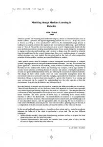
Fig. 1.1 Some AI pioneers AI.From top left to bottom right: Alan Turing, Arthur Lee Samuel, Marvin Minsky, Richard Bellman, Frank Rosenblatt, Geoffrey Hinton.

1.2

Stochastic modeling

In this course we discuss in some detail three different types of learning systems which are commonly categorized as supervised learning, unsupervised learning, and reinforcement learning. Supervised learning is characterized by given explicit examples that the system should learn (memorize) and from which the system should generalize to previously unseen examples. The supervision is usually given in the form of labels, y (i) for training patterns with features x(i) . This is usually contrasted with unsupervised learning, which aims to discover structure in data without explicit labels. Reinforcement learning is somewhat in between as the learning is guided only by some feedback on the quality of actions produced by the earning system rather than specifying what is right or wrong as can be done in supervised systems. We will also discuss hybrid systems. Traditional AI has provides many useful approaches for solving specific problems. For example, search algorithms can be used to navigate mazes or to find scheduling solutions, and such strategies should first be considered, However, learning systems are usually more general and can be applied to situations for which closed solutions are not be known. Also, experience has shown that applications often fail at some point since systems change over time or when an agent encounters situations for which the system has not been designed. Learning systems are generally thought to be more robust. Indeed, a main objective of learning systems is to build systems that generalize well to new situation, that is, learning systems should be able to generate sensible solutions to previously unseen situations. We will discuss this point in detail in Chapter 5.

Stochastic modeling

Another well known problem in building practical applications is that systems are generally unreliable and that environments are uncertain. For example, we a program might read data files in a specific format, but some users supplies a corrupted file. Productions software is often lengthy only to consider all kind of situations that could occur, and we now realize that considering all possibilities is often inpossible. This problem will become very apparent in robotics where sensors are often unreliable and estimation techniques are limited either because of limited resources or limited data. Even actions can be noisy. While the area of machine learning has a long history as outlined above, there has been major advances made over the last two decades. Much of the progress was made possible by the realization of researchers in many related areas that the language of (Bayesian) probability theory is very useful in this area. This language is appropriate since is acknowledges the fundamental limitations we have in real world applications (such as limited computational researches or inaccurate sensors). The language of probability theory has certainly helped to unify much of related areas and improved communication between researchers. Our aim of learning machines is to learn from the environment, either through instructions, by reward or punishment, or just by exploring the environment and learning about typical objects or temporal sequences. Our ultimate goal is to model the world and to use such models to make ‘smart’ decisions in order to maximize reward. The next two chapters are outlining some of the tools we will use to explore and describe this area. Chapter 2 is a brief introduction to the Matlab programming environment that we will mainly use in the following, Chapter 3 shows you how to use the Lego NXT and how to control them with Matlab. This chapter also includes a discussion of the important concept of a configuration space and how to plan movements with a robot arm. Chapter 4is a refresher on basic probability theory. The rest of the course is then divided into supervised, unsupervised, and reinforcement learning.

|5

2

Programming with Matlab

This chapter is a brief introduction to programming with the Matlab programming environment. We assumes thereby little programming experience, although programmers experienced in other programming languages might want to scan through this chapter. MATLAB is an interactive programming environment for scientific computing. This environment is very convenient for us for several reasons, including its interpreted execution mode, which allows fast and interactive program development, advanced graphic routines, which allow easy and versatile visualization of results, a large collection of predefined routines and algorithms, which makes it unnecessary to implement known algorithms from scratch, and the use of matrix notations, which allows a compact and efficient implementation of mathematical equations and machine learning algorithms. MATLAB stands for matrix laboratory, which emphasizes the fact that most operations are array or matrix oriented. Similar programming environments are provided by the open source systems called Scilab and Octave. The Octave system seems to emphasize syntactic compatibility with MATLAB, while Scilab is a fully fledged alternative to MATLAB with similar interactive tools. While the syntax and names of some routines in Scilab are sometimes slightly different, the distribution includes a converter for MATLAB programs. Also, the Matlab web page provides great videos to learn how to use Matlab at http://www.mathworks.com/demos/matlab/... ...getting-started-with-matlab-video-tutorial.html.

2.1

The MATLAB programming environment

MATLAB1 is a programming environment and collection of tools to write programs, execute them, and visualize results. MATLAB has to be installed on your computer to run the programs mentioned in the manuscript. It is commercially available for many computer systems, including Windows, Mac, and UNIX systems. The MATLAB web page includes a set of brief tutorial videos, also accessible from the demos link from the MATLAB desktop, which are highly recommended for learning MATLAB. As already mentioned, there are several reasons why MATLAB is easy to use and appropriate for our programming need. MATLAB is an interpreted language, which means that commands can be executed directly by an interpreter program. This makes the time-consuming compilation steps of other programming languages redundant and allows a more interactive working mode. A disadvantage of this operational mode is that the programs could be less efficient compared to compiled programs. However, there are two possible solution to this problem in case efficiency become a concern. The first is that the implementations of many MATLAB functions is very efficient 1 MATLAB and Simulink are registered trademarks, and MATLAB Compiler is a trademark of The MathWorks, Inc.


and are themselves pre-compiled. MATLAB functions, specifically when used on whole matrices, can therefore outperform less well-designed compiled code. It is thus recommended to use matrix notations instead of explicit component-wise operations whenever possible. A second possible solutions to increase the performance is to use the MATLAB compiler to either produce compiled MATLAB code in .mex files or to translate MATLAB programs into compilable language such as C. A further advantage of MATLAB is that the programming syntax supports matrix notations. This makes the code very compact and comparable to the mathematical notations used in the manuscript. MATLAB code is even useful as compact notation to describe algorithms, and it is hence useful to go through the MATLAB code in the manuscript even when not running the programs in the MATLAB environment. Furthermore, MATLAB has very powerful visualization routines, and the new versions of MATLAB include tools for documentation and publishing of codes and results. Finally, MATLAB includes implementations of many mathematical and scientific methods on which we can base our programs. For example, MATLAB includes many functions and algorithms for linear algebra and to solve systems of differential equations. Specialized collections of functions and algorithms, called a ‘toolbox’ in MATLAB, can be purchased in addition to the basic MATLAB package or imported from third parties, including many freely available programs and tools published by researchers. For example, the MATLAB Neural Network Toolbox incorporates functions for building and analysing standard neural networks. This toolbox covers many algorithms particularly suitable for connectionist modelling and neural network applications. A similar toolbox, called NETLAB, is freely available and contains many advanced machine learning methods. We will use some toolboxes later in this course, including the LIBSVM toolbox and the MATLAB NXT toolbox to program the Lego robots. 2.1.1

Starting a MATLAB session

Starting MATLAB opens the MATLAB desktop as shown in Fig. 2.1 for MATLAB version 7. The MATLAB desktop is comprised of several windows which can be customized or undocked (moving them into an own window). A list of these tools are available under the desktop menu, and includes tools such as the command window, editor, workspace, etc. We will use some of these tools later, but for now we only need the MATLAB command window. We can thus close the other windows if they are open (such as the launch pad or the current directory window); we can always get them back from the desktop menu. Alternatively, we can undock the command window by clicking the arrow button on the command window bar. An undocked command window is illustrated on the left in Fig. 2.2. Older versions of MATLAB start directly with a command window or simply with a MATLAB command prompt >> in a standard system window. The command window is our control centre for accessing the essential MATLAB functionalities. 2.1.2

Basic variables in MATLAB

The MATLAB programming environment is interactive in that all commands can be typed into the command window after the command prompt (see Fig. 2.2). The

|7

8 | Programming with Matlab

Fig. 2.1 The MATLAB desktop window of MATLAB Version 7.

Fig. 2.2 A MATLAB command window (left) and a MATLAB figure window (right) displaying the results of the function plot sin developed in the text.

commands are interpreted directly, and the result is returned to (and displayed in) the command window. For example, a variable is created and assigned a value with the = operator, such as >> a=3


a = 3 Ending a command with semicolon (;) suppresses the printing of the result on screen. It is therefore generally included in our programs unless we want to view some intermediate results. All text after a percentage sign (%) is not interpreted and thus treated as comment, >> b=’Hello World!’; % delete the semicolon to echo Hello World! This example also demonstrates that the type of a variable, such as being an integer, a real number, or a string, is determined by the values assigned to the elements. This is called dynamic typing. Thus, variables do not have to be declared as in some other programming languages. While dynamic typing is convenient, a disadvantage is that a mistyped variable name can not be detected by the compiler. Inspecting the list of created variables is thus a useful step for debugging. All the variables that are created by a program are kept in a buffer called workspace. These variable can be viewed with the command whos or displayed in the workspace window of the MATLAB desktop. For example, after declaring the variables above, the whos command results in the responds >> whos Name a b

Size

Bytes

1x1 1x12

8 24

Class

Attributes

double char

It displays the name, the size, and the type (class) of the variable. The size is often useful to check the orientation of matrices as we will see below. The variables in the workspace can be used as long as MATLAB is running and as long as it is not cleared with the command clear. The workspace can be saved with the command save filename, which creates a file filename.mat with internal MATLAB format. The saved workspace can be reloaded into MATLAB with the command load filename. The load command can also be used to import data in ASCII format. The workspace is very convenient as we can run a program within a MATLAB session and can then work interactively with the results, for example, to plot some of the generated data. Variables in MATLAB are generally matrices (or data arrays), which is very convenient for most of our purposes. Matrices include scalars (1 × 1 matrix) and vectors (1 × N matrix) as special cases. Values can be assigned to matrix elements in several ways. The most basic one is using square brackets and separating rows by a semicolon within the square brackets, for example (see Fig. 2.2), >> a=[1 2 3; 4 5 6; 7 8 9] a = 1 4 7

2 5 8

3 6 9

|9


A vector of elements with consecutive values can be assigned by column operators like >> v=0:2:4 v = 0

2

4

Furthermore, the MATLAB desktop includes an array editor, and data in ASCII files can be assigned to matrices when loaded into MATLAB. Also, MATLAB functions often return matrices which can be used to assign values to matrix elements. For example, a uniformly distributed random 3 × 3 matrix can be generated with the command >> b=rand(3) b = 0.9501 0.2311 0.6068

0.4860 0.8913 0.7621

0.4565 0.0185 0.8214

The multiplication of two matrices, following the matrix multiplication rules, can be done in MATLAB by typing >> c=a*b c = 3.2329 8.5973 13.9616

4.5549 10.9730 17.3911

2.9577 6.8468 10.7360

This is equivalent to c=zeros(3); for i=1:3 for j=1:3 for k=1:3 c(i,j)=c(i,j)+a(i,k)*b(k,j); end end end which is the common way of writing matrix multiplications in other programming languages. Formulating operations on whole matrices, rather than on the individual components separately, is not only more convenient and clear, but can enhance the programs performance considerably. Whenever possible, operations on whole matrices should be used. This is likely to be the major change in your programming style when converting from another programming language to MATLAB. The performance disadvantage of an interpreted language is often negligible when using operations on


whole matrices. The transpose operation of a matrix changes columns to rows. Thus, a row vector such as v can be changed to a column vector with the MATLAB transpose operator (’), >> v’ ans = 0 2 4 which can then be used in a matrix-vector multiplication like >> a*v’ ans = 16 34 52 The inconsistent operation a*v does produce an error, >> a*v ??? Error using ==> mtimes Inner matrix dimensions must agree. Component-wise operations in matrix multiplications (*), divisions (/) and potentiation ∧ are indicated with a dot modifier such as >> v.^2 ans = 0

4

16

The most common operators and basic programming constructs in MATLAB are similar to those in other programming languages and are listed in Table 2.1. 2.1.3

Control flow and conditional operations

Besides the assignments of values to variables, and the availability of basic data structures such as arrays, a programming language needs a few basic operations for building loops and for controlling the flow of a program with conditional statements (see Table 2.1). For example, the for loop can be used to create the elements of the vector v above, such as >> for i=1:3; v(i)=2*(i-1); end >> v v =

| 11

12 | Programming with Matlab Table 2.1 Basic programming contracts in MATLAB.

Programming construct

Command Syntax

Assignment Arithmetic operations

=

Logical

division power equal not equal less than AND

operators Loop

OR for

a=b a+b a*b (matrix), a.*b (element-wise) a/b (matrix), a./b (element-wise) a∧ b (matrix), a.∧ b (element-wise) a==b a∼=b a> for i=1:10; if i>4 & i> v2 v2 = 0

0

0

0

1

1

1

In this loop, the statement v2(i)=1 is only executed when the loop index is larger than 4 and less or equal to 7. Thus, when i=5, the array v2 with 5 elements is created, and since only the elements v2(5) is set to 1, the previous elements are set to 0 by default. The loop adds then the two element v2(6) and v2(7). Such a vector can also be created by assigning the values 1 to a specified range of indices, >> v3(4:7)=1 v3 =


0

0

0

1

1

1

1

A 1 × 7 array is thereby created with elements set to 0, and only the specified elements are overwritten with the new value 1. Another method to write compact loops in MATLAB is to use vectors as index specifiers. For example, another way to create a vector with values such as v2 or v3 is >> i=1:10 i = 1

2

3

4

5

6

7

0

1

1

1

8

9

10

>> v4(i>4 & i> hist(a) The result is shown in Fig. 2.4. This histogram shows that not all states are equally likely as we implicitly assumed in the above agent model. The third state is indeed much less likely. We could use this knowledge in a modified model in which we predict that the agent is sleeping for sensory states less than 1.5 and is eating otherwise. This modified model, which completely ignores study states, predicts around 65% of the states correctly. Many machine learning methods suffer from such ‘explaining away’ solutions for imbalanced data, as further discussed in Chapter ??. It is important to recognize that 100% accuracy is not achievable with the inherent limitations of the sensors. However, higher recognition rates could be achieved with better world (creature + sensor) models. The main question is how to find such a model. We certainly should use observed data in a better way. For example, we could use several observations to estimate how many states are produced by function creature state() and their relative frequency. Such parameter estimation is a basic form of learning from data. Many models in science take such an approach by proposing a parametric model and estimating parameters from the data by model fitting. The main challenge with this approach is how complex we should make the model. It is much easier to fit a more complex model with many parameters to example data, but the

| 17

Number of occurences in 1000 trials


Fig.

2.4 The

500 400 300 200 100 0 1

MATLAB desktop

1.5 2 2.5 Creature state value

window

histogram

3

of

states

produced

by

function

creature state() from 1000 trials. increased flexibility decreases the prediction ability of such models. Much progress has been made in machine learning by considering such questions, but those approaches only work well in limited worlds, certainly much more restricted than the world we live in. More powerful methods can be expected by learning how the brain solves such problems.

2.3

Alternative programming environments: Octave and Scilab

We briefly mention here two programming environments that are very similar to Matlab and that can, with certain restrictions, execute Matlab scripts. Both of these programming systems are open source environments and have general public licenses for non-commercial use. The programming environment called Octave is freely available under the GNU general public license. Octave is available through links at http://www.gnu.org/software/octave/. The installation requires the additional installation of a graphics package, such as gnuplot or Java graphics. Some distributions contain the SciTE editor which can be used in this environment. An example of the environment is shown in Fig. 2.5 Scilab is another scientific programming environment similar to MATLAB. This software package is freely available under the CeCILL software license, a license compatible to the GNU general public license. It is developed by the Scilab consortium, initiated by the French research centre INRIA. The Scilab package includes a MATLAB import facility that can be used to translate MATLAB programs to Scilab. A screen shot of the Scilab environment is shown in Fig. 2.6. A Scilab script can be run from the execute menu in the editor, or by calling exec("filename.sce").

2.4

Exercises

1. Write a Matlab function that takes a character string and prints out the character string in reverse order. reverses program 2. Write a Matlab program that plots a two dimensional gaussian function.

Exercises

Fig. 2.5 The Octave programming environment with the main console, and editor called SciTE, and a graphics window.

Fig. 2.6 The Scilab programming environment with console, and editor called SciPad, and a graphics window.

| 19

3

Basic robotics with Lego NXT

3.1

Introduction

"Robotics is the science of perceiving and manipulating the physical world through computer-controlled devices"2 . We use the word robot or agent to describe a system which interacts actively with the environment through sensors and actuators. An agent can be implemented in software or hardware, and we often use the term robot more specifically for a hardware implementation of an agent, though this does generally include software components. Active interactions means that the robot’s position in the environment or the environment itself changes though the action of the robot. Mobile robots are a good example of this and are mainly used in the examples of this course. In contrast, a vision system that uses a digital camera to recognize objects is not a robot in our definition. The word ‘robot’ was first used in print in a novel by Isaac Asimov (1941), and the first industrial robots were installed in 1961 (Unimate). Robots are now invaluable in manufacturing, and research is ongoing to make robots more autonomous and to make those machines more robust and able to work in hostile environments. Robotics has many components, including mechanical and electrical engineering, computer or machine vision, and even behavioral studies have become prominent in this field. In this course, we will demonstrate many of the discussions, algorithms and associated problems with the help of computer simulations and robots. Computer simulations are a great way to experiment with many of the ideas, but physical implementations have often the advantage to show more clearly the challenges in real applications. We will use the LEGO mindstorm system in this course. Besides having common LEGO building blocks to construct different designs, this system consist of a microprocessor, called the brick, which is programmable and which controls the sensors and actuators. The actuators are stepping motors that can be told to run for a specific duration, a specific number of rotations, or with a specific speed. Our tool kit also includes several sensors, a light sensor that can be used to measure the wavelength of reflecting light and also small distances, an ultrasonic sensor to measure larger distances, a touch sensor, and a microphone. The motors can also be used to sense some externally applied movements. We will use a basic tribot design as shown in Fig.3.1 for most of the explorations in this course. We will build the basic tribot in the following tutorial and will outline an example of a program to avoids walls and then work on a program so that the tribot can follow a line. After this we will use a robot arm configuration to discuss the important concept of a configuration space and demonstrate path-planing.

2 Probabilistic

Robotics, Sebastian Thrun, Wolfram Burgard, and Dieter Fox, MIT press 2006

Building a basic robot with Lego NXT

Fig. 3.1 Basic Lego Robot with microprocessor, two motors, and a light sensor.

3.2 3.2.1

Building a basic robot with Lego NXT Building the tribot

1. Charge the battery Before constructing the robot, plug the battery pack into the NXT brick controller and plug it into an outlet to recharge the battery.

2. Construct the NXT Follow the instruction booklet included with the Lego kit to construct the robot. There are mini programs illustrated in the manual that can be implemented directly on the NXT brick. Although this is not the method that will be used to control the NXT, you may implement them if you have time in order to get an idea of how the sensors and motors function. The instruction manual is organized as follows:

| 21

22 | Basic robotics with Lego NXT Section

3.2.2

Pages

NXT brick base construction

8-23

Sound sensor mounting Ultrasonic sensor mounting Light sensor mounting Touch sensor mounting

24-27 28-31 32-39 40-45

Mindstorm NXT toolbox instalation

We will use some software to control the Lego actuator and gather information from their sensors within the Matlab programming environment. To enable this we need to install software developed at the German university called ‘RWTH Aachen’, which in turn uses some other drivers that we need to install. Most of the software should be installed in our Lab, but we will outline briefly some of the installation issues in case you want to install them under your own system or if some problems exists with the current installation. The following software installation instructions are adapted from RWTH Aachen University’s NXT Toolbox website: http://www.mindstorms.rwth-aachen.de/trac/wiki/Download4.03 1. Check NXT Firmware version Check what version of NXT Firmware is running on the NXT brick by going to "Settings" > "NXT Version". Firmware version ("FW") should be 1.28. If it does not, it needs to be updated (Note: The NXT toolbox website claims version 1.26 will work, however it will not) To update the firmware: The Lego Mindstorms Education NXT Programming software is required to update the firmware. In the NXT Programming software, look under "tools" > "Update NXT Firmware" > "browse", select the firmware’s directory, click "download".

Building a basic robot with Lego NXT

2. Install USB (Fantom) Driver (Windows only) If the Lego Mindstorms Education NXT Programming software is already on your computer, this should already be installed. Otherwise, download it from: http://mindstorms.lego.com/support/updates/ If you run into problems with the Fantom Library on windows go to this site for help. http://bricxcc.sourceforge.net/NXTFantomDriverHelp.pdf If you have Windows 7 Starter edition the standard setup file will not run properly. To install the Fantom Driver go into Products and then LEGO NXT Driver 32 and run LegoMindstormsNXTdriver32. The fantom USB driver seem not to work on the Mac, but we will anyhow use the bluetooth connections. 3. Download the Mindstorms NXT Toolbox 4.03: Download: http://www.mindstorms.rwth-aachen.de/trac/wiki/Download • Save and extract the files anywhere, but do not change the directory structure. • The folder will appear as "RWTHMindstormsNXT" 4. Install NXT Toolbox into MATLAB In MATLAB: "File" > "SetPath" > "Add Folder", and browse and select "RWTHMindstormsNXT" - the file you saved in the previous step. • Also add the "tools" folder, which is a subdirectory of the RWTHMindstormsNXT folder. • Click "save" when finished. 5. Download MotorControl to NXT brick Go to http://bricxcc.sourceforge.net/utilities.html for the download. Use the USB cable for this step Windows: Download NeXTTool.exe to RWTHMindstormsNXT/tools/MotorControl. Under RWTHMindstormsNXT/tools/MotorControl, double click TransferMotorControlBinaryToNXT, click "Run", and follow the onscreen instructions. If this fails, try using the NBC compiler (download from http://bricxcc.sourceforge.net/nbc/) instead of the NeXTTool; again save it under the MotorControl folder. Mac: Download the NeXTTools for Mac OS X. Run the toolbar and open the XNT Explorer (the globe in the toolbar). With the arrow key at the top, transfer the file MotorControl21.rxe to the brick. 6. Setting up a Bluetooth connection To connect to the NXT via bluetooth you must first turn on the bluetooth in the NXT and make sure that the visibility is set to on. Then use the bluetooth device on your computer to search for your specific NXT. By default the name is NXT, but as a first step we will rename each brick. Create a connection between the computer and the NXT. When you create the connection between the NXT and the bluetooth device the NXT will ask for a passkey (usually either 0000 or 1234 on the NXT screen and press the orange

| 23

24 | Basic robotics with Lego NXT

button. The computer will then ask for the same passkey. To test the connection, type the command COM OpenNXT(’bluetooth.ini’); in the Matlab command window. The command should run without any red error messages. If there is an error check to see if the COMPort the Matlab code is looking for is the same as the one used in the connection made between the bluetooth device and the NXT. Also turning the NXT off and back on again can help. After every failed COM OpenNXT(’bluetooth.ini’); command type COM CloseNXT(’all’); to close the failed connection for a clean new attempt. To switch on a debug mode enter the command DebugMode on before entering the command COM OpenNXT(’bluetooth.ini’); . Also, make sure that the bluetooth.ini file is present. There are sample files for Windows ad Linux (Mac) in the main RWTH toolbox folder. Also, check if the port name is correct by typing ls -ltr /dev in a terminal window. 7. Does it work? In MATLAB, enter the commands below into the command window. The command should execute without error and the NXT should play a sound. h=COM OpenNXT(’bluetooth.ini’); COM SetDefaultNXT(h); NXT PlayTone(400,300);

A list of Matlab commands from the NXT toolbox can be found in Appendix A. Also, there are some examples included with the RWTH Mindstorm’s NXT Toolbox, under RWTHMindstormsNXT/demos.

First examples

3.3

| 25

First examples

The following exercises are intended to explore how to use RWTH’s Mindstorms NXT Toolbox. 3.3.1

Example 1: Wall avoidance

The following is a simple example of how to drive a robot and use the ultrasonic sensor. The robot will drive forward until it is around 20 cm away from a barrier (i.e. a wall), stop, beep, turn right, and continue moving forward. The robot will repeat this 5 times. Attach the Ultrasonic sensor and connect it to port 1. The study and run the following program. COM CloseNXT(’all’);

%cleans up workspace

close all; clear all; hNXT=COM OpenNXT(’bluetooth.ini’); COM SetDefaultNXT(hNXT);

% initiates NXT, hNXT is an arbitrary name %sets default handle

OpenUltrasonic(SENSOR 1); forward=NXTMotor(’BC’;); &% setting motors B C to drive forward forward.Power=50; forward.TachoLimit=0; turnRight=NXTMotor(’B’); &% setting motor B to turn right turnRight.Power=50; turnRight.TachoLimit=360; for i= 1:5 while GetUltrasonic(SENSOR 1)>20 forward.SendToNXT();

%sends command for robot to move forward %TachoLimit=0; no need for a WaitFor() statement

end %while forward.Stop(’brake’); NXT PlayTone(400,300); turnRight.SendToNXT; turnRight.WaitFor; end %for turnRight.Stop(’off’); forward.Stop(’off’); CloseSensor(SENSOR 1); COM CloseNXT(hNXT); close all; clear all;

3.3.2

%robot brakes from going forward %plays a note %sends the command to turn right %TachoLimit is not 0; WaitFor() statement required %properly closes motors %properly closes the sensor % properly closes the NXT

Example 2: Line following

The next exercise is writing your own program that uses readings from its light sensor to drive the NXT and follow a line.


Setup: 1. Mount light sensor, facing downwards on front of NXT and plugged into Port 3. 2. Mount a switch sensor on the NXT, plugged into Port 2. 3. Use a piece of dark tape (i.e. electrical tape) to mark a track on a flat, light coloured surface. Make sure the tape and the surface are coloured differently enough that the light sensor returns reasonably different values between the two surfaces. 4. Write a program so that the tibot follows the line.

3.4 3.4.1

Configuration space Abstracting the states of a system

Very important for most algorithms to control a robot is the description of its state or the possible states of the system. The physical state of an agent can be quite complicated. For example, the Lego components of the tribot can have different positions and can shift in operation; the battery will have different levels of charge during the day, lightening conditions change, etc. Thus, description of the physical state would need a lot of variables, and such a description space would be very high dimensional, which is one important source of the computational challenges we face. To manage this problem we need to consider abstractions. Abstraction is an important concept in computer science and science in general. To abstract means to simplify the system in a way that it can be described in as simple terms as possible to answer the specific questions under consoderation. This philosophy is sometimes called the principle of parsimony, also known as Occam’s razor. Basically, we want a model as simple as possible, while still capturing the main aspects of the system that the model should capture. For example, let us consider a robot that should navigate around some obstacles from point A to point B as shown in Fig.3.2A. The simplifications we make in the following is that we take consider the movement in only in a two-dimensional (2D) plane. The robot will have a position described by an x and y coordinate, and a heading direction described by an angle α. Note that we ignore for now the physical extension of the robot, that is, we consider it here only as a point object. If this is a problem, we can add an extension parameter later. We also ignore many of the other physical

Configuration space

parameters mention above. The current state of robot is hence described by three real numbers, [x, y, α], and the space of all possible values is called the configuration space or state space. An obstacle, as shown in Fig.3.2A with the grey area, can be represented as state values that are not allowed by the system. A. Navigation with obstracle

B. Discrete configuration space

A

A

B

B

Fig. 3.2 (A) A physical space with obstacles in which an agent should navigate from point point B . (B) Descretized configuration space.

A to

We have reduced the description of an robot navigation system from a nearly infinite physical space to a three-dimensional (3D) configuration space by the process of abstraction. However, there are still an infinite number of possible states in the state space if the state variables are real numbers. We will shortly see that we have often to search the state space, and an infinite space then often becomes problematic. A common solution to this problem is to make further abstractions and to allow the state variables to have only a finite number of states. Thus, we commonly discretize the state space. An example is shown in Fig.3.2B, where we used a grid to represent the possible values of the robot positions. Such a discretization is very useful in practice, and we can also make the discretization error increasingly small by decreasing the grid parameter, ∆x, which describes the minimal distance between two states. We will use this grid discretization for planing a path through the configuration space later in this chapter. 3.4.2

Robot Arm State Space Visualizer

The goal of the following exercise is to graph the state space in which a double jointed robot arm is able to move. To do this, use two motors of the NXT Lego kit as joins of this arm, similarly to the one pictured in Fig.3.3. Also attach a touch sensor that we will use as a button in the following. Secure it on the table so that you can move its pointing finger around by turning the externally moving the motors. We will use the ability of measuring this movement in the motors by the Lego system. Also, use a box, a coffee mug or some other items to create some obstacles for the arm to move around. Use the Matlab program in Table 3.1 to visualize the state space. Start the Matlab program with the robot arm touching one of the obstacles. Then move the arm all around one of the obstacles. This will allow the NXT to create set of data that will display which combinations of angles cannot be travelled through by the robot arm. To map more than one obstacle without mapping the angles in between the two obstacles, push the button. The button pauses the program for 4 seconds so that you can move

| 27


Fig. 3.3 (A) Robot arm with two joints. (B)

the arm from one obstacle to the next without mapping the angles in between the two. 3.4.3

Exercise

1. Write a program that produces a map of the state space in form of a matrix which has zeros of entries that can be reached and ones as entries for states that have obstacles in it.

3.5

Planning

Planing a movement is basic requirement in robotics. In particular, we want to find the shortest path from a starting position to a goal position. The previous exercise provides us with a map that we can use to plan the movement. One of the elements of the array is dedicated as the starting position, and one as the goal position. We now need to write a search algorithm that finds the shortest path. There are many search algorithms that we could utilize for this task. For example, a basic search algorithm is depth-first-search that choses a neighboring node, than

Planning Table 3.1 State space visualization program

for counter = 1:10000 %The angles for both wheels are read bottomDeg=bottom.ReadFromNXT.Position; topDeg=top.ReadFromNXT.Position; %the angles are then stored in angleWheel angleWheel(1,counter)=bottomDeg; angleWheel(2,counter)=topDeg; %This plot will show all the angles read from the %wheels, because hold is on plot(topDeg,bottomDeg,’o’); %If the switch is pushed then pause the angle reader if GetSwitch(SENSOR_1)==1 disp(’paused’); pause(4); disp(’unpaused’); end end

moves to the next, etc, until it reaches a goal. If the algorithm ends up in a dead-end, than the algorithm tracks back to the last node with another options and goes down this node. The breadth-first-search algorithms searches instead first if each of the neighboring nodes of a current node is the goal state before advancing to the next level. Of course, both need to keep track of which routs have been tried already to ensure that we do not continuously try failed paths. These algorithms would sooner or later find a path between the starting position and the goal if it exists since these algorithms would try out all possible paths. However, these algorithms do not grantee to find the shortest path, and these algorithms are also usually not so efficient. To find better solutions we could take more information into account. For example, in the grid world, we can use some distance measure between the current state and the goal, such as the Euclidean distance g(current) =

q

(xgoal − xcurrent )2 + (ygoal − ycurrent )2 ,

(3.1)

to guide the search3 . That is, if we chose the next node to expand, we would chose the node that has the smallest distance to the goal node. Such a heuristic search algorithm is sometimes called a gready best-first search. Valid heuristics, which are estimations of the expected cost that must not underestimate the real cost, can greatly accelerate search performance. We can take such strategy a step further by also taken into account in the cost of reaching the current state from the starting state, h(current) =

p

(xstart − xcurrent )2 + (ystart − ycurrent )2 ,

(3.2)

3 This distance measure is also called the L norm. Other measures such as the Manhattan distance, the 2 Minkowski distance, or the L1 norm also frequently used.

| 29


so that the total heuristic cost of node ‘current’ is f (current) = h(current) + g(current).

(3.3)

The algorithm that uses this heuristics while taking track of paths that are still ‘open’ or that are ‘closed’ since they lead to dead-ends, is called an A∗ star search algorithm. An Matlab example and visualization of the A∗ search algorithm is provided on the course web page. 3.5.1

Exercise: Robot Arm State Space Traversal

The goal of this exercise is to make the double jointed NXT arm progress through the state space. You need the double-joined robot arm and the obstacles from the state space visualization exercise above. • Make a program which can move the arm from the starting coordinate to the ending coordinate while avoiding the obstacles in the state space.

4

Basic probability theory

As outlined in Chapter 1, a major milestone for the modern approach to machine learning is to acknowledge our limited knowledge about the world and the unreliability of sensors and actuators. It is then only natural to consider quantities in our approaches as random variables. While a regular variable, once set, has only one specific value, a random variable will have different values every time we ‘look’ at it (draw an example from the distributions). Just think about a light sensor. We might think that an ideal light sensor will give us only one reading while holding it to a specific surface, but since the peripheral light conditions change, the characteristics of the internal electronic might change due to changing temperatures, or since we move the sensor unintentionally away from the surface, it is more than likely that we get different readings over time. Therefore, even internal variables that have to be estimated from sensors, such as the state of the system, is fundamentally a random variable. Having a random variable does not mean that we can not say anything about the variable. Some numbers might be more likely than others when applying the sensor. This knowledge, how likely each value is for a random variable x, is captured by the probability density function pdf (x). Most of the systems discussed in this course are stochastic models to capture the uncertainties in the world. Stochastic models are models with random variables, and it is therefore useful to remind ourselves about the properties of such variables. This chapter is a refresher on concepts in probability theory. Note that we are mainly interested in the language of probability theory rather than statistics, which is more concerned with hypothesis testing and related procedures.

4.1

Random numbers and their probability (density) function

Probability theory is the theory of random numbers. We denoted such numbers by capital letters to distinguish them from regular numbers written in lower case. A random variable, X, is a quantity that can have different values each time the variable is inspected, such as in measurements in experiments. This is fundamentally different to a regular variable, x, which does not change its value once it is assigned. A random number is thus a new mathematical concept, not included in the regular mathematics of numbers. A specific value of a random number is still meaningful as it might influence specific processes in a deterministic way. However, since a random number can change every time it is inspected, it is also useful to describe more general properties when drawing examples many times. The frequency with which numbers can occur is then the most useful quantity to take into account. This frequency is captured by the mathematical construct of a probability.

32 | Basic probability theory

We can formalize this with some compact notations. We speak of a discrete random variable in the case of discrete numbers for the possible values of a random number. A continuous random variable is a random variable that has possible values in a continuous set of numbers. There is, in principle, not much difference between these two kinds of random variables, except that the mathematical formulation has to be slightly different to be mathematically correct. For example, the probability function, PX (x) = P (X = x)

(4.1)

describes the frequency with which each possible value x of a discrete variable X occurs. Note that x is a regular variable, not a random variable. The value of PX (x) gives the fraction of the times we get a value x for the random variable X if we draw many examples of the random variable.4 From this definition it follows that the frequency of having any of the possible values is equal to one, which is the normalization condition X PX (x) = 1. (4.2) x

In the case of continuous random numbers we have an infinite number of possible values x so that the fraction for each number becomes infinitesimally small. It is then appropriate to write the probability distribution function as PX (x) = pX (x)dx, where pX (x) is the probability density function (pdf). The sum in eqn 4.2 then becomes an integral, and normalization condition for a continuous random variable is Z pX (x)dx = 1.

(4.3)

x

We will formulate the rest of this section in terms of continuous random variables. The corresponding formulas for discrete random variables can easily be deduced by replacing the integrals over the pdf with sums over the probability function. It is also possible to use the δ-function, outlined in Appendix ??, to write discrete random processes in a continuous form.

4.2

Moments: mean, variance, etc.

In the following we only consider independent random values that are drawn from identical pdfs, often labeled as iid (independent and identically distributed) data. That is, we do not consider cases where there is a different probabilities of getting certain numbers when having a specific number in a previous trial. The static probability density function describes, then, all we can know about the corresponding random variable. Let us consider the arbitrary pdf, pX (x), with the following graph:

4 Probabilities

are sometimes written as a percentage, but we will stick to the fractional notation.

Moments: mean, variance, etc.

p(x)

µ

x

Such a distribution is called multimodal because it has several peaks. Since this is a pdf, the area under this curve must be equal to one, as stated in eqn 4.3. It would be useful to have this function parameterized in an analytical format. Most pdfs have to be approximated from experiments, and a common method is then to fit a function to the data. However, sometimes it is sufficient to know at least some basic characteristics of the functions. For example, we might ask what the most frequent value is when drawing many examples. This number is given by the largest peak value of the distribution. A more common quantity to know is the expected arithmetic average of those numbers, which is called the mean, expected value, or expectation value of the distribution, defined by Z ∞

µ=

xf (x)dx.

(4.4)

−∞

In the discrete case, this formula corresponds to the formula of calculating an arithmetic average, where we add up all the different numbers together with their frequency. Formally, we need to distinguish between a quantity calculated from random numbers and quantities calculated from the pdfs. If we treat the pdf as fundamental, then the arithmetic average is like an estimation of the mean. This is usually how it is viewed. However, we could also be pragmatic and say that we only have a collection of measurements so that the numbers are the ‘real’ thing, and that pdfs are only a mathematical construct. While this is mainly a philosophical debate, we try to be consistent in calling the quantities derived from data ‘estimates’ of the quantities defined through pdfs. The mean of a distribution is not the only interesting quantity that characterizes a distribution. For example, we might want to ask what the median value is for which it is equally likely to find a value lower or larger than this value. Furthermore, the spread of the pdf around the mean is also very revealing as it gives us a sense of how spread the values are. This spread is often characterized by the standard deviation (std), or its square, which is called variance, σ 2 , and is defined as Z ∞ σ2 = (x − µ)2 f (x)dx. (4.5) −∞

This quantity is generally not enough to characterize the probability function uniquely; this is only possible if we know all moments of a distribution, where the nth moment about the mean is defined as Z ∞ mn = (x − µ)n f (x)dx. (4.6) −∞

| 33


The variance is the second moment about the mean, Z ∞ σ2 = (x − µ)2 f (x)dx.

(4.7)

−∞

Higher moments specify further characteristics such as the kurtosis and skewness of the distribution. Moments higher than this have not been given explicit names. Knowing all moments of a distribution is equivalent in knowing the distribution precisely, and knowing a pdf is equivalent in knowing everything we could know about a random variable. In case the distribution function is not given, moments have to be estimated from data. For example, the mean can be estimated from a sample of measurements by the sample mean, n 1X xi , (4.8) x ¯= n i=1 and the variance either from the biased sample variance, n

s21 =

1X (¯ x − xi )2 , n i=1

(4.9)

or the unbiased sample variance n

s22 =

1 X (¯ x − xi )2 . n − 1 i=1

(4.10)

A statistic is said to be biased if the mean of the sampling distribution is not equal to the parameter that is intended to be estimated. Knowing all moments uniquely specifies a pdf.

4.3

Examples of probability (density) functions

There is an infinite number of possible pdfs. However, some specific forms have been very useful for describing some specific processes and have thus been given names. The following is a list of examples with some discrete and several continuous distributions. Most examples are discussed as one-dimensional distributions except the last example, which is a higher dimensional distribution. 4.3.1

Bernoulli distribution

A Bernoulli random variable is a variable from an experiment that has two possible outcomes: success with probability p; or failure, with probability (1 − p). Probability function: P (success) = p; P (failure) = 1 − p mean: p variance: p(1 − p)

Examples of probability (density) functions

4.3.2

Multinomial distribution

This is the distribution of outcomes in n trials that have k possible outcomes. The probability of each outcome is thereby pi . Probability function: Qk P (xi ) = n! i=1 (pxi i /xi !) mean: npi variance: npi (1 − pi ) An important example is the Binomial distribution (k = 2), which describes the the number of successes in n Bernoulli trials with probability of success p. Note that the binomial coefficient is defined as n! n = (4.11) x x!(n − x)! and is given by the MATLAB function nchoosek. P(x)

x

np

4.3.3

Probability function: n P (x) = px (1 − p)n−x x mean: np variance: np(1 − p)

Uniform distribution

Equally distributed random numbers in the interval a ≤ x ≤ b. Pseudo-random variables with this distribution are often generated by routines in many programming languages. p(x)

Probability density function: 1 p(x) = b−a mean: (a + b)/2 variance: (b − a)2 /12 x

4.3.4

Normal (Gaussian) distribution

Limit of the binomial distribution for a large number of trials. Depends on two parameters, the mean µ and the standard deviation σ. The importance of the normal distribution stems from the central limit theorem outlined below. p(x)

Probability density function: σ

p(x) = σ√12π e mean: µ variance: σ 2 µ

x

−(x−µ)2 2σ 2

| 35


4.3.5

Chi-square distribution

The sum of the squares of normally distributed random numbers is chi-square distributed and depends on a parameter ν that is equal to the mean. Γ is the gamma function included in MATLAB as gamma. p(x)

Probability density function: (ν−2)/2 −x/2 e p(x) = x 2ν/2 Γ(ν/2) mean: ν variance: 2ν ν

4.3.6

x

Multivariate Gaussian distribution

We will later consider density functions of a several random variables, x1 , ..., xn . Such density functions are functions in higher dimensions. An important example is the multivariate Gaussian (or Normal) distribution given by 1 1 p p(x1 , ..., xn ) = p(x) = p exp(− (x − µ)T Σ−1 (x − µ)). n 2 ( (2π)) ( det(Σ) (4.12) This is a straight forward generalization of the one-dimensional Gaussian distribution mentioned before where the mean is now a vector, µ and the variance generalizes to a covariance matrix, Σ = [Cov[Xi , Xj ]]i=1,2,...,k;j=1,2,...,k which must be symmetric and positive semi-definit. An example with mean µ = (1 2)T and covariance Σ = (1 0.5; 0.5 1 is shown in Fig,4.1.

4.4

Cumulative probability (density) function and the Gaussian error function

The probability of having a value x for the random variable X in the range of x1 ≤ x ≤ x2 is given by Z x2

P (x1 ≤ X ≤ x2 ) =

p(x)dx.

(4.13)

x1

Note that we have shortened the notation by replacing the notation PX (x1 ≤ X ≤ x2 ) by P (x1 ≤ X ≤ x2 ) to simplify the following expressions. In the main text we often need to calculate the probability that a normally (or Gaussian) distributed variable has values between x1 = 0 and x2 = y. The probability of eqn 4.13 then becomes a function of y. This defines the Gaussian error function Z y (x−µ)2 1 1 y−µ √ e− 2σ2 dx = erf( √ ). (4.14) 2 2πσ 0 2σ This Gaussian error function (erf) for normally distributed variables (Gaussian distribution with mean µ = 0 and variance σ = 1) is commonly tabulated in books on statistics. Programming libraries also frequently include routines that return the values

Cumulative probability (density) function and the Gaussian error function

4

3

2

1

0

−1

−2 −2

−1

0

Fig. 4.1 Multivariate Gaussian with mean µ

1

2

3

4

= (1 2)T and covariance Σ = (1 0.5; 0.5 1).

for specific arguments. In MATLAB this is implemented by the routine erf, and values for the inverse of the error function are returned by the routine erfinv. Another special case of eqn 4.13 is when x1 in the equation is equal to the lowest possible value of the random variable (usually −∞). The integral in eqn 4.13 then corresponds to the probability that a random variable has a value smaller than a certain value, say y. This function of y is called the cumulative density function (cdf),5 Z y cum p(x)dx, (4.15) P (x < y) = −∞ 5 Note

that this is a probability function, not a density function.

| 37


which we will utilize further below.

4.5

Functions of random variables and the central limit theorem

A function of a random variable X, Y = f (X),

(4.16)

is also a random variable, Y , and we often need to know what the pdf of this new random variable is. Calculating with functions of random variables is a bit different to regular functions and some care has be given in such situations. Let us illustrate how to do this with an example. Say we have an equally distributed random variable X as commonly approximated with pseudo-random number generators on a computer. The probability density function of this variable is given by 1 for 0 ≤ x ≤ 1, pX (x) = (4.17) 0 otherwise. We are seeking the probability density function pY (y) of the random variable 2

Y = e−X .

(4.18)

The random number Y is not Gaussian distributed as we might think naively. To calculate the probability density function we can employ the cumulative density function eqn 4.15 by noting that p 2 (4.19) P (Y ≤ y) = P (e−X ≤ y) = P (X ≥ − ln y). Thus, the cumulative probability function of Y can be calculated from the cumulative probability function of X, (R √ 1 p √ p (x)dy = 1 − − ln y for e−1 ≤ y ≤ 1, − ln y X P (X ≥ − ln y) = 0 otherwise. (4.20) The probability density function of Y is the the derivative of this function, √ 1 − − ln y for e−1 ≤ y ≤ 1, pY (y) = (4.21) 0 otherwise. The probability density functions of X and Y are shown below. 4

Y=e -X

0.5 0 -0.5

3

2

pY (y)

pX (x)

1

2 1 0

0

0.5

x

1

1.5

0

0.5

y

1

Measuring the difference between distributions

A special function of random variables, which is of particular interest it can approximate many processes in nature, is the sum of many random variables. For example, such a sum occurs if we calculate averages from measured quantities, that is, n

X ¯= 1 X Xi , n i=1

(4.22)

and we are interested in the probability density function of such random variables. This function depends, of course, on the specific density function of the random variables Xi . However, there is an important observation summarized in the central limit theorem. This theorem states that the average (normalized sum) of n random variables that are drawn from any distribution with mean µ and variance σ is approximately normally distributed with mean µ and variance σ/n for a sufficiently large sample size n. The approximation is, in practice, often very good also for small sample sizes. For example, the normalized sum of only seven uniformly distributed pseudo-random numbers is often used as a pseudo-random number for a normal distribution.

4.6

Measuring the difference between distributions

An important practical consideration is how to measure the similarity of difference between two density functions, say the density function p and the density function q. Note that such a measure is a matter of definition, similar to distance measures of real numbers or functions. However, a proper distance measure, d, should be zero if the items to be compared, a and b, are the same, itÕs value should be positive otherwise, and a distance measure should be symmetrical, meaning that d(a, b) = d(b, a). The following popular measure of similarity between two density functions is not symmetric and is hence not called a distance. It is called Kulbach–Leibler divergence and is given by dKL (p, q) =

Z p(x) log(

p(x) )dx q(x)

Z =

(4.23) Z

p(x) log(p(x))dx −

p(x) log(q(x))dx

(4.24)

This measure is zero if p = q since log(1) = 0. This measure is related to the information gain or relative entropy in information theory.

4.7

Density functions of multiple random variables

So far, we have discussed mainly probability (density) functions of single random variables. In many applications, we consider multiple random variables and their interactions, and some basic rules will be very useful. We start by illustrating these with two random variables and mention some generalizations at the end.

| 39


We have seen that probability theory is quite handy to model data, and probability theory also considers multiple random variables. The total knowledge about the cooccurance of specific values for two random variables X and Y is captured by the joined distribution: p(x, y) = p(X = x, Y = y).

(4.25)

This is a two dimensional functions. The two dimensions refers here to the number of variables, although a plot of this function would be a three dimensional plot. An example is shown in Fig.4.2. All the information we can have about a stochastic system is encapsulated in the joined pdf. The slice of this function, given the value of one variable, say y, is the conditional distribution: p(x|y) = p(X = x|Y = y).

(4.26)

A conditional pdf is also illustrated in Fig.4.2 If we sum over all realizations of y we get the Z marginal distribution: p(x) =

p(Y|X=0.4)

p(x, y)dy.

(4.27)

8 7 6 5 4 3 2 1

p(X,Y)

0

15

0

5

10

15

20

25

30

35

40

45

5

10

50

10 5

p(X|Y=0.88)

0 2

14

2

1

1

0

X

0 -1

-1 -2

-2

12 10 8 6

Y

4 2 0

0

15

20

25

30

35

p(X,Y)

Fig. 4.2 Example of a two-dimensional probability density function (pdf) and some examples of conditional pdfs.

If we know some functional form of the density function or have a parameterized hypothesis of this function, than we can use common statistical methods, such as maximum likelihood estimation, to estimate the parameters as in the one dimensional cases. If we do not have a parameterized hypothesis we need to use other methods, such as treating the problem as discrete and building histograms, to describe the density function of the system. Note that parameter-free estimation is more challenging with increasing dimensions. Considering a simple histogram method to estimate the joined density function where we discretize the space along every dimension into n bins.

40

45

50

Density functions of multiple random variables

This leads to n2 bins for a two-dimensional histogram, and nd for a d-dimensional problem. This exponential scaling is a major challenge in practice since we need also considerable data in each bin to sufficiently estimate the probability of each bin. As mentioned before, if we know the joined distribution of some random variables we can make the most predictions of these variables. However, in practice we have often to estimate these functions, and we can often only estimate conditional density functions. A very useful rule to know is therefore how a joined distribution can be decompose into the product of a conditional and a marginal distribution, p(x, y) = p(x|y)p(y) = p(y|x)p(x),

(4.28)

which is sometimes called the chain rule. Note the two different ways in which we can decompose the joined distribution. This is easily generalized to n random variables by p(x1 , x2 , ..., xn ) = p(xn |x1 , ...xn−1 )p(x1 , ..., xn−1 ) = p(xn |x1 , ..., xn−1 ) ∗ ... ∗ p(x2 |x1 ) ∗ p(x1 ) =

Πni=1 p(xi |xi−1 , ...x1 )

(4.29) (4.30) (4.31)

but note that there are also different decompositions possible. We will learn more about this and useful graphical representations in Chapter ??. If we divide this chain rule eq. 4.28 by p(x), which is possible as long as p(x) > 0, we get the identity p(y|x)p(x) , (4.32) p(x|y) = p(y) which is called Bayes theorem. This theorem is important because it tells us how to combine a prior knowledge, such as the expected distribution over a random variable such as the state of a system, p(x), with some evidence called the likelihood function p(y|x), for example by measuring some sensors reading y when controlling the state, to get the posterior distribution, p(y|x) from which the new estimation of state can be derived. The marginal distribution p(y), which does not depend on the state X, is the proper normalization so that the left-hand side is again a probability. Estimations of processes are greatly simplified when random variables are independent. A random variable X is independent of Y if p(x|y) = p(x).

(4.33)

Using the chain rule eq.4.28, we can write this also as p(x, y) = p(x)p(y),

(4.34)

that is, the joined distribution of two independent random variables is the product of their marginal distributions. Similar, we can also define conditional independence. For example, two random variables X and Y are conditionally independent of random variable Z if p(x, y|z) = p(x|z)p(y|z). (4.35) Note that total independence does not imply conditionally independence and visa versa, although this might hold true for some specific examples.

| 41


Exercises 1. Measure the response function of the light sensor and the ultrasonic sensor with regards to distance. How do the measurements vary in repeated measurments. Discuss briefly your experimental setup and results. 2. Write a Matlab program that produces and bimodal distributed (pseudo-)random variable. Plot a normalized histogram together with an indication of the mean, the median, and the variance. Plot the cumulative distribution for this random variable. 3. (From Thrun, Burgard and Fox, Probabilistic Robotics) A robot uses a sensor that can measure ranges from 0m to 3m. For simplicity, assume that the actual ranges are distributed uniformly in this interval. Unfortunately, the sensors can be faulty. When the sensor is faulty it constantly outputs a range below 1m, regardless of the actual range in the sensor’s measurement cone. We know that the prior probability for a sensor to be faulty is p = 0.01. Suppose the robot queries its sensors N times, and every single time the measurement value is below 1m. What is the posterior probability of a sensor fault, for N = 1, 2, ..., 10. Formulate the corresponding probabilistic model.

Part II Supervised learning

5

Regression, classification and maximum likelihood

This chapter start the discussion of an important subset of learning problems, that of supervised learning with labeled data. We start by considering regression with noisy data and formalize our learning objectives. This chapter includes some discussion of fundamental and important algorithms to solve the learning problem as minimization procedure.

5.1

Regression of noisy data

An important type of learning is supervised learning. In supervised learning, examples of input-output relations are given, and the goal is to learn the underlying mapping so that accurate predictions can be made for previously unseen data. For example, let us consider health records of 30 employees who were regular members of a company’s health club6 . We want to know the relation between the weight of the persons and their time in a one-mile run. These data are partially shown in a table in Fig.5.1 on plotted on the right of this figure with the Matlab commands load healthData; plot(x,y,’*’). The full data set is provided in file healthData.mat. time of one−mile run (seconds)

500 450 400 350 300 250 100

150

200 weight (pounds)

Fig. 5.1 Health data. 6 Source: Chatterjee, S. and Hadi, A.S. (1988). Sensitivity Analysis in Linear Regression. John Wiley & Sons: New York.

250

300

46 | Regression, classification and maximum likelihood

Looking at the plot reveals that there seems to be a systematic relation between the weights and running times, with a trend that heavier persons tend to be slower in the runs, although this is not true for all individuals. Moreover, the trend seems linear. This hypothesis can be quantified as a parameterized function, h(x; θ) = θ0 + θ1 x.

(5.1)

This notation means that the hypothesis h is a function of the quantity x, and the hypothesis includes all possible straight lines, where each line can have a different offset θ0 (intercept with the y-axis), and slope θ1 . We typically collect parameters in a parameter vector θ. We only considered on input variable x above, but we can easily generalize this to higher dimensional problems where more input attributes are given. For example, there might be the amount of exercise each week that might impact the results of running times. If we make the hypothesis that this additional variable has also a linear influence on the running time, independently of the other attribute, we can write the hypothesis as h(x; θ) = θ0 + θ1 x1 + θ2 x2 .

(5.2)

A useful trick to enable a compact notation in higher dimensions with n attributes is to introduce x0 = 1. We can then write the linear equations as X h(x; θ) = θ0 x0 + .... + θn xn = θi xi = θT x. (5.3) i

The vector θT is the transpose of the vector θ. In the following we consider m training examples, the pairs of values {(x(i) , y (i) ); i = 1...m},

(5.4)

which is also called a training set. We use here again an index counter i, though this is different than the index over the attributes used before. To distinguish this better, we write the index of training examples as superscript and use brackets around it to distinguish it from a potentiation operation. We can use the training examples to come-up with some reasonable values for the parameters. For example, a common technique is called least-mean-square (LMS) linear regression to determine those parameters. In this technique we chose values for θ that will minimize the sum of the mean square error (MSE) from the line to each data point. In general we consider a cost function to be minimized, which is in this case the square function 1 (y − h(x; θ))2 2 1 X (i) ≈ (y − h(x(i) ; θ))2 . 2m i

E(θ) =

(5.5) (5.6)

Note that the objective function is a function of the parameters. Also, there is a small subtlety in the above equation since we wrote the general form of the objective function in line 5.5 and considered its approximation with the data, considered to be independent,

Gradient Descent

in line 5.6. With this objective function, we reduced the learning problem to a search problem of finding the parameter values that minimize this objective function, θ = arg min E(θ) θ

(5.7)

We will demonstrate practical solutions to this search problem with three important methods. The first method is an analytical one. You might remember from basic mathematics classes that finding a minimum of a function f (x) is characterized by d2 f df dx = 0, and dx2 > 0. Here we have a vector function since the cost function depends an several parameters. The derivative then becomes a gradient 

∂E ∂θ0



 .     ∇θ E(θ) =   . .  . 

(5.8)

∂E ∂θn

It is useful to collect the training data in a large matrix for the x values, and a vector for the y values,  (1)T   (1)T  y x  .   .        (5.9) Y = X=  . .  .   .   .  y (m)T x(m)T We can then write the cost function in as E(θ) =

1 (Y − Xθ)T (Y − Xθ), 2m

(5.10)

The parameters for which the gradient is zero is then given by the normal equation θ = (X T X)−1 X T Y.

(5.11)

We have still to make sure these parameters are the minimum and and a maximum value, but this can easily be done and is also obvious when plotting the result. A second method we want to consider is random search. This is a very simple algorithm, but worthwhile considering to compare them to the other solutions. In this algorithm, a new random values for the parameters are tried, and these new parameters replace the old ones if the new values result in a smaller error value (see Matlab code in Tab.5.2).

5.2

Gradient Descent

The last method discussed here for finding a minimum for LMS regression is Gradient Descent. This method will often be used in the following and it will thus be reviewed here in more detail.

| 47

48 | Regression, classification and maximum likelihood Table 5.1 Program randomSearch.m

%% Linear regression with random search clear; clf; hold on; load healthData; E=1000000; for trial=1:100 thetaNew=[100*rand()+50, 3*rand()]; Enew=0.5*sum((y-(thetaNew(1)+thetaNew(2)*x)).^2); if Enew γ) ≤ 2 exp(−2γ 2 m). P (|R(hi ) − R(h

(8.37)

This formula states that there is a certain probability that we make an error larger than γ for each hypothesis of the empirical risk compared to the expected risk, although the good news is that this probability is bounded and that the bound itself becomes exponentially smaller with the number of validation examples. This is already an interesting results, but we now want to know the probability that some, out of all possible hypothesis, are less than γ. Using the fact that the probability of the union of several events is always less or equal to the sum of the probabilities, one can show that with probability 1 − δ the error of a hypothesis is bounded by r 2k 1 ˆ log . (8.38) |R(h) − R(h)| ≤ 2m δ This is a great results since it shows how the error of using an estimate the risk, the empirical risk that we can evaluate from the validation data, is getting smaller with training examples and with the number of possible hypothesis.

x x x

Fig. 8.5 Illustration of VC dimensions for the class of linear functions in two dimensions.

While the error scales only with the log of the number of possible hypothesis, the values goes still to infinite when the number of possible hypothesis goes to infinite, which much more resembles the situation when we have parameterized hypothesis. However, Vapnik was able to show the following generalization in the infinite case, which is that given a hypothesis space with Vapnic-Chervonencis dimension VC({h}),

| 83

84 | General learning machines

then, with probability 1 − δ, the error of the empirical risk compared to the expected risk (true generalization error) is ! r V C m 1 1 ˆ |R(h) − R(h)| ≤O log + log . (8.39) m VC m δ The VC dimensions is thereby a measure of how many points can be divided by a member of the hypothesis set for all possible label combinations of the point. For example, consider three arbitrary points in two dimensions as shown in figure 8.5, and let us consider the hypothesis class of all possible lines in two dimensions. I can always divide the three points under any class membership condition, of which two examples are also shown in the figure. In contrast, it is possible to easily find examples with four points that can not be divided by a line in two dimensions. The VC dimension of lines in two dimensions is hence V C = 3.11

8.3 8.3.1

SV-Regression and implementation Support Vector Regression

While we have mainly discussed classification in the last few sections, it is time to consider the more general case of regression and to connect these methods to the general principle of maximum likelihood estimation outlined in the previous chapter. It is again easy to illustrate the method for the linear case before generalizing it to the non-linear case similar to the strategy followed for SVMs.

X2

ξ{ x x x x

x

ε

x x

|x|ε

x −ε

x

x

x

−ε

ε

X1

ε+ξ

x

Fig. 8.6 Illustration of support vector regression and the -insensitive cost function.

We have already mentioned in section 5.4 the -insensitive error function which does not count deviations of data from the hypothesis that are less than form the hypothesis, This is illustrated in figure 8.6. The corresponding optimization problem is X 1 (ξi + ξ ∗ ), (8.40) min ||w||2 + C w,b 2 i 11 Three points of different classes can not be separated by a single line, but these are singular points that are not effective in the definition of VC dimension.

SV-Regression and implementation

| 85

subject to the constrains y (i) − wT x − b ≤ ξi

(8.41)

ξi∗

(8.42)

y

(i)

T

−w x−b ≥ ξi , ξi∗

≥0

(8.43)

The dual formulations does again only depend on scalar products between the training examples, and the regression line can be also be expressed by a scalar product between the support vectors and the prediction vector, h(x; αi , αi∗ ) =

m X

(αi − αi∗ )xTi x.

(8.44)

i=1

This, we can again use Kernels to generalize the method to non-linear cases. 8.3.2

Implementation

There are several SVM implementations available, and SVMs are finally becoming a standard component of data mining tools. We will use the implementation called LIBSVM which was written by Chih-Chung Chang and Chih-Jen Lin and has interfaces to many computer languages including Matlab. There are basically two functions that you need to use, namely model=svmtrain(y,x,options) and svmpredict(y,x,model,options). The vectors x and y are the training data or the data to be tested. svmtrain uses k-fold cross validation to train and evaluate the SVM and returns the trained machine in the structure model. The function svmpredict uses this model to evaluate the new data points. Below is a list of options that shows the implemented SVM variants. We have mainly discussed C-SVC for the basic soft support vector classification, and epsilonSVR for support vector regression. -s svm_type : set type of SVM (default 0) 0 -- C-SVC 1 -- nu-SVC 2 -- one-class SVM 3 -- epsilon-SVR 4 -- nu-SVR -t kernel_type : set type of kernel function (default 2) 0 -- linear: u’*v 1 -- polynomial: (gamma*u’*v + coef0)^degree 2 -- radial basis function: exp(-gamma*|u-v|^2) 3 -- sigmoid: tanh(gamma*u’*v + coef0) -d degree : set degree in kernel function (default 3) -g gamma : set gamma in kernel function (default 1/num_features) -r coef0 : set coef0 in kernel function (default 0) -c cost : set the parameter C of C-SVC, epsilon-SVR, and nu-SVR (default 1) -n nu : set the parameter nu of nu-SVC, one-class SVM, and nu-SVR (default 0.5) -p epsilon : set the epsilon in loss function of epsilon-SVR (default 0.1) -m cachesize : set cache memory size in MB (default 100)

86 | General learning machines

-e epsilon : set tolerance of termination criterion (default 0.001) -h shrinking: whether to use the shrinking heuristics, 0 or 1 (default 1) -b probability_estimates: whether to train a SVC or SVR model for probability estimates, 0 or -wi weight: set the parameter C of class i to weight*C, for C-SVC (default 1) The k in the -g option means the number of attributes in the input data.

8.4 8.4.1

Supervised Line-following Objective

The objective of this experiment is to investigate Supervised Learning through teaching a robot how to follow a line using a Support Vector Machine (SVM). 8.4.2

Setup

• Mount light sensor on front of NXT, plugged into Port 1 • Use a piece of dark tape (i.e. electrical tape) to mark a track on a flat surface. Make sure the tape and the surface are coloured differently enough that the light sensor returns reasonably different values between the two surfaces. • This program requires a MATLAB extension that can use Support Vector Machines. Download:

8.4.3

Program

Data collection requires the user to manually move the wheels of the NXT. When the training begins, start the NXT so the light sensor’s beam is either on the tape or the surface. Zig zag the NXT so the beam travels on and off the tape by moving either the right or the left wheel, one at a time. Record the positions of the left and right wheels, as well as the light sensor’s reading during frequent intervals. It is important to make sure the wheel not in motion stays as stationary as possible to obtain the optimal training set of data.

Supervised Line-following

After data collection, find the difference between the right and the left wheel positions for each time sample taken, and use the SVM to create a model between these differences and the light sensor readings. For instance: model = svmtrain(delta,lightReading,’-s 8 -g 0 -b 1 -e 0.1 -q’); To implement the model, place the NXT on the line and use SVMPredict to input a light sensor reading and drive the robot left or right depending on the returned value of the SVMPredict. lightVal=GetLight(SENSOR_1); if svmpredict(0,lightVal,model,’0’)>0 left.Stop(); right.SendToNXT(); else right.Stop(); left.SendToNXT(); end

| 87

Part III Unsupervised learning

9

Unsupervised learning

In the previous learning problems we had training examples with feature vectors x and labels y. In this chapter we discuss unsupervised learning problems in which no labels are given. The luck of training labeled examples restricts the type of learning that can be done, but unsupervised has important applications and even can be an important part in aiding supervised learning. Unsupervised does not mean that the learning is not guided at all; the learning follows specific principles that are used to organize the system based on the characteristics provided by the data. We will discuss several examples in this chapter.

9.1

K-means clustering

The first example is data clustering. In this problem domain we are given unlabelled data described by feature and asked to put them into k categories. In the first example of such clustering we categories the data by proximity to a mean value. That is, we assume a model that specifies a mean feature value of the data and classifies the data based on the proximity to the mean value. Of course, we do not know this mean value for each class. The idea of the following algorithm is that we start with a guess for this mean value and label the data accordingly. We then use the labeled data from this hypothesis to improve the model by calculating a new mean value, and repeat these steps until convergence is reached. Such an algorithm usually converges quickly to a stable solution. More formally, given a training set of data points {x(1) , x(2) , ..., x(m) } and a hypothesis of the number of clusters, k, the k-means clustering algorithm is shown in Figure 9.1. 1. Initialize the means µ1 , ...µk randomly. 2. Repeat until convergence: { Model prediction: For each data point i, classify data to class with closest mean c(i) = arg minj ||x(i) − µj || Model refinement: Calculate new means for each class µj =

1 1(c(i) =j)x(i) 1 1(c(i) =j)

} convergence Fig. 9.1

k -means clustering algorithm

An example is shown in Figure ??. The corresponding program is shown is %% Demo of k-mean clustering on Gaussian data

92 | Unsupervised learning A Unlabeled data

B Data with initial centroids

C 1st classification

8

8

8

7

7

7

6

6

6

5

5

5

4

4

4

3

3

3

2

2

2

1

1

1

0

0

0

−1

−1

−1

−2 −2

0

2

4

6

8

10

−2 −2

D 2nd classification

0

2

4

6

8

10

−2 −2

E 3rd classification 8

8

7

7

7

6

6

6

5

5

5

4

4

4

3

3

3

2

2

2

1

1

1

0

0

0

−1

−1

−1

0

2

4

6

8

10

−2 −2

0

2

4

6

2

4

6

8

10

8

10

F 1st classification

8

−2 −2

0

8

10

−2 −2

0

2

4

6

Fig. 9.2 Example of k -means clustering with two clusters.

% Thomas Trappenberg, March 09 clear; clf; hold on; %% training data generation; 2 classes, each gaussian with mean (1,1) and (2,2) and diagonal n0=100; %number of points in class 0 n1=100; %number of points in class 1 x=[1+randn(n0,1), 1+randn(n0,1); ... 5+randn(n1,1), 5+randn(n1,1)]; % plotting points plot(x(:,1),x(:,2),’ko’); %two centers mu1=[5 1]; mu2=[1 5]; while(true) waitforbuttonpress;

plot(mu1(1),mu1(2),’rx’,’MarkerSize’,12) plot(mu2(1),mu2(2),’bx’,’MarkerSize’,12) for i=1:n0+n1; d1=(x(i,1)-mu1(1))^2+(x(i,2)-mu1(2))^2;

Mixture of Gaussian and the EM algorithm

d2=(x(i,1)-mu2(1))^2+(x(i,2)-mu2(2))^2; y(i)=(d10.5,:); x2=x(ynormal(x,mu2,var2); %% maximization mu1=sum(x(c>0.5))/sum(c); var1=sum((x(c>0.5)-mu1).^2)/sum(c); mu2=sum(x(c

CSCI 4155: Machine Learning and Robotics - Faculty of Computer ...

CSCI 4155: Machine Learning and Robotics - Faculty of Computer ...

Suggest Documents

View - Biomimetic Robotics and Machine Learning

CSCI 4717/5717 Computer Architecture Basic Organization ... - faculty

CSCI-1680 :: Computer Networks

Computer Science (CSCI)

CSCI 699 (Machine Translation) syllabus.docx

applications of machine learning and computer vision

Modeling though Machine Learning in Robotics - CARI

Impact of Artificial Intelligence, Robotics, and Machine Learning on

CSCI 220 Introduction to Computer Science CSCI 221 Programming ...

Machine Learning and Social Robotics for Detecting Early Signs of ...

Machine Learning - UBC Computer Science

Machine Learning - UT Computer Science

Machine Learning - UBC Computer Science

Machine Learning and Computer Vision System

CSCI 1381: Foundations of Computer Science

Learning Computer Science Through Robotics - users.cs.umn.edu

Green Robotics, Automation, and Machine

Robot Learning - Three case studies in Robotics and Machine ...

Machine Learning of Computer Vision Algorithms - CiteSeerX

CSCI

A Learning Approach Based on Robotics in Computer Science and ...

CSCI 420 Computer Graphics OpenGL Cheat Sheet

CSCI 420 Computer Graphics OpenGL Cheat Sheet

CSci 5271: Introduction to Computer Security