Jun 16, 2008 - DotProduct, Karatsuba multiplication, FPAdder, LongAccumulator. The obtained results are promising, ranking higher than the results obtained ...
Customizing Floating-Point Operators for Linear Algebra Acceleration on FPGAs Bogdan Pasca ENS Lyon Universit´e de Lyon LIP (UMR 5668 CNRS - ENS Lyon - INRIA - UCBL) ´ Ecole Normale Superi´eure de Lyon, 46 all´ee d’Italie, 69364 Lyon Cedex 07, France
M2 internship report in the Ar´enaire Project Supervisor – Florent de Dinechin June 16, 2008
Abstract Accelerating the execution of algorithms involving floating-point computations is currently a necessity in the scientific community. A solution – FPGAs – are believed to provide the best balance between costs, performance and flexibility. The FPGA’s flexibility can be best exploited when used to accelerate ”exotic operators”(log, exp, dot product) and operators tailored for the numerics of each application. These requirements gave birth to FloPoCo, a floating-point core generator written in C++ available under GPL at 1 . The purpose of this work was to bring FloPoCo to maturity, by framework stabilization and operator implementation. In term of framework stabilization we have implemented a novel automatic pipeline generation feature. In term of implemented operators, our work includes the basic blocks of FloPoCo: IntAdder, IntMultiplier, FPMultiplier, DotProduct, Karatsuba multiplication, FPAdder, LongAccumulator. The obtained results are promising, ranking higher than the results obtained by FPLibrary 2 and not far from the operators generated with Xilinx CoreGen 3 . However, we generate portable VHDL code which is target independent, while CoreGen work only with Xilinx FPGAs. Nevertheless, work is still needed to bring some operators to CoreGen level. We also studied the possibilities to implement interval arithmetic operators on FPGAs. We have proposed and discussed architectures for the four basic operations, for both infimum-supremum and midpoint-radius representations. We have also proposed an application for testing different trade-offs in terms of precision and size of these operators.
1 http://www.ens-lyon.fr/LIP/Arenaire/Ware/FloPoCo 2 http://www.ens-lyon.fr/LIP/Arenaire/Ware/FPLibrary/ 3 http://www.xilinx.com/ipcenter/coregen
1 Introduction 1.1
Floating-Point Arithmetic
Several different representations of real point numbers exist, for instance the signed logarithm [1], floating slash and the floating-point [2] representations. Among these, by far the most popular is the floating-point one. It’s definition can be stated as: Definition. In a floating point system of base b, mantissa length n and exponent range Emin ...Emax , a number t is represented by a mantissa (or significand) Mt = t0 .t1 ...tn−1 which is a n-digit number in base b, satisfying 0 ≤ Mt < b, a sign St = ±1, and an exponent Et , Emin ≤ Et ≤ Emax , such that: t = St × Mt × bEt To ensure the uniticity of representation it is usually required that 1 ≤ Mt < b (a non-zero first digit). The IEEE-754 standard defines the representation of floating-point single and double precision numbers [2]. These are the most common floating-point formats provided by computer hardware. The parameters of these formats are presented in table 1. Name single precision double precision
b 2 2
n 23+1 52+1
Emin -126 -1022
Emax 127 1023
Max Value 3.4... × 1038 1.8... × 10308
Table 1: IEEE 754 single and double precision floating-point formats Rounding errors are inherent in floating-point computations. The simplest operations, like the sum or product of floating-point numbers, do not always generate a representable floating-point number for the result. In order to represent the result in the floating-point system under consideration, it might need to be rounded. We denote by machine number the floating-point number which can be exactly represented in a floating-point system. The IEEE-754 standard defines four accepted rounding modes [2]: • rounding towards −∞: ▽(x) is the largest machine number less than or equal to x; • rounding towards +∞: △ (x) is the smallest machine number greater than or equal to x; • rounding towards 0 : Z(x) is ▽(x) when x > 0 and △ (x) when x ≤ 0 • round to nearest : ◦(x) is the closest machine number when x is between two machine numbers. When x is exactly in the middle of two machine numbers then the one which is even will be returned.
1.2
Field Programmable Gate Arrays
Field Programmable Gate Arrays or for short FPGA(s) are part of a larger family of reconfigurable hardware. They were first introduced in 1985, by Xilinx® . In present time, the FPGA market has grown considerably, large companies like Altera® or smaller ones like Actel® becoming more and more influent. At a structural level, an FPGA consists of three parts [3]: • a set of configurable logic blocks (CLB), • a programmable interconnection network also called the switch matrix, • a set if programmable input/output cells around the device. The top-level view of an FPGA architecture is presented in figure 1. The logic in an FPGA chip is organized hierarchical. The names and notations differ from manufacturer to manufacturer, but the organization is mostly the same. For example, in the case of Xilinx® FPGAs: at the top level of the hierarchy, defining the most generic organization of logic is the CLB, next are the slices 2, which are the constituents of the the CLBs. Depending on the FPGA, the number of slices in a CLB can be different. At low level, the implementation of a function in an FPGA translates to the following steps: 1
programable I/O
\l1 configurable logic block (CLB) composed of slices switch matrix interconnect
Figure 1: The basic architecture of an FPGA chip • the function to be implemented is partitioned into modules which can be implemented into CLB, • using the programmable interconnection network, the CLB are connected together, • these are further connected to programmable I/Os for completing the implementation. 1.2.1
Slice architecture
Let us now consider the features of Xilinx® Virtex IV FPGA which are relevant to this work. The CLBs present in this FPGA contains four slices. A simplified diagram of the slice structure is presented in figure 2. The slices are equivalent and contain: two function generators, two storage elements, a fast carry chain, logic gates and large multiplexers [4]. It must be noted that Altera® chips share the same functionality. The function generators are represented by configurable 4-input look-up tables (LUTs). The LUTs can be either used as 16-bit shift registers or as 16-bit distributed memories. In addition, the two storage elements are either edge triggered D-type flip-flops or level sensitive latches. Each CLB has local fast interconnect resources for connecting internal slices, and connects to a switch matrix to access global routing resources. The fast carry chain uses dedicated routing resources of the FPGA. It is used to implement fast additions, multiplications and comparisons. 1.2.2
DSP blocks
In addition to the previous, most FPGAs today have all the discrete elements essential for digital signal processing (DSP). The modern DSP blocks are dedicated silicon blocks with dedicated, high-speed routing. The internal architecture is different from manufacturer to manufacturer but they generally share the same functionality.
LUT
Carry
D
Q
CE CLR
LUT
Carry
D
Q
CE CLR
Figure 2: The basic architecture of an FPGA slice
2
Figure 3: The Xilinx Virtex IV DSP48 block For instance, the DSP block of a Xilinx Virtex IV FPGA 3 can either implement: an 18 bit x 18 bit signed integer multiplication, a multiplication followed by a 48-bit accumulation (MACC), or a multiplier followed by an adder/subtracter. The DSP blocks have built-in pipeline stages which provide enhanced performance for a throughput of up to 500 MHz. Moreover, due to their fabrication process the DSP blocks are also very power efficient. The DSP blocks of the Altera Stratix device family have four 18x18-bit multipliers that can also be configured to support eight 9x9-bit multiplication or one 36x36-bit multiplication for different applications. The DSP block also contains an adder/subtractor/accumulator unit can be configured as an adder, a subtracter, or as an accumulator on 9-bit, 18-bit, or 36-bits, as necessary. In the accumulator mode, the unit may act as a 52-bit accumulator useful for building double-precision floating-point arithmetic. However, the DSP blocks in Stratix devices run at a maximum of 333 MHz.
2 State of the art 2.1
Floating-point computation using FPGAs
Most scientific algorithms require some form of fractional representation for their internal variables. In most popular programming languages the solution is to declare variables as floating-point numbers. The representation of these numbers is often based on one of the two IEEE-754 floating-point formats (see table 1). It is generally believed that reconfigurable logic (such as the FPGA), has the potential to speed up many of these scientific algorithms. Due to modest initial densities of FPGAs, porting scientific algorithms on them usually meant transforming all the internal variable representation into fixed point. However, in some algorithms, the dynamic range of variables is impractical for a fixed point implementation. Together with the commodity of floating-point formats, the motivation for implementing floating-point operators on FPGA conducted numerous studies ([5], [6], [7], [8]). However, floating-point computations started to become feasible on FPGAs only during the mid 90’. This was mainly due to the increases in speed and density of FPGAs. The studies conducted on this subject took two different approaches. For the first, in order to take full advantage of the FPGA resources, the operators are tailored in order to conform to specific input/output constraints constraints. Shirazi et al. [6] provided two custom floating-point formats (16 bits and 18 bits total) and designed specific architectures for them of the operations of addition and multiplication. In [9], Shirazi et al. suggest customizing the representation of floating-point numbers in order to exploit the flexibility of reconfigurable hardware. Consequently, many parameterized floating-point operators have been proposed. Some of the parameterizations take advantage of specific characteristics for the deployment target [10]. Other are simply parameterized in precision so that a good compromise between precision, speed and accuracy is obtained [7]. Some parameterizable operators are distributed under the form of generic libraries ([11], [1], [12]) so that the operators can be used with off-the-shelf
3
FPGAs. The second research approach consisted of designing single and double-precision operators for FPGAs and examining the speedup of these operators when compared to those present in high-end general purpose processors. The first feasible single-precision implementation results were presented in [13] but no significant speedup was obtained on a Pentium processor. In [8] Underwood presented designs for single and double precision IEEE compliant floatingpoint addition, multiplication, and division. His analysis on the trends of floating-point computing estimates that the performance peak of FPGAs will surpass by one order of magnitude that of general-purpose processors in 2009. Another idea was to use not only custom precision, but also custom operators and architectures. Following this approach this order of magnitude was already reached in 2005 ([14] and [15]) for elementary functions. This further conducted to the idea of building a tool for generating custom operators for FPGAs, exotic operators, ones which would not be economical for implementing in general purpose processors.
3 The FloPoCo project 3.1
Context
With the current approach of parameterizable libraries for VHDL operators reaching it’s limits, the time came for exploring a different perspective in generating VHDL operators. This motivation gave birth to FloPoCo, a floatingpoint core generator for FPGAs. FloPoCo is the successor of FPLibrary, a library of parameterizable floating-point operators for FPGAs. Developing FloPoCo became a necessity due to problems regarding the user experience in using the library and the difficulties encountered during late project development. From the user’s point of view, the unpleasant experiences were regarding: • importing the library to the project; tedious work in adding files manually to project. • the difficulty of re-pipelining operators. • lack of design space exploration, i.e. due to their generic nature, libraries cannot choose the best among possible implementation solutions. The advantage with having a generator of operators is that the VHDL code remains clean of generic and recursive code. The complexity of the code is transferred from the VHDL sources to the generation software. Consequently, the VHDL code is simplified and synthesis takes less. Moreover, the generation of operators may take into account different architectural parameters (number of LUT inputs, carry propagation delay, etc.) and also constraints imposed by the user regarding area, speed or accuracy. Therefore, generators offer the possibility to adapt the generated operator pipeline to multiple constraints. Additionally, generators allow a high-level input specification for operators together with a complex design space exploration in order to find the design which best fits the input constraints. The purpose of FloPoCo is to generate state of the art operators which satisfy multiple constraints. We now present detailed examples for operators we implemented in FloPoCo.
3.2
Integer addition
We consider here the addition of two positive integers represented in radix 2. The global architecture of this adder is shown in the left of figure 4. The inputs of this operator are X and Y satisfying 0 ≤ X, Y ≤ 2n − 1 and the carry in bit, denoted by cin ∈ {0, 1}. The output are the sum 0 ≤ S ≤ 2n − 1 and the carry out bit cout ∈ {0, 1} such that: X + Y + cin = 2n cout + S In the case when n = 1 this the above formula reduces to a primitive called the full-adder represented in the right part of figure 4. FloPoCo is able to generate a range of operators performing integer addition. Available parameters for this operator comprise: • pipeline=yes/no. The architecture generated according to this input parameter is either sequential if the parameter value is “yes”, or combinatorial otherwise.
4
X n
xi
Y
yi
n
cout
ci+1
ci
FA
ci
n S
si
Figure 4: Left: generic n-bit adder architecture. Right: 1-bit full-adder module 550 Obtained Frequency (MHz)
500 450 400 350 Optimal IntAdder 16 IntAdder 32 IntAdder 64 IntAdder 128 IntAdder 256
300 250 200 150 100 100
150
200 250 300 350 Requested Frequency (MHz)
400
450
Figure 5: Obtained frequencies against requested frequencies • frequency=f. This option, used together with pipeline=yes determines the pipeline structure of the output operator. The pipeline is modified so that the frequency of the output operator be as close as possible to the requested frequency . Figure 5 plots the obtained frequencies against requested frequencies for different sizes of integer addition. The solid line plots the optimal output frequencies for each of the input case. One can observe that the obtained frequencies for this operator are always greater than the optimal frequencies. The difference between these frequencies is larger for small addition size but this comes at no expense from the resource point of view. For instance, the addition of two 16-bit numbers realized by the IntAdder 16 component has an output frequency of more than 500MHz without using any registers to pipeline this addition. Moreover, for IntAdder 256 the obtained frequencies are closely controlled through addition pipelining. In order to reach the requested input frequencies, FloPoCo needs to pipeline operators. FloPoCo implements automatic pipelining, i.e. the register levels are inserted into the operator architecture automatically. In order for an operator to reach a certain frequency, the critical path delay of that operator needs not be greater than the period at the given frequency. Due to complex combinatorial operations, the input signals accumulate delays from the circuit’s input towards the output. The registers represent memory elements (storage) which are able to store the information delivered at their input, when requested. By inserting memory elements for storing the intermediary results in an operation, we stop the accumulation of signal delays, and thus we are able to constrain our circuit delays under a given bound. As addition uses the fast-carry logic, we are able to derive a rather precise mathematical formulation for the delay of an n-bit adder. This delay is greatly influenced by the specific characteristics of the deployment target: delaynBitAdd = delayLU T + n · delayCarryP ropagation where delayLU T represents the LUT delay, and delayCarryP ropagation represents the delay for propagating the carry bit between adjacent logic elements by using the dedicated fast carry logic routing. For a given input frequency f to be reached, the accumulated delays need to be smaller than 1/f . If we impose this on the above equation and extract n we have:
5
Y[79..58]
X[79..58]
Y[57..29]
X[57..29]
Y[28..0]
X[28..0] C
−9
delayLU T = 1.5 · 10
delayCarryP ropagation = 3.4 · 10−11 f = 400 · 106 (400 MHz) Computing n: � � 1/f − delayLU T = 29 n= delayCarryP ropagation X -> X[79..58] X[57..29] X[28..0]; Y -> Y[79..58] Y[57..29] Y[28..0];
R[79..0]
Figure 6: Pipelining the 80-bit addition of X and Y at 400 MHz on Virtex 4 device. Pipeline levels for splitting an 80-bit addition 10
700 600 Pipeline levels
8
Used slices
500 400 300 200
Slice Usage
6 4 2
100 0 100
150
200 250 300 350 400 Requested Frequency (MHz)
450
500
150
200 250 300 350 400 Requested Frequency (MHz)
450
500
Figure 8: Dependency between requested frequency and architecture pipeline levels for IntAdder 128
Figure 7: Dependency between requested frequency and used slices for IntAdder 128
n
:= {x ∈ R : |x − a| ≤ α} for some a ∈ R, 0 ≤ α ∈ R In this study we are concerned only with interval arithmetic operations for which intervals are represented over IF, which is the set of intervals represented using floating-point numbers. The set FExp,F rac contains the floating-point numbers having an exponent Exp and a fractional part F rac. For instance, the IEEE-754 single precision floatingpoint representation is denoted by F8,23 . Consequently, the following relation holds over the set of floating-point numbers: [ Fi,j F= i,j∈N
The two different interval representations yield different IF sets. For instance, not all intervals which are representable in midpoint-radius format have the equivalent in infimum-supremum representation. Accordingly, we customize the notation for the set of intervals derived from the notation in the two cases. As a result, the notation for the set of intervals using the infimum-supremum representation, is IFIS Exp,F rac . Redefining the set of intervals with this notation gives: IFIS Exp,F rac := {[a1 , a2 ] : a1 , a2 ∈ FExp,F rac , a1 ≤ a2 } In the case of the midpoint-radius representation, an optional parameter appears in the notation denoting the R floating-point characteristic of the radius. Consequently, we denote the set of floating point intervals by IFM (Exp,F rac),(Expr ,F racr ) . Using this new notation, the set of intervals using the midpint-radius representation is: R IFM (Exp,F rac),(Expr ,F racr ) := {< a, α >: a ∈ FExp,F rac , α ∈ FExpr ,F racr , α ≥ 0}
Throughout this section, whenever the center and the radius belong to the same FExp,F rac , we forget the second parameter of the representation for the set of intervals determined by using the midpoint-radius representation. Our efforts to study the opportunities of interval arithmetic on FPGAs are motivated by the desire to provide more performance, at least in some situations, than general purpose processor can offer for interval arithmetic operators. Particularly, for the two representations of intervals, we design optimized architectures and compare these architectures 12
a1
a2
b1
wIS
wIS
wIS
b2 wIS
FPAdder ▽
FPAdder △
wIS
wIS
c1
c2
wIS = wE + wF + 3
Figure 19: Infimum-Supremum addition architecture in terms of resource usage. We then present an application for which the operator architectures designed for FPGAs have the opportunity to accelerate computations.
4.2
An analysis of algebraic operations
In this section the four basic operations: addition, substraction, multiplication and division will be analysed for each of the two interval representations. Issues regarding resource requirements and performance expectations will be also covered. Let us now define the intervals which will be used to perform the basic operations: Let A = [a1 , a2 ] and B = [b1 , b2 ] denote interval operands having the infimum-supremum representation, where a1 , a2 , b1 , b2 ∈ F and a1 ≤ a2 , b1 ≤ b2 , A, B ∈ IFIS Exp,F rac . Let C = [c1 , c2 ] with c1 , c2 ∈ F and c1 ≤ c2 denote the result of an interval operation in infimum-supremum representation C ∈ IFIS Exp,F rac . Let A =< a, α > and B =< b, β > be intervals in midpoint-radius representation for which a, α, b, β ∈ F and α ≥ 0, β ≥ 0. Let C =< c, γ > with c, γ ∈ F and γ ≥ 0 denote the result of the interval operation in midpoint-radius representation. When we talk about operators in midpoint-radius representation, we say that A, B ∈ R IFM (Exp,F rac),(Expr ,F racr ) . 4.2.1
Addition
In the case of infimum-supremum interval representation, the result of A + B is [16]: C = [c1 , c2 ] where c1 = ▽(a1 + b1 ) and c2 =△ (a1 + b1 ) The architecture of this operator is presented in figure 19. For this interval addition to be implemented in an FPGA, the cost is of two floating-point adders as the one shown in figure 20. The left adder one computes the sum a1 + b1 rounding towards −∞ while the right one computes the sum a2 + b2 rounding towards +∞. For general-purpose processors, the possibilities in accelerating floating-point computations are by use of pipelining the operations or by use of a single instruction multiple data (SIMD) instruction set with support for floating-point operations. The first who gave support to the instruction set was AMD© with the 3dNow!© technology, and then, 1 year later came Intel© with the SSE© technology. This technologies permit multiple floating-point computations be performed in parallel. Both instruction sets support the IEEE-754 rounding modes, but cannot use different rounding mode in parallel for the same instruction. Consequently, if a large number of interval additions need to be performed, then performing the all additions which round towards −∞ and then all additions which round towards +∞ would give best performance for the processor. This would however require extra programming overhead. Otherwise, the feature behind the SIMD technology cannot accelerate the computations. In the case of intervals represented in midpoint-radius form, adding two intervals reduces to adding their midpoints and then adding their radii. As the result of the adding of two floating-point numbers is not necessarily a floating-point number, when adding the centers of the intervals, the error which occurs due to rounding might cause a violation of the fundamental inclusion property. In order to prevent this, we must add to the sum of the radii a quantity which corrects this rounding error. So, the result of the addition A + B becomes [17]: C =< c, γ > where c = ◦(a + b) and γ =△ (ε′ · |c| + α + β) 13
Y
X wE + wF + 3
wE + wF + 3
swap/difference X
Y
w E + wF + 3
EX
MX
EX − EY wE
MY
+/–
MY
wF + 1
wE
wE + w F + 3
wF + 1
shift
wF + 1
EX wF + 3
MZ′
MZ′ wF + 4
wE
⌈log (wF + 3)⌉
round
shift/round
FZ
FZ
wF + 1
wF + 1
EZ
MY′
/
LZC k
wF + 4
MX
wF + 1
far path
wE + 1
close/far
close path
w E + wF + 2
final normalization sign and exception handling wE + wF + 3
Z
Figure 20: The architecture of a dual-path floating-point adder floating-point numbers
real value ε|c| radius
round to nearest
Figure 21: The overestimation caused by the correctly rounding the sum of midpoint values The quantity ε denotes the relative rounding error unit. For example, in the case of the IEEE-754 double-precision format, ε = 2−52 . Furthermore, ε′ is set to 12 ε. Figure 21 shows the overestimation introduced by the midpoint rounding in computing the result radius. This overestimation is caused by the term ε′ |c|. which is necessary for preserving the inclusion property of the operation. The architecture of this operation is presented in figure 22. We make some considerations form architectural point of view: • a data dependency appears between the computation of result midpoint and the computation of the result radius. From technical point of view, this data dependency consists in adding register levels for delaying the computation of the radius. Fortunately, this is not necessary, due to the fact that the addition of midpoints and radii can be performed concurrently as can be observed from figure 22. Moreover, no register levels need to be adders for synchronization due to the fact that the floating-point adder has the same number of pipeline levels independent of the rounding mode. • the product ε′ · |c|, where log ε′ < 0 requires only a short 2’s complement integer addition Expc − log ε′ for the exponent computation which can be fastly computed in an FPGA. The fractional part of ε′ · |c| remains unchanged. • the dual-path floating-point adder is a fast architecture for performing floating-point additions. The two paths have each a bottleneck. For the close path, the bottleneck is the leading zero counter, while for the far path, the bottleneck is the large shifter. When one path adders are used, the two bottlenecks appear on the critical path and approximately double the latency of the operator. Dual-path adders were introduced to reduce the operation 14
a
α
b
β
wE + wF c + 3
wE + wF r + 3
FPAdder ◦
FPAdder △ wE + wF r + 3
wE + wF c + 3 wE
IntAdder/Sub
wE + wF c + 3
short exponent addition
′ wE log(ε )
wEc+3
wE
.. .
FPAdder △ wE + wF r + 3
wEc + wF c + 3
c
γ
Figure 22: Midpoint-radius addition architecture latency. Thus, the close path is only used for performing additions of X and Y , where sign(X) ∗ sign(Y ) = −1 and |ExpX − ExpX | ≤ 1. Now considering that △ (α + β) ≥ 0 and that ε′ · |c| ≥ 0, i.e. the addition operands are greater or equal to 0, the floating point addition △ (ε′ · |c| + α + β) is implemented using only the far path of the FPAdder, thus saving appropriately half of the area of a FPAdder. 4.2.2
Subtraction
For infimum-supremum representation of intervals, the result of the substracting B from A is: C = [c1 , c2 ] where c1 = ▽(a1 − b1 ) and c2 =△ (a1 + b1 ) In architectural terms, substraction in infimum-supremum representation has the same architecture as addition (see figure 19). For intervals represented in midpoint-radius form, the result of substracting the interval B from A is: C =< c, γ > where c = ◦(a − b) and γ =△ (ε′ · |c| + α + β)
(1)
The architectural considerations are similar as for addition (figure 22). 4.2.3
Multiplication
For infimum-supremum representation of intervals, the result of the multiplying A and B depends on the position of the interval ends with respect to the origin (signs of the interval ends). Therefore, A · B gives [16]:
a1 ≥ 0 a1 < 0 ≤ a2 a2 < 0
b1 ≥ 0 [▽(a1 · b1 ), △ (a2 · b2 )] [▽(a1 · b2 ), △ (a2 · b2 )] [▽(a1 · b2 ), △ (a1 · b1 )]
b1 < 0 ≤ b2 [▽(a2 · b1 ), △ (a2 · b2 )] ˜ [˜ z , ζ] [▽(a1 · b2 ), △ (a1 · b1 )]
b2 < 0 [▽(a2 · b1 ), △ (a1 · b2 )] [▽(a2 · b1 ), △ (a1 · b1 )] [▽(a2 · b2 ), △ (a1 · b1 )]
where z˜ = min(▽(a1 · b2 ), ▽(a2 · b1 )) and ζ˜ = max(△ (a1 · b1 ), △ (a2 · b2 )). The architecture of this operator is presented in figure 23. There are a few considerations that need to be made: • The four floating-point multipliers of this architecture are special in the sense that they output two results. The difference between the two outputs is that the first outputs the result with rounding towards −∞ and the second towards +∞. At internal level, this translates to replacing the rounding logic for correct rounding with the logic for rounding towards −∞ and +∞. In terms of area, the new rounding logic has as size two times larger than the one which performes correct rounding. 15
a1
a2
b1
b2
a1
b2
a2
b1
wE + wF + 3
FPMultiplier ▽ △
FPMultiplier ▽ △
FPMultiplier ▽ △
max
FPMultiplier ▽ △
min
sgna1 sgna2 sgnb1 sgnb2
Selection logic wE + wF + 3
wE + wF + 3
c1
c2
Figure 23: Infimum-Supremum multiplication architecture • The circuitry which computes the max and the min should be implemented using the fast-carry logic present on current FPGAs. At the architectural level, this functions are translated as comparisons on integer numbers (the floating-point number is seen as an integer on wE + wF + 1 bits). This comparison is most of the time implemented combinationally while running at high frequencies. However, when this circuit becomes the bottleneck of the architecture in terms of latency, pipelining of this circuit is needed. This will consequently lead to delaying all the multiplier outputs so they become synchronized with the outputs from the min/max circuitry. The cost of this synchronization is high in the number of registers required. • The selection logic is implemented with multiplexers and depends only on the signs of the interval ends of the inputs. For intervals represented in midpoint-radius form, the result of multiplying the interval A with B is: C =< c, γ > where c = ◦(a · b) and γ =△ (η + ε′ · |c| + (|a| + α)β + α|β|) In the radius computation of the result, η denotes the smallest representable positive floating point. The are several considerations regarding the midpoint-radius multiplier architecture (figure 24): • due to input constraints, all the floating-point adders of the architecture contain only the far path. Moreover, these adders have a rounding logic for rounding only towards +∞. • there is a number of three floating-point multipliers among which two use round towards +∞ and one performes correct rounding. • the exponent addition is a short operation which does not generally require pipelining. Therefore, the output of this operation has to be delayed with the equivalent of two floating point additions. This increases the number of registers used by the operator. • the operator latency is high, with a latency given by the formula: latency =max(F P M ultiplier◦ , F P Adder△ , F P M ultiplier△ )+ max(F P M ultiplier△ , F P Adder△ )+ 2F P Adder△
4.2.4
Division
For infimum-supremum representation of intervals, the result of the dividing A by B depends on the position of the interval ends with respect to the origin and whether or not the interval B contains the origin. For the case when 0 ∈ / B: a1 ≥ 0 a1 < 0 ≤ a2 a2 < 0
b1 ≥ 0 [▽(a1 /b2 ), △ (a2 /b1 )] [▽(a1 /b1 ), △ (a2 /b1 )] [▽(a1 /b1 ), △ (a2 /b2 )] 16
b2 < 0 [▽(a2 /b2 ), △ (a1 /b1 )] [▽(a2 /b2 ), △ (a1 /b2 )] [▽(a2 /b1 ), △ (a1 /b2 )]
a wC
|a|
b wC
wR
FPAdder
◦
△
wC
η
wR
ExpAddition wC
wR
FPMultiplier △
β
wE
wR
wR
wR
. . .
wR
FPAdder △
FPMultiplier △
wC
|β|
α wR
FPMultiplier ε′
. . .
α
wC
wR
FPAdder △ wR wC
wR = wE + wF r + 3 wC = wE + wF c + 3
FPAdder △ wC
wR
c
γ
Figure 24: Midpoint-radius multiplication architecture a1 a2 b1 b2 wE + wF + 3
Input Selector .. .
FPDiv ▽
Inv
c1
FPDiv △
wE + wF + 3 wE + wF + 3
c2
Figure 25: Infimum-supremum division architecture In the case when 0 ∈ B we have: a1 ≥ 0 a1 < 0 ≤ a2 a2 < 0
b 1 = b2 = 0 [+N aN, −N aN ] [−∞, +∞] [+N aN, −N aN ]
b1 < b2 = 0 [▽(a2 /b1 ), +∞] [−∞, +∞] [−∞, △ (a1 /b1 )]
b1 < 0 < b2 [▽(a2 /b1 ), △ (a2 /b2 )]∗ [−∞, +∞] [▽(a1 /b2 ), △ (a1 /b1 )]∗
0 = b1 < b2 [−∞, △ (a1 /b2 )] [−∞, +∞] [▽(a2 /b1 ), +∞]
The architecture of the operator is presented in figure 25. It consists of two floating-point divisors preceded by combinational logic. The combinational logic selects the four inputs of the two divisors function of the exception bits and the signs of the inputs. In addition, an additional bit is provided to the output which selects between the interval type. A value of 1 for this bit suggests that the interval is of the form [−∞, c1 ] ∪ [c2 , +∞] and a value of 0 suggests that the interval type is [c1 , c2 ]. In terms of cost, the division operator for infimum-supremum interval representation requires two floating-point divisors. In the case of the midpoint-radius interval representation, the division requires many more elementary operations. Firstly, in order to compute A/B one needs to compute the inverse of B and then multiply this by A. Formally, the division of A by B is written as: C = A × (1/B)
17
|b|
|β|
wC
wR
|b| wC
−|β| wR
FPAdder
FPAdder
△
▽
wC
wC Inverter
Inverter
wC
wC FPAdder
.. .
△ wC Exp–
FPAdder △ wR
wC
γ wC = wE + w F c + 3 wR = wE + wF r + 3
c
Figure 26: The inversion in midpoint-radius representation The inverse of B is computed according to the formula given by Rump [17]. That is, C = 1/B with: c1 = ▽(1/(|b| + β)) c2 =△ (1/(|b| − β)) c = ▽(c1 + 0.5 × (c2 − c1 )) γ =△ (c − c1 ) c = sign(B) × c The architecture of the inversion operator is given in figure 26. It basically consists of four floating point adders, out of which one contains only the far path of the addition, and two inverters. In order to compare the architectures for the two representations, we can consider that the FPDiv components of figure 25 are in fact floating point inverters followed by floating point multipliers. In this case, the difference between the two architectures is determined only by the difference between the areas of the adders and multipliers. The importance of this difference decreases when we consider the fact that in the case of double-precision, the area of a FPMultiplier is 8 times smaller than the area of a FPDiv, and the area of FPAddition is 4 times smaller than the area of FPDiv (results obtained with Xilinx CoreGen). Consequently, the final architecture of the divisor requires one more multiplication of the inversion result (1/B) by A. This is done using a multiplier as presented in figure ??. The division algorithm proves more costly in the case of the midpoint-radius representation. However, the division generally proves costly for the FPGA, a double precision divisor, generated with CoreGen for a Virtex4vlx15 board occupies more than half of the slices of the target but is able to output a result at each 260MHz, with a latency of 57 clock periods. Now that we have designed all the interval arithmetic operator architectures, let us take an application which could benefit from the FPGA acceleration in computing interval arithmetic.
4.3
Ray tracing of implicit functions
In graphics, geometry is often modeled explicitly as a piecewise-linear mesh. However, one alternative is a higher-order analytical representation in implicit or parametric form. While implicit have not experienced as widespread adoption as parametric surfaces in 3D modeling, they are common in other fields, such as mathematics, physics and biology. Moreover, they serve as geometric primitives for isosurface visualization of point sets and volume data. An implicit
18
0.5x5 + 0.5x4 − y 2 − z 2
xy
Table 3: Possible implicit functions for ray tracing using interval arithmetic surface S in 3D is defined as the set of solutions of an equation f (x, y, z) = 0 where f : Ω ⊆ R3 → R. For our purposes, assume this function is defined by any analytical expression. In ray tracing, we seek the intersection of a ray under the following form: ~ + tD ~ P~ (t) = O with this surface S. By simple substitution of these position coordinates, we derive a unidimensional expression ft (t) = f (Ox + tDx , Oy + tDy , Oz + tDz ) and solve where ft (t) = 0 for the smallest t > 0. Ray tracing is a global illumination based rendering method. It traces rays of light from the eye back through the image plane into the scene. Then the rays are tested against all objects in the scene to determine if they intersect any objects. If the ray misses all objects, then that pixel is shaded to the background color. Ray tracing handles shadows, multiple specular reflections, and texture mapping in a very easy straight-forward manner. The basic idea behind ray tracing using interval arithmetic relies on the fundamental properly of inclusion of interval arithmetic. This property can be used in ray tracing for identifying and skipping empty regions of space. In the case of the 3D space, the inclusion property states that any function f : Ω ⊆ R3 → R (where Ω is an open subset of R3 ) and a domain box B = X × Y × Z ⊆ Ω the corresponding interval extension F : B → F (B) is an inclusion function of f , in that F (B) ⊆ f (B) = f (x, y, z)|(x, y, z) ∈ B Evaluating F by interval arithmetic gives a simple and reliable rejection test for the box B not intersecting S. The overestimation introduced by interval arithmetic may cause multiple iterations to remove a box B, if the ray is not intersecting it. Technical details of the algorithm are omitted here (see details in [18]). Two of the implicit functions which can be represented by using the interval arithmetic operators are presented in table 3. As it can be observed, the equations contain only shifts, power, addition and subtraction operators. This operations are fast on FPGA. Moreover, the application permits to experience with different precisions using both the infimum-supremum representation or the midpoint-radius representation. Furthermore, the trivially parallel description of the algorithm makes it suited for the acceleration using FPGAs. It might nevertheless be interesting to find the limits of the perceived quality for a certain function. This would offer a compromise between rendering quality and speed. Additionally, this is an application for which the problem semantic is more suited for the midpoint-radius representation. It feels more comfortable to define a box in a 3D space by it’s center and it’s radius. Midpoint-radius representation often requires more computations due to the rounding errors appearing when computing the center. We can simplify the operator architectures by overestimating the result. Consequently, we can experience with reducing the area of the operators and thus overestimating more the result at the benefit of increased parallelism due to smaller operator size. 19
5 Conclusions and future work A few months ago, FloPoCo consisted of a small framework with one operator (FPConstMultiplier). During the past months it has grown much faster than the initial roadmap forecasted. Although not all operators are finished, core operators like IntAdder, IntMultiplier, FPMultiplier are reaching maturity while others like FPAdder, Karatsuba multiplication, Leading Zero Counter, DotProduct still need some attention. We have proved that the operators generated by FloPoCo surpass the generic ones present in generic floating-point libraries. We have also shown that FloPoCo can compete Xilinx CoreGen, a state of the art core generator for Xilinx FPGAs. Moreover, FloPoCo offers what no other products on the market do: different input/output precision for all floating-point operators together with frequency driven architecture generation. The latter is possible due to the innovative automatic pipelining feature present in FloPoCo. The knowledge gained while implementing and integrating these operators in FloPoCo determined us to conduct a study on the current opportunities for interval arithmetic on FPGAs. We chose the two most common interval representations: infimum-supremum and midpoint-radius. We analyzed arithmetic operators in the context where, for each representation, the set of input/output intervals was a subset of IF. We designed the architectures for each of the basic operations: addition, subtraction, multiplication and division. We provided a reality check on the implementation and architectural requirements of each operator. However, the proposed architectures remain to be implemented and tested in this context. Therefore, we have proposed a practical application for that. Ray tracing appears often in computer graphics for rendering complex scenes. It requires massive floating-point computations. The parallel nature of the problem makes it an ideal candidate for accelerating it using FPGAs. This is partially due to the fact that the implicit functions which are to be evaluated contain only basic operations which can be implemented at high frequencies within FPGAs. Future work include completing this study with an application implementation. We will also work on other operators, especially in the dot product family.
20
References [1] J. Detrey and F. Dinechin, “A tool for unbiased comparison between logarithmic and floating-point arithmetic,” J. VLSI Signal Process. Syst., vol. 49, no. 1, pp. 161–175, 2007. [2] ANSI/IEEE, Standard 754-1985 for Binary Floating-Point Arithmetic (also IEC 60559). 1985. [3] C. Bobda, Introduction to Reconfigurable Computing: Architectures, Algorithms, and Applications. Springer, 2007. [4] N. S. Voros and K. Masselos, System Level Design of Reconfigurable Systems-on-Chip. Secaucus, NJ, USA: Springer-Verlag New York, Inc., 2005. [5] B. Fagin and C. Renard, “Field programmable gate arrays and floating point arithmetic,” Very Large Scale Integration (VLSI) Systems, IEEE Transactions on, vol. 2, pp. 365–367, Sep 1994. [6] N. Shirazi, A. Walters, and P. Athanas, “Quantitative analysis of floating point arithmetic on FPGA based custom computing machine,” in FPGAs for Custom Computing Machines, pp. 155–162, IEEE, 1995. [7] G. Lienhart, A. Kugel, and R. M¨anner, “Using floating-point arithmetic on FPGAs to accelerate scientific N-body simulations,” in FPGAs for Custom Computing Machines, IEEE, 2002. [8] K. Underwood, “FPGAs vs. CPUs: Trends in peak floating-point performance,” in ACM/SIGDA FieldProgrammable Gate Arrays, ACM Press, 2004. [9] A. A. Gaffar, W. Luk, P. Y. K. Cheung, N. Shirazi, and J. Hwang, “Automating customisation of floating-point designs,” in Field Programmable Logic and Applications, vol. 2438 of LNCS, pp. 523–533, LNCS 2438, Sept. 2002. [10] B. Lee and N. Burgess, “Parameterisable floating-point operators on FPGAs,” in 36th Asilomar Conference on Signals, Systems, and Computers, pp. 1064–1068, 2002. [11] P. Belanovi´c and M. Leeser, “A library of parameterized floating-point modules and their use,” in Field Programmable Logic and Applications, vol. 2438 of LNCS, pp. 657–666, Springer, Sept. 2002. [12] G. Govindu, R. Scrofano, and V. Prasanna, “A library of parameterizable floating-point cores for fpgas and their application to scientific computing,” International Conference on Engineering of Reconfigurable Systems and Algorithms, 2005. [13] W. Ligon, S. McMillan, G. Monn, K. Schoonover, F. Stivers, and K. Underwood, “A re-evaluation of the practicality of floating-point operations on FPGAs,” in IEEE Symposium on FPGAs for Custom Computing Machines, (Napa Valley, USA), 1998. [14] J. Detrey and F. de Dinechin, “A parameterized floating-point exponential function for FPGAs,” in IEEE International Conference on Field-Programmable Technology (FPT’05) (G. Brebner, S. Chakraborty, and W.-F. Wong, eds.), (Singapore), pp. 27–34, IEEE, Dec. 2005. [15] J. Detrey and F. de Dinechin, “A parameterizable floating-point logarithm operator for FPGAs,” in 39th Asilomar Conference on Signals, Systems & Computers, (Pacific Grove, CA, USA), pp. 1186–1190, IEEE Signal Processing Society, Nov. 2005. [16] R. Kirchner, “Hardware support for interval arithmetic,” Reliable Computing, vol. 12, pp. 225–237(13), June 2006. [17] S. M. Rump, “Fast and parallel interval arithmetic,” BIT Numerical Mathematics, vol. 39, no. 3, pp. 534–554, 1999. [18] Knoll, “Interactive ray tracing of arbitrary implicits with simd interval arithmetic,” in Interactive Ray Tracing, 2007. RT ’07. IEEE Symposium on.
21