Cypher-based Graph Pattern Matching in Gradoop Martin Junghanns
University of Leipzig & ScaDS Dresden/Leipzig
[email protected]
Max Kießling
University of Leipzig & Neo Technology
[email protected]
Andr´e Petermann
University of Leipzig & ScaDS Dresden/Leipzig
[email protected]
ABSTRACT Graph pattern matching is an important and challenging operation on graph data. Typical use cases are related to graph analytics. Since analysts are often non-programmers, a graph system will only gain acceptance, if there is a comprehensible way to declare pattern matching queries. However, respective query languages are currently only supported by graph databases but not by distributed graph processing systems. To enable pattern matching on a large scale, we implemented the declarative graph query language Cypher within the distributed graph analysis platform Gradoop. Using LDBC graph data, we show that our query engine is scalable for operational as well as analytical workloads. The implementation is open-source and easy to extend for further research.
CCS CONCEPTS •Computing methodologies → Distributed algorithms; •Information systems → Graph-based data models;
KEYWORDS Cypher, Graph Pattern Matching, Apache Flink, Gradoop
1
INTRODUCTION
Graph pattern matching is the problem of finding all subgraphs of a data graph that match a given pattern or query graph. It has manifold applications in research and industry, e.g., in social network analysis, life sciences or business intelligence. An established solution to manage and query graph data is using a graph database system such as Neo4j [18]. These systems provide flexible data models to fit different application domains and offer declarative graph query languages to enable non-programmers to express a query without a deeper understanding of the underlying system. In contrast, graph processing systems focus on large-scale applications with very large amounts of graph data and high computational requirements for graph analysis and mining [13]. In such cases, parallel and distributed execution on many processors became an established solution. However, expressing graph algorithms in such systems requires a profound knowledge of the underlying frameworks and programming APIs. Moreover, support for graph pattern matching is still limited [6]. Permission to make digital or hard copies of all or part of this work for personal or classroom use is granted without fee provided that copies are not made or distributed for profit or commercial advantage and that copies bear this notice and the full citation on the first page. Copyrights for components of this work owned by others than ACM must be honored. Abstracting with credit is permitted. To copy otherwise, or republish, to post on servers or to redistribute to lists, requires prior specific permission and/or a fee. Request permissions from
[email protected]. GRADES’17, Chicago, IL, USA © 2017 ACM. 978-1-4503-5038-9/17/05. . . $15.00 DOI: http://dx.doi.org/10.1145/3078447.3078450
Alex Averbuch
Neo Technology
[email protected]
Erhard Rahm
University of Leipzig & ScaDS Dresden/Leipzig
[email protected]
In consequence, valuable insights may remain hidden as analysts are restrained either by limited scalability of graph databases or missing functionality of graph processing systems. In particular, we see a need to extend graph processing by query capabilities that show the same expressiveness as those of graph database systems. This motivated us to add the pattern matching core of Neo4j’s declarative graph query language Cypher1 to Gradoop, a distributed open-source framework for graph analytics and processing [12]. Our query engine is fully integrated and pattern matching can be used in combination with other analytical graph operators provided by the framework. Gradoop is based on the dataflow framework Apache Flink [3] which scales out computation across multiple machines. In short, our contributions are: (1) We provide the first implementation of the Cypher query language based on a distributed dataflow system, (2) we implemented a modular query engine which is the foundation for our ongoing research on graph pattern matching in distributed environments and (3) we present results of scalability experiments based on the LDBC social network. We provide the source code as part of the Gradoop framework under an open source license2 . The remainder of this paper is organized as follows: In Section 2 we provide prelimiaries on the graph data model, graph pattern matching and Cypher. Section 3 describes the implementation of our query engine while Section 4 presents evaluation results. Finally, we briefly discuss related work and give an outlook on our ongoing research.
2
BACKGROUND
We first introduce the graph data model of Gradoop. Afterwards, we specify the formal semantics of graph pattern matching and outline the core features of the Cypher graph query language.
2.1
Extended Property Graph Model
The Property Graph Model [16] is a widely accepted graph data model used by many graph database systems [2]. A property graph is a directed, labeled and attributed multigraph. Vertex and edge semantics are expressed using type labels (e.g., Person or knows). Attributes have the form of key-value pairs (e.g., name:Alice or classYear:2015) and are referred to as properties. Properties are set at the instance level without an upfront schema definition. The Extended Property Graph Model adds support for graph collections containing multiple, possibly overlapping property graphs, which are referred to as logical graphs [12]. Like vertices and edges, logical graphs have a type label and an arbitrary number of properties. 1 https://neo4j.com/developer/cypher-query-language/ 2 http://www.gradoop.com
GRADES’17, May 19, 2017, Chicago, IL, USA
Martin Junghanns, Max Kießling, Alex Averbuch, Andr´e Petermann, and Erhard Rahm
Figure 1: Extended Property Graph with L = {100}, V = {10, 20, .., 50}, E = {1, 2, .., 8}, T = {Community, Person, knows, ...}, K = {area, name, classYear , ...} and A = {Leipziд, Alice, 2014, ...}.
Definition 2.1. (Extended Property Graph Model.) A tuple G = (L, V , E, l, s, t,T , τ , K, A, κ) represents an extended property graph. L is a set of graphs (graph identifiers), V is a set of vertices (vertex identifiers) and E is a set of edges (edge identifiers). Graph containment is represented by the mapping l : V ∪ E → P(L) \ ∅ whereas the mappings s : E → V / t : E → V determine a source and a target vertex for every edge. An edge is directed from source to target. A logical graph G i = (Vi , Ei ) (i ∈ L) represents a subset of vertices Vi ⊆ V and a subset of edges Ei ⊆ E such that ∀v ∈ Vi : i ∈ l (v) and ∀e ∈ Ei : s (e), t (e) ∈ Vi ∧ i ∈ l (e). T is a set of type labels and τ : L ∪ V ∪ E → T assigns a label to a graph, vertex or edge. Similarly, properties are defined by a set of property keys K, a set of property values A and a mapping κ : (L ∪ V ∪ E) × K → A ∪ {ε}, where ε is returned if the element has no value for a given key. A graph collection G = {G 1 , G 2 , ..., G n } is a set of logical graphs. Figure 1 shows an example social network represented by a single logical graph containing persons, universities and cities as well as their mutual relations. The EPGM further defines a set of operators to analyze logical graphs and graph collections [12]. Since the inand output of such operators are always single graphs or graph collections, the power of the EPGM is its ability to combine multiple operators to analytical programs. The Gradoop framework already provides operator implementations for subgraph extraction, graph transformation, graph grouping, set operations on multiple graphs as well as property-based aggregation and selection [12, 14]. In this paper we describe the addition of a pattern matching operator that uses the Cypher query language for pattern definition.
2.2
Graph Pattern Matching
A match in graph pattern matching can be defined in many different ways [8]. We focus on finding either graph homomorphisms or isomorphims between a user-defined query graph and subgraphs of a data (property) graph. Here, a subgraph will match, if there exists a homomorphic/isomorphic mapping between the vertices (and edges) of the query graph and those of the subgraph. Considering only one mapping semantic would be either too strict or too general for certain use cases. For example, if we search for friends of friends of Alice in the graph of Figure 1, a homomorphic semantics for vertices would also return Alice which might be counter-intuitive and can be prevented by isomorphic semantics. In the following, we provide respective definitions for pattern matching in the context of extended property graphs:
Definition 2.2. (Query graph). Let G be a data graph. A tuple Q = (Vq , Eq , s, t, θv , θ e ) is a query graph of query vertices Vq and query edges Eq . θv : V (G) → {true, f alse} and θ e : E (G) → {true, f alse} are predicate functions defined on type labels and properties of data vertices and edges. Definition 2.3. (Homomorphism/Isomorphism). A graph G 0 = 0 (V , E 0 ) will be a subgraph of a (logical) graph G = (V , E), denoted by G 0 v G, iff V 0 ⊆ V and E 0 ⊆ E with ∀e ∈ E 0 : s (e), t (e) ∈ V 0 . Given a query graph Q and a subgraph G 0 , G 0 will match Q by homomorphism, denoted by Q ∼ G 0 , if there are two mappings fv : Vq → V 0 and fe : Eq → E 0 , such that ∀vq ∈ Vq : θv ( fv (vq )) and ∀e ∈ Eq : ( fv (s (eq )), fv (t (eq ))) ∈ E 0 ∧ θ e ( fe (eq )). If fv and fe are bijective, then G 0 matches Q by isomorphism, denoted by Q ' G 0 . If G 0 matches Q, then Q will be embedded in G 0 . An embedding is represented by a tuple ( fv , fe )G 0 . Based on the previous definitions, we are now able to define a new EPGM operator for graph pattern matching: Definition 2.4. (Graph pattern matching). Given a logical (data) graph G and a query graph Q, the graph pattern matching operator returns a collection of new logical graphs GQ , such that G 0 ∈ GQ ⇔ G 0 v G ∧ Q ∼ G 0 (or Q ' G 0 for isomorphism). Note, that the resulting logical graphs are added to the set of all graphs, i.e., ∀G i ∈ GQ : i ∈ L.
2.3
Cypher Query Language
For the pattern matching operator, it is necessary to declare a query graph Q. For this purpose, we adopt core features of Cypher, the graph query language of Neo4j. Since Cypher is designed on top of the property graph model, it can also be used to express a query on a logical graph. Furthermore, there is an ongoing effort to standardize Cypher as a graph query language within the openCypher3 project. Having the social network of Figure 1 in mind, we give an example for searching pairs of persons who study at the University of Leipzig, have different genders and know each other either directly or transitively by at most three friendships. With Cypher, that query can be expressed as follows: 1: MATCH ( p1 : Person ) -[ s: studyAt ] - >( u: University ) , 2: ( p2 : Person ) -[: studyAt ] - >( u), 3: ( p1 ) -[ e: knows *1..3] - >( p2 ) 4: WHERE p1 . gender p2 . gender 5: AND u. name = ' Uni Leipzig ' 6: AND s. classYear > 2014 7: RETURN *
In the MATCH clause, we specify the structure of the query graph including predicates on type labels (e.g., :Person or :studyAt). Variables (e.g., p1 and s) are optional and declared to reuse pattern elements as well as to define filter predicates in the WHERE clause. Edge directions are denoted by arrows, e.g., (a)-[e]->(b) represents an edge e from vertex a to vertex b. In line 3, we use a variable length path expression on the query edge to declare the presence of at least 1 and up to 3 edges of type :knows between p1 and p2. Predicates can be defined on the properties of query elements, e.g., u.name = ’Uni Leipzig’ filters all universities that have the property value Uni Leipzig bound to the property key name. Binary relations can be expressed between two properties (lines 4) or properties and literals (lines 5 and 6). 3 http://www.opencypher.org/
Cypher-based Graph Pattern Matching in Gradoop
GRADES’17, May 19, 2017, Chicago, IL, USA Table 2: Tabular representations of query embeddings.
Table 1: Example EPGM datasets in Gradoop L:
(id:100, label:Community, area:Leipzig)
V :
(id:10, label:Person, graphs:[100], name:Alice, gender:female) (id:20, label:Person, graphs:[100], name:Eve, yob: 1984)
E:
(id:5, label:knows, graphs:[100], sid:10, tid:20) (id:6, label:knows, graphs:[100], sid:20, tid:10)
A key difference between our implementation and Neo4j is the RETURN clause. In the EPGM, an operator always returns either a graph or a graph collection. Here, the operator returns all subgraphs of the input graph that match the pattern. In contrast, Neo4j returns a tabular representation with variables and their bindings. However, since we add variable bindings as properties to the resulting logical graphs, arbitrary post-processing is possible. A second distinction is the pattern matching semantic. While Neo4j applies homomorphic semantic for vertices and isomorphic semantic for edges, we allow the user to set the semantics when calling the operator (Section 3).
2.4
Gradoop on Apache Flink
Gradoop is an EPGM reference implementation on top of the distributed dataflow system Apache Flink [3]. Systems like Apache Flink or Apache Spark [19] are designed to implement data-centric algorithms on shared nothing clusters without handling the technical aspects of parallelization. The fundamental programming abstractions are datasets and transformations among them. A dataset is a set of data objects partitioned over a cluster of computers. A transformation is an operation that is executed on the elements of one or two input datasets and produces a new dataset. A transformation can be computed concurrently using the threads provided by the worker machines. Each thread processes a partition of the dataset, there is no shared memory among threads. Well known transformations are map and reduce, but also relational operators are supported, e.g., selection (filter), join, groupBy and project. Application logic is expressed by user-defined functions which are arguments of transformations and applied to dataset elements during execution. For example, a filter transformation takes a user-defined predicate function as input, applies it on each dataset element and returns only those elements where the function evaluates to true. The main programming abstractions provided by Gradoop are LogicalGraph and GraphCollection as well as a set of graph operators to express transformations among them. A GraphCollection consists of three Flink datasets representing its graph heads (L), vertices (V ) and edges (E). Table 1 shows a subgraph of Figure 1 represented as Flink datasets. A graph head contains the data (i.e., type label and properties) associated to a single logical graph. As vertices and edges may be contained in multiple logical graphs, they not only carry data but also store their graph membership (i.e., l (v) and l (e)). Edges additionally store their source and target vertex identifier. A LogicalGraph graph is a special case of a graph collection in which the graph head dataset consists of a single element. EPGM operators are implemented using Flink transformations on the datasets of a logical graph or a graph collection [12].
2.5
Translating Cypher into relational algebra
Since vertices and edges of a logical graph are represented by Flink datasets, they can also be interpreted as distributed relational tables containing semi-structured tuples. As Flink already provides relational dataset transformations, our approach is to translate the Cypher query into relational algebra [10].
(a) Embeddings for a basic structural pattern. fv (p1)
f e (s )
fv (u )
(id:10, name:Alice) (id:3, sid:10, tid:40) (id:40, name:Uni Leipzig) (id:20, name:Eve) (id:4, sid:20, tid:40) (id:40, name:Uni Leipzig)
(b) Embeddings for a variable length path expression on edge e. fv (p1)
f e (e )
fv (p2)
(id:10, name:Alice) (sid:10, tid:20, via:[5]) (id:20, name:Eve) (id:10, name:Alice) (sid:10, tid:30, via:[5,20,7]) (id:30, name:Bob)
To store a collection of subgraphs GQ that match a query graph Q in a relational table, we represent their embeddings ( fv , fe )G i ∈ GQ within rows. For example, consider the following query executed on the social network of Figure 1: MATCH ( p1 : Person ) -[ s: studyAt ] - >( u: University ) WHERE s. classYear > 2014 RETURN p1 . name , u. name
Table 2a illustrates the tabular representation of all possible embeddings for the given query. Each column maps a query vertex/edge to its corresponding vertex/edge in the input graph. To compute such embeddings, we decompose a Cypher query into a series of relational operations and incrementally construct the final embeddings. Selection is applied to evaluate predicates on vertices, edges and embeddings while projection is applied to filter unnecessary properties, e.g., V 0 = πid,name (στ (v )=0 P er son 0 (V )) returns a table of embeddings containing identifiers and name properties of matching vertices. The join operator is used to combine two embeddings, e.g., V 0 ./v=s (e ) (στ (e )=0studyAt 0 ∧κ (e, 0cl assY ear 0 )>2014 (E)) connects each person with their outgoing edges of type studyAt. Dependent on the specified query semantics (isomorphism/homomorphism), we additionally need to check for vertex and edge uniqueness after performing a join. Translating a variable length path expression in relational algebra is not straightforward. In general, a Cypher query such as MATCH ( p1 : Person ) -[ e: knows *1..3] - >( p2 : Person ) WHERE p1 . gender p2 . gender RETURN p1 . name , p2 . name
computes all paths between two vertices (p1 and p2), where the length of each path is between a lower (e.g., 1) and an upper bound (e.g., 3). A single path of length k can be translated into a k-way join between the input embeddings (e.g., fv (p1)) and the graph’s edges. To represent a path as part of the embedding, we use the notation shown in Table 2b. While source and target identifiers (i.e., sid and tid) store a path’s start and end vertex, the field via contains all (alternating) edge and vertex identifiers in between. Note, that a path may contain duplicate vertex and edge identifiers depending on the specified query semantics. The result of a variable length path expression is the union of all embeddings containing paths of length lowerBound ≤ k ≤ upperBound.
3
IMPLEMENTATION
The challenges of building a query engine for graphs represented by vertex and edge datasets are well-known from relational databases [4], i.e., query transformation and optimization. In the context of distributed dataflow systems, we additionally need to find an efficient implementation of query operators using dataset transformations, identify a compact data structure for the representation of embeddings and minimize data shuffling among machines.
GRADES’17, May 19, 2017, Chicago, IL, USA
Martin Junghanns, Max Kießling, Alex Averbuch, Andr´e Petermann, and Erhard Rahm
We implemented our query engine as an extensible module within the Gradoop framework to allow easy improvement during ongoing research. The following example shows the usage of Cypher pattern matching in Gradoop, i.e., within a Java program:
Figure 2: Query plan describing the mapping between query operators, relational algebra and Flink transformations.
LogicalGraph g = csvDataSource . getLogicalGraph (); String q = " MATCH ( p1 : Person ) -[ e: knows *1..3] - >( p2 : Person ) WHERE p1 . gender p2 . gender RETURN *"; GraphCollection matches = g. cypher (q , HOMO , ISO ); csvDataSink . write ( matches );
The operator takes the query string as well as vertex and edge semantics (i.e., ISO or HOMO) as input. When executing the program, the engine first parses the query, simplifies it and creates a query graph object. We then apply a greedy optimizer that utilizes statistics about the input graph to find a good query execution order. The result of that step is a query plan where each entry represents a query operator that is implemented using Flink transformations. In the following, we will briefly discuss main components of our query engine and necessary improvements within Gradoop.
3.1
Query operators
The translation of relational operators (see Section 2.5) into Flink dataset transformations is handled by query operators. Our implementation currently supports the following operators: SelectAndProjectVertices/-Edges and Select-/ProjectEmbeddings for selection and projection, JoinEmbeddings for joining and ExpandEmbeddings for evaluating variable length path expressions. Figure 2 shows a possible query plan for the input query of the beginning of Section 3. The dataflow is defined from bottom to top forming a tree structure. The plan’s inputs are the vertex and edge datasets provided by Gradoop. Each dotted box depicts a single query operator including its performed specific relational operation. Tree nodes are labeled by the Flink transformations used to execute the specific query operator logic. The leaf operators SelectAndProjectVertices/-Edges combine the Select → Project → Transform steps which have to be performed for every query vertex/edge. Select initially filters the input vertices/edges by evaluating element-centric predicates (e.g., those on labels). Project only keeps properties required for evaluating subsequent predicates. Finally, Transform converts the element into an embedding for further processing. One way to express these steps is a chain of Filter → Map → Map transformations. However, Flink provides the FlatMap transformation which, in contrast to Map, can emit an arbitrary number of elements (zero or one in our case). This allows us to perform all three steps in a single transformation hereby omitting otherwise required object (de-)serializations at the same time. JoinEmbeddings connects two subqueries by joining the datasets containing their corresponding embeddings. We are using the FlatJoin transformation since the joined embedding will only be emitted, if the specified query semantics (i.e., isomorphism or homomorphism) apply. SelectEmbeddings is applied to evaluate predicates that span multiple query elements and ProjectEmbeddings removes unnecessary properties. Due to the extensibility of our implementation, it is easy to integrate new query operators, for example, to join subqueries on property values. We want to discuss ExpandEmbeddings in further detail. In Section 2.5, we describe that a variable length path expression can
be translated into the union of k-way (iterative) joins between embeddings and a set of edges. To express iterations in dataflows, Flink includes the Bulk Iteration operator which provides while loop semantics. Here, the iteration body is a directed dataflow and an iteration’s output is input of the next one. In each iteration (see Figure 2), we select (filter) embeddings (paths) of the previous iteration, perform a 1-hop expansion by joining them with the edge set and keep only paths that satisfy the specified query semantics. If the current iteration is greater or equal than the lower bound, valid embeddings will be added to the result set using a union transformation. The iteration will terminate, if the upper bound is reached or no more valid paths can be produced.
3.2
Cost-based query optimization
Figure 2 represents one possible operator order for our input query. However, finding a good order is a challenging problem since there is generally a huge number of possible execution plans for a single query [9]. Apache Flink contains a dataflow optimizer that can choose between join strategies (partitioning vs. broadcast, hashjoin vs. sort-merge-join) and reuses data partitions to minimize shuffling [1]. However, the optimizer does not utilize statistics for operator reordering which is crucial for query performance4 . Therefore, our query engine supports a flexible integration of query planners to optimize the operator order. Our reference implementation follows a greedy approach by decomposing the query into sets of vertices and edges and constructing a bushy query plan by iteratively joining embeddings and choosing the query plan that minimizes the size of intermediate results. Vertices and edges that are covered by that plan are removed from the initial sets until there is only one plan left. The greedy planner uses pre-computed statistics about the data graph to estimate the cardinality of a join operation. We currently utilize the total number of vertices and edges, vertex and edge label distributions as well as the number of distinct source and target vertices overall and by edge label. We use basic approaches from relational query planning to estimate the join cardinality [9]. 4 https://cwiki.apache.org/confluence/display/FLINK/Optimizer+Internals
Cypher-based Graph Pattern Matching in Gradoop
3.3
Embedding data structure
One key aspect of implementing a query engine on a distributed dataflow system is the design of an efficient data structure for the representation of intermediate and final query results, i.e., embeddings. Since embeddings are shuffled between workers and processed by query operators both (de-)serialization as well as read/write access must be efficient. The following listing describes our embedding implementation. idEntry pathEntry idData pathData propData Embedding
:= := := := := :=
( ID , id ) ( PATH , offset ) idEntry | pathEntry ( path - length , ids ) ( byte - length , value ) idData [] , pathData [] , propData []
We use three arrays to represent an embedding. The first array (idData[]) stores mappings between query and graph elements. We use a flag to distinguish between entries for vertex and edge identifiers (ID) and offsets for variable length paths (PATH). The latter point into a second array (pathData[]) in which each path is represented by the number of its elements (path-length) and their ordered identifiers (ids). The third array (propData[]) contains property values associated with query variables including their byte length which differs depending on the value’s type. The following listing shows the physical embedding for the second row of Table 2b. We use byte arrays to store the entries and Gradoop methods for their (de-)serialization. byte [] idData = {ID ,10 , PATH ,0 , ID ,30} byte [] pathData = {3 ,5 ,20 ,7} byte [] propData = {5 , Alice ,3 , Bob }
Given an index, identifiers and path entries can be read in constant time as each entry in the first array has a fixed length. For properties, we need to pursue length information until the property at a specified index is reached. Updating, i.e., merging two embeddings in a join operation is an append-only operation for identifiers and properties. For paths we need to update the offsets in the second embedding which is bound by the number of id entries. We maintain a meta data object that stores the mapping information between query variables/properties and indices of embedding entries, e.g., a mapping {p1:0, p1.name:0} determines that the identifier of query variable p1 is stored at idData[0] and the property value at propData[0]. The meta data is utilized and updated by the query operators but not part of the embedding data structure.
3.4
Indexed logical graph
As discussed in Section 2.4, Gradoop uses two Flink datasets to represent a logical graph. During our evaluation, we discovered that having multiple transformations (e.g., filter) consuming a single dataset causes Flink to replicate the dataset’s elements according to the number of transformations5 . Thus, we added an alternative graph representation, called IndexedLogicalGraph, which partitions vertices and edges by their type label and manages a separate dataset for each label. If a query vertex (or edge) has a label predicate, the planner will only load the specific dataset instead of computing the union of all vertex (or edge) datasets. 5 http://apache-flink-mailing-list-archive.1008284.n3.nabble.com/
Dataset-and-select-split-functionality-td16318.html#a16329
GRADES’17, May 19, 2017, Chicago, IL, USA
4
EVALUATION
One key feature of distributed shared nothing systems is their ability to respond to growing data sizes or problem complexity by adding more machines. We therefore evaluate the scalability of our engine with respect to increasing computing resources and data volume, and queries of different complexity. Setup. The experiments were performed on a cluster with 16 workers connected via 1 GBit Ethernet. Each worker consists of an Intel Xeon E5-2430 6 x 2.5 Ghz CPU, 48 GB RAM, two 4 TB SATA disks and runs openSUSE 13.2. We use Hadoop 2.6.0 and Flink 1.1.2. We run Flink with 6 threads and 40 GB memory per worker. For our experiments we use the LDBC-SNB data set [7]. The generator was designed to resemble the structural properties of a real world social network: node degree distribution based on powerlaws and skewed property value distributions. For our experiments we generated datasets with scale factor (SF) 10 (19GB, 29M vertices, 167M edges) and 100 (191GB, 271M vertices, 1.6B edges) and store them in HDFS using a Gradoop-specific CSV format. For the evaluation we compiled six queries with a broad variety of characteristics (see Appendix). Queries 1 to 3 are operational queries which only touch a small share of the input graph and whose selectivity can be controlled by parametrized predicates. Note, that we also include variable length path operations. Queries 4 to 6 are analytical queries that consider larger parts of the input graph. In contrast to the operational queries, the analytical ones produce a larger number of intermediate and final result graphs. The query execution time includes loading the graph from HDFS, finding all matches and counting them. We run five executions per query and report the average runtime.
4.1
Scalability
We first evaluate absolute runtime and relative speedup of our engine6 . We executed the queries on both data sets using an increasing number of workers in each run. While all queries benefit from more resources, the operational queries gain the best improvements. For example, on SF 100 we could reduce the runtime of Query 2 (low selectivity) from about 26 minutes on a single machine to 1.5 minutes on 16 workers. Figure 3 shows that for Query 1 to 3 (each with low selectivity) the speedup is nearly linear up to 16 workers. In some cases, we achieve super-linear speedup since more distributed main memory prevents Flink from spilling intermediate join results to disk. For SF 10, we achieve near linear speedup on 1 to 4 workers and then stagnate due to the small data set size (Appendix, Tab. 4). For the analytical queries, increasing resources is less profitable. We observed two effects: first, for a large result set cardinality the impact of data shuffling is more crucial and second, node degree distributions based on power laws lead to a skewed load distribution among the workers. These effects can be seen in Figure 3. For SF 10, the speedup of Query 4 decreases due to a large amount of results (340M) and the speedups of queries 5 and 6 stagnate at eight workers due to load imbalance caused by traversing friendships. We also evaluate scalability with increasing data volume and a fixed number of workers. The results in Figure 4 show that the runtime increases almost linearly with the data volume. For example, the execution of Query 6 required about 42 seconds on scale factor 10 and 411 seconds on scale factor 100. 6 Runtimes
for all queries and data sets are reported in the appendix in Table 4.
16
4
Runtime [s]
Speedup
1000
Linear Q1.SF100 Q2.SF100 Q3.SF100 Q4.SF10 Q5.SF10 Q6.SF10
8
Martin Junghanns, Max Kießling, Alex Averbuch, Andr´e Petermann, and Erhard Rahm Query 1 Query 2 Query 3 Query 4 Query 5 Query 6
800 700 600 Runtime [s]
GRADES’17, May 19, 2017, Chicago, IL, USA
100
2
high medium low
500 400 300 200 100
10
1 1
2
4
8
Figure 3: Speedup over workers
4.2
SF 10
16
SF 100
Figure 4: Data size increase (16 workers)
Runtime vs. predicate selectivity
6
Query 1
Query 2
Query 3
Figure 5: Query selectivity (4 workers)
CONCLUSION
We further evaluate how predicate selectivity affects query runtime. We produced different result cardinalities by filtering persons by their first name, ranging from highly uncommon to very common values. The results can be seen in Figure 5. It can be observed that predicates only affect runtimes if they increase join cardinalities in the order of several magnitudes, especially if this applies for consecutive joins. For Query 3, the number of intermediate results increases superlinearly with the number of selected people, whereas for queries 1 and 2 the size of intermediate results grows linearly. This leads to significant runtime differences: while for Query 3 runtime for low selectivity predicates doubles compared to medium and high selectivity predicates, the linear increase of intermediate results for Query 1 has almost no impact on query runtime.
We outlined our work on Cypher pattern matching with Gradoop. Analysts are now able to integrate declarative pattern matching within a graph analytical program. Our first experimental results are promising as we could already show good scalability for increasing computing resources and near perfect scalability for increasing data set sizes. However, query performance depends heavily on data and query graph characteristics as well as the query execution strategy. In our ongoing work we want to further improve the query planner to consider more sophisticated estimation methods and to utilize query properties like recurring subqueries to avoid redundant computation. As shown in the evaluation, load balancing and data shuffling are the bottlenecks at large scale. We want to investigate how different join implementations and data partitioning as well as replication strategies can further reduce runtimes.
5
REFERENCES
RELATED WORK
We propose the first implementation for complex Cypher queries on a distributed dataflow system. Our work is related to: Distributed graph systems. GraphFrames [6] is a graph analytics system similar to Gradoop but based on Apache Spark [19]. It offers limited pattern matching capabilities restricted to homomorphism, fixed path lengths and label-only predicates. Complex predicates need to be programmatically evaluated in post processing steps which prohibits early intermediate result reduction. Graph processing systems like Apache Giraph [5] focus on iterative graph algorithms and provide a vertex-centric messaging abstraction to implement algorithm logic. PSgL [17] is a pattern matching implementation based on Apache Giraph that provides optimizations to reduce intermediate results and improve load balancing. Although it provides no declarative language nor is it publicly available, the proposed ideas could be used to improve our implementation. Graph algebras and graph query optimization. Our translation of graph queries to relational algebra was mainly inspired by the work of H¨olsch [10] who proposed a graph algebra including formal operators for path traversals and equivalence rules for query optimization. Huang [11] proposed optimization techniques for structural pattern matching on a distributed relational database. Other Cypher implementations. Graph database systems like Neo4j [18] focus on pattern matching in operational scenarios with limited support for large-scale graph algorithms. Standardization efforts within the openCypher project have lead to a broader adoption of the query language. For example, SAP HANA, a distributed relational database system, offers the ability to define graphs on relations and query them using Cypher [15].
[1] Alexander Alexandrov and others. 2014. The Stratosphere Platform for Big Data Analytics. The VLDB Journal 23, 6 (2014). [2] Renzo Angles. 2012. A Comparison of Current Graph Database Models. In Proc. ICDE Workshops. [3] Paris Carbone and others. 2015. Apache Flink: Stream and Batch Processing in a Single Engine. IEEE Data Eng. Bull. 38, 4 (2015). [4] Surajit Chaudhuri. 1998. An Overview of Query Optimization in Relational Systems. In Proc. PODS. [5] Avery Ching and others. 2015. One Trillion Edges: Graph Processing at Facebookscale. Proc. VLDB Endow. 8, 12 (Aug. 2015). [6] Ankur Dave and others. 2016. GraphFrames: An Integrated API for Mixing Graph and Relational Queries. In Proc. SIGMOD GRADES Workshop. [7] Orri Erling and others. 2015. The LDBC social network benchmark: Interactive workload. In Proc. SIGMOD. [8] Brian Gallagher. 2006. Matching structure and semantics: A survey on graphbased pattern matching. AAAI FS 6 (2006). [9] Hector Garcia-Molina, Jeffrey D. Ullman, and Jennifer Widom. 2008. Database Systems: The Complete Book (2 ed.). Prentice Hall Press. [10] J¨urgen H¨olsch and Michael Grossniklaus. 2016. An Algebra and Equivalences to Transform Graph Patterns in Neo4j. In Proc. EDBT Workshops. [11] Jiewen Huang, Kartik Venkatraman, and Daniel J. Abadi. 2014. Query optimization of distributed pattern matching. In Proc. ICDE. [12] Martin Junghanns and others. 2016. Analyzing Extended Property Graphs with Apache Flink. In Proc. SIGMOD NDA Workshop. [13] Martin Junghanns, Andr´e Petermann, Martin Neumann, and Erhard Rahm. 2017. Management and Analysis of Big Graph Data: Current Systems and Open Challenges. In Handbook of Big Data Technologies. [14] Martin Junghanns, Andr´e Petermann, and Erhard Rahm. 2017. Distributed Grouping of Property Graphs with GRADOOP. In Proc. BTW. [15] Philip Mugglestone. 2017. Graph Processing with SAP HANA 2. https://blogs.sap. com/2016/12/01/graph-processing-with-sap-hana-2/. (accessed: March 2017). [16] Marko A Rodriguez and Peter Neubauer. 2010. Constructions from dots and lines. ASIS&T Bull. 36, 6 (2010). [17] Yingxia Shao and others. 2014. Parallel Subgraph Listing in a Large-scale Graph. In Proc. SIGMOD. [18] Neo Technology. 2017. Neo4j Graph Database. https://neo4j.com/. (accessed: March 2017). [19] Matei Zaharia and others. 2012. Resilient distributed datasets: A fault-tolerant abstraction for in-memory cluster computing. In Proc. USENIX NSDI.
Cypher-based Graph Pattern Matching in Gradoop
GRADES’17, May 19, 2017, Chicago, IL, USA
APPENDIX Query 1 - All messages of a person
Parameterized Cypher Query
Result cardinalities for different predicate selectivities
MATCH ( person : Person ) < -[: hasCreator ] -( message : Comment | Post ) WHERE person . firstName = "{ firstName }" RETURN message . creationDate , message . content
High
Medium
63 6
2,704 41,634
SF 10 SF 100
Low 784,051 7,594,399
Query 2 - Posts to a persons comments
Parameterized Cypher Query
Result cardinalities for different predicate selectivities
MATCH ( person : Person ) < -[: hasCreator ] -( message : Comment | Post ), ( message ) -[: replyOf *0..10] - >( post : Post ) WHERE person . firstName = "{ firstName }" RETURN message . creationDate , message . content , post . creationDate , post . content
SF 10 SF 100
High
Medium
31 6
4,465 32,929
Low 818,869 7,249,529
Query 3 - Friends that replied to a post
Parameterized Cypher Query
Result cardinalities for different predicate selectivities
MATCH ( p1 : Person ) -[: knows ] - >( p2 : Person ), ( p2 ) < -[: hasCreator ] -( comment : Comment ), ( comment ) -[: replyOf *1..10] - >( post : Post ), ( post ) -[: hasCreator ] - >( p1 ) WHERE p1 . firstName = "{ firstName }" RETURN p1 . firstName , p1 . lastName , p2 . firstName , p2 . lastName , post . content
SF 10 SF 100
High
Medium
71 5,138
4,876 52,404
Low 252,344 2,579,714
Query 4 - Person profile
Cypher Query
Result cardinalities for different predicate selectivities
MATCH ( person : Person ) -[: isLocatedIn ] - >( city : City ), ( person ) -[: hasInterest ] - >( tag : Tag ), ( person ) -[: studyAt ] - >( uni : University ), ( person ) < -[: hasMember | hasModerator ] -( forum : Forum ) RETURN p1 . firstName , p1 . lastName , city . name , tag . name , uni . name , forum . title
Cardinality SF 10 SF 100
343,871,500 3,566,155,862
Query 5 - Close friends
Cypher Query MATCH ( p1 : Person ) -[: knows ] - >( p2 : Person ), ( p2 ) -[: knows ] - >( p3 : Person ), ( p1 ) -[: knows ] - >( p3 ) RETURN p1 . firstName , p1 . lastName , p2 . firstName , p2 . lastName , p3 . firstName , p3 . lastName
Result cardinalities for different predicate selectivities Cardinality SF 10 SF 100
4,940,388 66,191,525
GRADES’17, May 19, 2017, Chicago, IL, USA
Martin Junghanns, Max Kießling, Alex Averbuch, Andr´e Petermann, and Erhard Rahm
Query 6 - Recommendation
Result cardinalities for different predicate selectivities
Cypher Query MATCH ( p1 : Person ) -[: knows ] - >( p2 : Person ), ( p1 ) -[: hasInterest ] - >( t1 : Tag ), ( p2 ) -[: hasInterest ] - >( t1 ), ( p2 ) -[: hasInterest ] - >( t2 : Tag ) RETURN p1 . firstName , p1 . lastName , t2 . name
Cardinality SF 10 SF 100
87,382,672 863,732,154
Table 3: Intermediate Result Sizes
Pattern (:Person) (:Person)(:Person) (:Person)-[:knows]->(:Person)


![Graph Pattern Matching Revised for Social Network ... [PDF]](https://m.moam.info/img/260x300/graph-pattern-matching-revised-for-social-network-_648635a3098a9ebb128b457c.jpg)