Data Aggregation Protocol for Multiple Sound Sources Acquisition with Microphone Array Network Shintaro Izumi, Hiroki Noguchi, Tomoya Takagi, Koji Kugata, Shimpei Soda, Masahiko Yoshimoto, and Hiroshi Kawaguchi Graduate School of System Informatics Kobe University Kobe, Japan
[email protected] Abstract—In this paper, we propose a microphone array network that realizes ubiquitous sound acquisition for multiple sound sources. Several nodes with 16 microphones are connected to form a huge sound acquisition system, which carries out voice activity detection (VAD), sound source localization, and enhancement. The three operations are distributed among nodes with multi-hop data communication. Using the distributed network, we produce a low-traffic data-intensive array network. In the sound-source enhancement, we combine the delay-andsum beam-forming algorithm with network data aggregation. The prototype of microphone array node is implemented in SUZAKU FPGA boards, which demonstrates a real-time multiple-sound-source enhancement operation. Keywords—microphone array; data aggregation; sound sources acquisition; FPGA implementation
I.
INTRODUCTION
In recent years, digital human interfaces have been developed for living spaces, medical centers, robotics, and automobiles. Future applications will enable one person to control thousands of microprocessors without consciousness of their existence. Some face and speech recognition systems are in practical use, but most systems operate only in constrained environments or strictly defined installation conditions, with parameters such as an angle or distance to a device. Users must confront a camera in a face recognition system; a microphone must be near a mouth in a speech recognition system. For most people, these constraints are inconvenient for daily life. Therefore, various intelligent ubiquitous sensor systems have been developed as new human interfaces. In future applications, numerous cameras and microphones will be emplaced on walls and roofs of living spaces. They will obtain visual information and speech data automatically and support absolutely hands-free systems. As described herein, we specifically examine speech signal processing as a ubiquitous sensor system because a speech interface is a fundamental mode of human communication; moreover, a speech interface has a much broader range of applications. Recent improvements in information processing technology have produced real-time sound-processing systems using microphone arrays [1]. One application is a meeting system with a 128-ch square microphone array [2], which captures
speech data from every microphone: The microphone array processes signal recordings and also performs noise reduction, sound-source separation, speech recognition, speaker identification, and other tasks. A microphone array can localize sound sources and separate multiple sources using spatial information of the acquired sounds. Huge microphone arrays have been widely investigated: arrays have been built at Tokyo University of Science (128 ch) [2], the University of Electro-Communication (156 ch) [3], Brown University and Rutgers University (512 ch) [4], and the Massachusetts Institute of Technology (1,020 ch) [5]. Nevertheless, their practical use is confounded by difficult problems of increasing computation, power consumption, and network cost, particularly in terms of sounddata acquisition. The salient difficulty of conventional microphone array systems is that all microphones are connected to a single base station (high-performance sound server) with large-scale multi-channel sound recording devices. In conventional systems, concentrative connection of numerous microphones engenders heavy network traffic. The computational effort increases as the number of microphones increases. If more than 1,000 microphones are used to collect the data, then the signal-noise ratio (SNR) can be improved remarkably [5], but the network traffic and computational amounts skyrocket. To reduce the increased network traffic and computational power of a microphone array system and to satisfy recent demands for ubiquitous sound acquisition, it is necessary to realize a large sound-processing system covering a wide-ranging human environment at low power. To implement a microphone array as a realistic ubiquitous sound acquisition system with scalability, we propose division of the huge array into sub-arrays to produce a multi-hop network: an intelligent microphone array network [6–9]. The sub-array nodes with some microphones can be set up on the walls and ceiling of a room. Reducing the amount of transmission can be accomplished after introducing multi-hop networking. Each relay node on a routing path must store all temporal multi-channel sound data that the node receives, but cannot send all the data. This function would demand a large buffer memory and large total power dissipation in the system. Therefore, some breakthrough network solution is necessary to reduce the network traffic. Herein, we describe how our
978-1-4577-0636-3 /11/$26.00 ©2011 IEEE
One mic input Zero crossing count
NonActive
Voice activity Active
A. System Design Fig. 1 presents a brief description of the microphone array network system and a functional block diagram of a sub-array node. Sixteen-microphone inputs are digitized using A/D converters; the sound information is stored in SRAM. Then, the information is used for sound source localization and sound source separation. The sound-processing unit including them is activated by the power manager and voice activity detection (VAD) module to conserve standby power: The sound processing unit is turned off if no sound exists around the microphone array. Power management is fundamentally necessary because enormous microphones waste much power when they are not in use. Fig. 2 portrays a flow chart of our system. The salient features of the system are: 1) low-power voice activity detection to activate the entire node, 2) sound-source localization to locate sound sources, and 3) sound-source separation to reduce the sound noise level. The sub-array nodes are connected to support their mutual communication. Therefore, the sound gained by each node can be gathered to improve the sound source’s SNR further. The system constitutes a huge microphone array through interaction with surrounding nodes. Therefore, computations can be distributed among nodes. The system has scalability in terms of the number of microphones. Each node preprocesses acquired sound data.
A/D
Power manager
SRAM
Sound source localization
Separation (within the sub-array) Communication (sound data)
All mic input
Further separation Output sound data
Figure 2. Flow chart of microphone array network system.
B. Voice Activity Detection (VAD) A microphone array network consists of numerous microphones, whose power consumption would easily become prohibitive. Our intelligent microphone array system must operate with a limited energy source to save power to the greatest extent possible. Sound processing that conserves power is effective because the sound processing unit and microphone amplifiers consume some power even when the surroundings are silent. In our previous work, we proposed a low-power VAD hardware implementation to reduce the standby power of subarrays [6]. This custom hardware uses a zero-crossing algorithm for the VAD. Fig. 3 portrays the zero-crossing algorithm. The zero crossing is the first intersection between an input signal and an offset line after the signal crosses the trigger line: the high trigger line or low trigger line. Between a speech signal and non-speech signal, the appearance ratios of this zero crossing differ. The zero-crossing VAD detects this difference and outputs the beginning point and the end point of a speech segment. For the zero-crossing VAD to detect speech, the only requirement is catching the crossing over the trigger line and the offset line. A detailed speech signal is unnecessary. Consequently, the sampling frequency and the number of bits can be reduced. Amplitude
Non-speech
Speech
High trigger Surrounding nodes
16-ch microphones
VAD
Localization
Wake up surrounding sub-arrays
INTELLIGENT MICROPHONE ARRAY NETWORK
This section describes the proposed microphone array system.
Communication (position)
Sound source separation
II.
Direction estimation (within the sub-array)
Voice activity detection
The proposed distributed sound acquisition system is presented in Section II. The prototype FPGA implementation and evaluation are explained in Section III, where we discuss the performance and accuracy of the proposed system. Section IV concludes this paper.
START
Sound source localization
microphone array system solves the problems described above and handles multiple sound sources. Multi-hop networking, specific data aggregation, and distributed processing are novel concepts unlike conventional microphone array systems. The performance can be improved easily by increasing the node number, but communication among nodes does not increase much in our system.
Offset
Time
Low trigger
Sound source enhancement Sound processing unit
Zero crossings Figure 3. Zero-crossing VAD.
Figure 1. Intelligent microphone array network and sub-array node.
In our VAD, the sampling frequency can be reduced to 2 kHz and the number of bits per sample can be set to 10 bits. A single microphone is sufficient to detect a signal. The remaining 15 microphones are turned off as well. These values
are sufficient to detect human speech, in which case only 3.49 μW is dissipated on a 0.18-μm CMOS process. By separating the low-power VAD module from the sound processing unit, it can turn off the sound processing unit using the power manager. Furthermore, not all VAD modules in all nodes need operate. The VAD modules are merely activated in a limited number of nodes in the system. Once the VAD module detects a speech signal, the main signal processor begins to run and the sampling frequency and the number of bits are increased to sufficient values. These parameters, which determine the analog to digital converter (ADC) specifications, can be altered depending on the specific applications that are integrated on the system. C. Distributed Sound Acquisition To obtain high-SNR speech data, two types of major soundsource enhancing methods have been proposed; 1) geometric techniques, which use position information, and 2) statistical techniques, which use no position information. For the proposed system, we chose a delay-and-sum beam-forming algorithm [10] (Fig. 4), which is categorized as a geometric method, because we assumed that node positions in the network are known. This method produces less distortion than statistical techniques do. Fortunately, it requires only a small amount of computation and it is applicable to distributed processing easily. The key point to gather sound data from distributed nodes is to align sounds’ phases among neighboring nodes; the phase mismatch (= time delay) is caused by the differences in distance from a sound source to each node. Adjust the phase difference by adding time delays Mic 1 W1 Mic 2 W2 Mic 3
Enhanced speech
+
W3
summed up in the delay-and-sum manner. Consequently, a high-SNR speech data can be acquired at a base station, although each node transmits only single channel sound data. Sub-array #3
Local delay
Origin of #1
Global delay Origin of sub-array
Sound source
Sub-array #2
Sub-array #1
ch 1 ch 2 ch 3 ch 4
Sub-array #2
ch 1 ch 2 ch 3 ch 4
Sub-array #3
ch 1 ch 2 ch 3 ch 4
Sub-array #1
Origin of #2
Origin of #3
Timer delay from sound source
Figure 5. Distributed delay-and-sum (# of sub channels is four for simplisity).
D. Sound Source Localization However, without a precise sound source coordinate, the delay-and-sum beam-forming method does not operate effectively. For this reason, a basic sound source localization algorithm with a high degree of accuracy is important. To achieve highly accurate sound source localization, we use a hierarchical sound-source localization method [7] based on the multiple signal classification (MUSIC) algorithm [11]. The authors have proposed a calibration method with a three-dimensional coordinate of the sound source, as presented briefly in Fig. 6 [7]. First, the maximum P(θ,φ) and corresponding θ and φ are calculated on each node using the MUSIC algorithm. We alternatively adopt the shortest line segment connecting two lines because we can usually find no exact intersection in the three-dimensional space. We presume a point that divides the shortest line segment by the ratios of P(θ,φ) as an intersection. The sound source is localized by calculating the center of gravity as well, with the obtained intersections. Sub-array 2 (#2)
Mic M WM
Sub-array 3 (#3)
Sub-array 1 (#1)
Figure 4. Delay-and-sum beam-forming.
We introduce two-layer algorithm to realize the distributed delay-and-sum beam-forming as illustrated in Fig. 5. In the local layer, each node collects 16-ch sounds that have “local” delays from the origin of the node; then an enhanced single sound is obtained within the node using the basic delay-andsum algorithm. Next, the enhanced sound with a constant “global” delay that can be calculated by the sun-array position is transmitted to a neighboring node in the global layer; finally, it aggregates into a high-SNR sound. A sound packet contains a timestamp and 64-sample sound data: The time stamp is given by TPacket = TREC - DSender, where TREC denotes a timer value in the sender node when the sound data in the packet were recorded, and DSender denotes the global delay at the origin of sender node. In a receiver node, the received time stamp is adjusted by adding its global delay (DReceiver) to TPacket, and then the sound data are
P2(Θ2, Φ2) P1(Θ1, Φ1)
P3(Θ3, Φ3)
Estimated sound source
Figure 6. Sound source localization.
In a multiple sound source environment, the source positions are estimated by clustering. Since the MUSIC algorithm can estimate the direction of the loudest source, the intersections are spatially grouped around the sound sources. Therefore, the multiple source localization is achievable by clustering intersections and by calculating a center of gravity on a group-by-group basis.
E. Time Syncronization Regarding sound-source enhancement, we use delay-andsum beam-forming both within a node and among nodes. Then, the time accuracy between nodes strongly affects the final SNR of the sound source collected with the network. Because each node has its own oscillator and its own timer count, the time synchronization method between nodes is required.
F. Routing and Clustering In this subsection, we describe a routing protocol for the proposed sound acquisition (Fig. 9). The base station performs FTSP and NNT (Nearest Neighbor Tree) Protocol [15] simultaneously to create a spanning tree in the network. Then, every node makes transition to a sleep mode, in which only VAD and receiver circuits are activated.
To synchronize sub-arrays, we use a FTSP (Flooding Time Synchronization Protocol [12]) in consideration of the balance of hardware and power overhead. Fig. 7 shows the synchronization method of the FTSP algorithm. First, the synchronous packet is flooding from the root node. At this time, the time stamp of T1 is send to the receiver node. Next, the receiver node records the time stamp of T2 at the end of the synchronous packet. Then T2 − T1 means the sum of the propagation delay and the difference of the timers between a sender and a receiver. However, note that, until the synchronous packet is recognized by a system, there is a time of D as a byte alignment time. This can be calculated by the data rate, and after that, the time error is corrected with T2 − T1 − D in the receiver node. T1
T2
T1 Sender
Preamble
STX
T1
Data D (Propagation delay) T2
Receiver
Preamble
STX
T1
Data
Figure 7. Flooding Time Synchronization Protocol.
When the synchronous process of the FTSP is completed, the time lag among sensor nodes is from 1 μs to 10 μs, and this value does not depend on the propagation delay [12]. However, [13] pointed out that the maximum time lag becomes 240 μs when executing 50 times synchronization per day using a 32.768 kHz real-time clock (TG-3530SA: EPSON TOYOCOM [14]). The time lag increases with a time after the synchronization because the oscillation frequency is affected by temperature and differs from each other. Unfortunately, the distributed delay-and-sum algorithm requires less than 100-μs accuracy [7]. To suppress the time fluctuation, we introduce a liner interpolation approach (Fig. 8). When the FTSP is carried out, every node stores the difference of timer value between a sender and itself. Using the stored data, the node can calibrate its counter value. In this way, the total time lag among nodes is reduces to 100 μs at maximum. Time lag from base station
w/o interpolation
: Time synchronization by FTSP
t w/ interpolation
Figure 8. Linear interpolation for clock drift.
Figure 9. Routing and clustering example for multiple sound source acquisition (one-hop cluster).
After the VAD circuit in a certain node detects speech, the node prepares a “detect” message and a “wake up” message. The “detect” message is transferred to the base station according to the spanning tree, which is constructed in a setup phase. The “wake up” message is a broadcast message, which has a limited time to live and it creates a cluster around the node that detected the speech (this node possibly acts as a cluster head). Next, the nodes that received the “wake up” message and cluster heads perform the first-step sound source localization: They send a result of relative direction estimation to the base station. As the second-step of the sound source localization, the base station chooses a cluster head which is the nearest of the sound source. If multiple sound sources are detected, multiple cluster heads will be selected. The base station broadcasts the estimated absolute locations to the selected cluster heads. The nodes, which construct a selected cluster, carry out the local and global sound source separation with the delay-andsum algorithm. Finally, the enhanced sound data are transferred to the base station via cluster head.
III.
FPGA IMPLEMENTATION
To evaluate the proposed microphone array network, we made a prototype by using an FPGA (Field Programmable Gate Array) board. The prototype has the functions of the VAD, sound source localization, sound source separation, and wired data communication module. A. Implementation Fig. 10 shows the prototype, which consists of a SUZAKU FPGA board [16], 16-ch microphones, microphone amplifier board, A/D converter board, LED indicator for VAD, and two RJ-45 ports. The SUZAKU FPGA board includes a hardware PowerPC 405 processor. The size of the prototype is 30 cm × 30 cm. The 16-ch microphones are arranged in a 7.5-cm spaced grid array. The sampling rate is set to 16 kHz because the target of this system is the human voice that has a frequency range from 30 Hz to 8 kHz. FPGA board (SUZAKU-V)
improve the precision of time synchronization, the FTSP and liner interpolation module must be implemented in the FPGA. The other network protocols and upper layers are handled by PowerPC. B. Performance Evaluation To verify the performance of the proposed system, we conducted experiments with three prototype sub-arrays. The sub-arrays are deployed as shown in Fig. 12. One sub-array, which is located in the center, is connected to a server PC as a base station. The network topology is two-hop linear topology to evaluate the multi-hop environment.
RJ-45 port A/D converter
Microphone amplifier
50 cm Sub-array #2
50 cm
Sub-array #1 (base station) UTP cable
50 cm Sub-array #3
UTP cable
Power supply
Noise source (300, 700, and 1300 Hz)
1m
16-ch microphones (ECM-C10: SONY)
Sound source (500 Hz) Figure 12. Experimental setup.
Figure 10. Prototype (one node).
The sub-arrays are connected by using a UTP cable. The 10BASE-T Ethernet protocol is used as a physical layer. In a data-link layer, we adopt LPL (Low Power Listening) protocol [17] to reduce power consumption.
Fig. 13 shows a measurement result of two-hop time synchronization using the FTSP. The maximum time lag among sub-arrays was 1 μs just after the FTSP synchronizing process was completed. The maximum time lags between subarrays with and without the liner interpolation are 10 μs per minute and 900 μs per minutes, respectively. Maximum time lag just after FTSP is