Decentralized Swarm Aggregation with Static Communication Links Dimos V. Dimarogonas and Kostas J. Kyriakopoulos
Abstract— The objective of this paper is decentralized swarm aggregation with collision avoidance. Specifically, each agent is assigned with a control law which is the sum of two elements: a repulsive potential field, which is responsible for the collision avoidance objective, and an attractive potential field, that forces the agents to converge to a configuration where they are close to each other. It is shown that under the proposed control law agents converge to a configuration where each agent is located at a bounded distance from each of its neighbors. Connectivity of the communication graph is then shown to be a sufficient condition for swarm aggregation. When a global objective is imposed, namely aggregation of the robotic swarm close to a desired location we show that only one agent, which plays the role of the leader of the swarm, has to be aware of this objective. The leader is shown to be able to drag the swarm around the desired location. We also show that these results are applied to both cases of robots satisfying single integrator kinematics and kinematic unicycle-type robots.
I. I NTRODUCTION Navigation of multi-robot systems is a field that has recently gained increasing attention both in the robotics and the control communities, due to the need for autonomous control of more than one mobile robotic agents in the same workspace. While most efforts in the past focused at centralized planning , specific real-world applications have lead researchers throughout the globe to turn their attention to decentralized concepts. The motivation for this work comes from the field of micro robotics, where a team of a potentially large number of autonomous micro robots must cooperate in the sub micron level. There have been many approaches to the decentralized multi-agent formation control problem in the past few years. The main feature of formation control is the cooperative nature of the equilibria of the system. Agents must converge to a desired configuration encoded by the inter-agent relative positions. Many feedback control schemes that achieve stabilization to a desire formation in a distributed manner have been proposed in literature (see for example [9],[8],[4] for some recent efforts). In many cases, the collision avoidance objective was not taken into account. It is obvious that this specification is necessary for the implementation of such algorithms in robotic systems. Collision avoidance was dealt with in [2],[3],[12],[11], [10], [5]. The objective of this paper is decentralized swarm aggregation with collision avoidance. Specifically, each agent Dimos Dimarogonas is with the Automatic Control Lab., School of Electrical Engineering, Royal Institute of Technology, SE-100 44,Stockholm, Sweden {
[email protected]}. Kostas Kyriakopoulos is with the Control Systems Lab, Department of Mechanical Engineering, National Technical University of Athens, 9 Heroon Polytechniou Street, Zografou 15780, Greece {
[email protected]}
is assigned with a control law which is the sum of two elements: a repulsive potential field, which is responsible for the collision avoidance objective, and an attractive potential field, that forces the agents to converge to a configuration where they are close to each other. The key feature of the control design is its decentralized nature. Agents have only limited information regarding the whereabouts of the others. It is shown that under the proposed control law agents converge to a configuration where each agent is located at a bounded distance from each of its neighbors. Connectivity of the communication graph is then shown to be a sufficient condition for swarm aggregation. A crucial remark is that each agent updates its control law based solely on decentralized knowledge, while it does not have to be aware of any kind of global objective. When a global objective is imposed, namely aggregation of the robotic swarm close to a desired location we show that only one agent, which plays the role of the leader of the swarm, has to be aware of this objective. The leader is shown to be able to drag the swarm around the desired location. We also show how these results can be applied to both robots with single integrator kinematics and kinematic unicycle-type robots. This model has also been used in [5],[6] where the term “swarm” for the multi-agent team was used. The authors used a potential field, consisting of the sum of a repulsive and an attractive term, and checked the stability of the overall scheme. The innovations of our approach with respect to the aforementioned, is the fact that the control design is decentralized. We show that connectivity of the communication graph is a sufficient condition for swarm aggregation under the proposed control law. Furthermore, we show that a global objective can be achieved provided that only one agent has knowledge of it. Finally, the results hold for the case of nonholonomic (unicycle type) robots as well. The rest of the paper is organized as follows: Section II describes the system and states the problems treated in this paper. Section III presents the proposed control strategy for the single integrator case. The stability analysis for the leaderless case as well as for the inclusion of a leader in the swarm is included in Section IV. Section V extends the results to the case of unicycle-type kinematic robots. Computer simulation results are included in section VI while section VII provides a summary of the results of this paper. II. S YSTEM AND P ROBLEM D EFINITION Consider a system of N point agents operating in the same workspace W ⊂ R2 . Let qi ∈ R2 denote the position of agent i. The configuration space is spanned by q = [q1 , . . . , qN ]T . The motion of each agent is described by the
single integrator: q˙i = ui , i ∈ N = [1, . . . , N ]
(1)
where ui denotes the velocity (control input) for each agent. The control objective of this paper is swarm aggregation with collision avoidance in a decentralized manner. Specifically, we aim to build control laws that drive the swarm to a configuration where agents are located “close” to each other. The level of swarm aggregation is defined as the maximum distance between two arbitrary robotic swarm members. We also aim to quantify this metric in the sequel. For the objective of swarm aggregation, each agent i is assigned with a static subset Ni of the rest of the team, called agent i’s communication set, that includes the agents with which it can communicate in order to achieve the desired objective. Inter-agent communication can naturally be encoded in terms of a communication graph: Definition 1: The communication graph G = {V, E} is an undirected graph that consists of a set of vertices V = {1, ..., N } indexed by the team members, (ii) a set of edges, E = {(i, j) ∈ V × V |i ∈ Nj } containing pairs of nodes that represent inter-agent communication specifications. Collision avoidance is meant in the sense that the point agents are not found at the same point in the state space at each time instant. The collision avoidance procedure is distributed in the sense that each agent has to have only local knowledge of the agents that are very close at each time instant. We assume that each agent has sense of agents (apart from the ones belonging to its communication set) that are found within a circle of radius d around the agent. This circle is called the sensing zone of each agent i and the parameter d its sensing radius. The subset of N including the agents that belong to the sensing zone of i at each time instant is denoted by Mi . Hence Mi = {j ∈ N , j 6= i : kqi − qj k ≤ d} Hence each agent requires knowledge of the states of the agents belonging to the sets Ni , Mi at each time instant. Therefore the (distributed) control law is of the form ui = ui (qi , qj ) , j ∈ Ni ∪ Mi
(2)
III. C ONTROL STRATEGY We define the following “goal” function for each agent i X ∆ 1 2 γi = kqi − qj k (3) 2 j∈Ni
This function plays the role of an attractive potential between agent i and agents j ∈ Ni in the control law of i. Let us also define Vij as a potential field to deal with the collision avoidance specification between agents i and j ∈ Mi . We require that Vij has the following properties: 1) Vij is a function of the distance between agents i, j, i.e. Vij = Vij (βij ) with βij , kqi − qj k2 . 2) Vij → ∞ whenever βij → 0. 3) It is everywhere continuously differentiable. ∂V 4) ∂qiji = 0 and Vij = 0 whenever kqi − qj k > d.
It is straightforward to see that if the potential field satisfies these requirements, then agent i needs to have only knowledge of the states of agents within Mi at each time instant to fulfil the collision avoidance fourth P objective. PThe ∂Vij ∂Vij requirement also guarantees that = ∂qi ∂qi . The j∈Mi
j
gradient wrt q and the partial derivative of Vij wrt qi are ∂V computed by ∇Vij = 2ρij Dij q and ∂qiji = 2ρij (Dij )i q ∆ ∂Vij ∂βij
where ρij =
and
Dij = O1×(i−1) O1×(i−1)
O(i−1)×N
⊗ I2
1
O1×(j−i−1) −1 O1×(N −j) O(j−i−1)×N −1 O1×(j−i−1) 1 O1×(N −j) O(N −j)×N
(4) and (D £ ij )i = O1×(i−1)
1
O1×(j−i−1)
−1 O1×(N −j)
¤
⊗ I2
The definition of the matrices Dij ,(Dij )i , for i > j is straightforward. This definition of Vij guarantees that the potential field has the following important symmetry property: ρij = ρji , ∀i, j ∈ N , i 6= j. We propose the following feedback control law for each agent i: X ∂Vij ∂γi ui = − − (5) ∂qi ∂qi j∈Mi
The control law can also be written as X X ui = −2 ρij (qi − qj ) − (qi − qj ) j∈Mi
j∈Ni
Since the proposed control law of i requires S knowledge only of the states of agents belonging to Ni Mi , it respects the limited sensing and communication specifications imposed on each agent. It is hence clearly a decentralized control design. The proposed control strategy consists of a repulsive and an attractive potential. The attractive potential tends to minimize the distance between agent i and the agents belonging to Ni , while the repulsive potential is responsible for the collision avoidance specification. In the sequel, we first examine the stability and equilibria of the system (1) under the control law (5), for the case where no global objective is imposed. When a global objective is imposed, we show that only one agent, which plays the role of the leader of the swarm, has to be aware of this objective. The leader is shown to be able to drag the swarm around a specific location. We also provide the stability analysis and control design of this case in the next section. IV. S TABILITY ANALYSIS A. Tools from Algebraic Graph Theory In this subsection we review some tools from algebraic graph theory [1] that we use in the next sections. For an undirected graph G with n vertices the adjacency matrix A = A(G) = (aij ) is the n × n matrix given by
aij = 1, if (i, j) ∈ E and aij = 0, otherwise. If there is an edge connecting two vertices i, j, i.e. (i, j) ∈ E, then i, j are called adjacent. A path of length r from a vertex i to a vertex j is a sequence of r + 1 distinct vertices starting with i and ending with j such that consecutive vertices are adjacent. If there is a path between any two vertices of the graph G, then G is called connected (otherwise it is called disconnected). The degree di of vertex i is defined as the number of its neighboring vertices, P i.e. di = #j : (i, j) ∈ E. It is easily derived that di = j∈Ni aij . Let ∆ be the n × n diagonal matrix of di ’s. The (combinatorial) Laplacian of G is the symmetric positive semidefinite matrix L = ∆ − A. B. Stability Analysis The function V =
P
Ã
i
P
γi +
! Vij
is used as a candi-
j6=i
date Lyapunov function for the multi-agent system. DifferenT ˙ tiating V wrt time we get ˙ Differentiating γi PV = (∇V ) · q. ∂γi wrt qi we have ∂qi = (qi − qj ). We can also compute
j∈Ni
1 − ∂γ ∂q1
.. .
∂γN − ∂q iN
= − (L ⊗ I2 ) q
where L is the Laplacian matrix of the communication graph and ⊗ denotes the standard Kronecker P product between two matrices ([7]). We can also derive ∇γi = 2 (L ⊗ I2 ) q. i
We also have XX i
∇Vij = 2
XX i
j6=i
ρij Dij q = 2 (R1 ⊗ I2 ) q
j6=i
where matrix R1 can be computed by P ( P ρji , i = j ρij + j6=i j6=i (R1 )ij = −ρij − ρji , i 6= j The last equation is derived based on the form (4) of Dij . The gradient of V is now given by ∇V = 2 ((L ⊗ I2 ) q + (R1 ⊗ I2 ) q). We also have P ∂V1j − ∂γ1 ∂q1 − ∂q1 j∈M1 . . + . . q˙ = . . P ∂VN j ∂γN − ∂qiN − ∂qN j∈MN
Notice that P − j∈M1 .. . P − j∈MN
∂V1j ∂q1
∂VN j ∂qN
=
−
P j6=1
−
P
∂V1j ∂q1
.. .
j6=N
∂VN j ∂qN
= −2 (R2 ⊗ I2 ) q
The elements of the matrix R2 are computed based on the form (4) of the Dij matrix and are given by ( P ρij , i = j j6=i (R2 )ij = −ρij , i 6= j
Hence q˙ = − (L ⊗ I2 ) q − 2 (R2 ⊗ I2 ) q. Using now the symmetry of the potential functions we get ρij = ρji ⇒ R1 = 2R2 , so that T V˙ = (∇V ) · q˙ = T = −2 ((L ⊗ I2 ) q + (R1 ⊗ I2 ) q) ·
· ((L ⊗ I2 ) q + 2 (R2 ⊗ I2 ) q)
R1 =2R2
⇒
2 ⇒ V˙ = −2 k((L ⊗ I2 ) q + 2 (R2 ⊗ I2 ) q)k ≤ 0
(6)
We now state the first result of this paper: Theorem 1: Assume that the swarm (1) evolves under the control law (5). Then the system reaches a configuration in which u = 0, i.e. ui = 0 for all i ∈ N . Proof: The level sets of V define compact invariant sets with respect to the agents’ relative positions. Specifically, the set Ωc = {q : V (q) ≤ c} for c > 0 is closed by the continuity of V . For all (i,√ j) ∈ E we have V ≤ c ⇒ γi ≤ c ⇒ kqi − qj k ≤ 2c. Connectivity of the formation graph ensures that the maximum length of a path connecting two vertices is N − 1. Hence 0 ≤ kqi − qj k ≤ √ 2c (N − 1) , ∀i, j ∈ N . Eq. (6) and LaSalle’s principle guarantee that the system converges to the largest invariant subset of the set S = {q : ((L + 2R2 ) ⊗ I2 ) q = 0}. Since u = q˙ = − (L ⊗ I2 ) q − 2 (R2 ⊗ I2 ) q, we have u = 0.♦ The next Lemma shows that the control design guarantees collision avoidance: Lemma 2: Consider the system of multiple kinematic agents (1) driven by the control law (5) and starting from a feasible set of initial conditions I (q) = {q| kqi − qj k > 0, ∀i, j ∈ N , i 6= j}. Then the set I (q) is invariant for the trajectories of the closed loop system. Proof: For every initial condition q(0) ∈ I(q), the time derivative of V remains non-positive for all t ≥ 0, by virtue of (6). Hence V (q(t)) ≤ V (q(0)) < ∞ for all t ≥ 0. Since V → ∞ when kqi − qj k → 0 for at least one pair i, j ∈ N , we conclude that q(t) ∈ I (q), for all t ≥ 0. ♦ In essence, starting from the set I(q), collisions are avoided and the system reaches a stable configuration. C. Bounds on the Swarm Size The result of the previous section guarantees that the resulting closed loop system is stable, while the swarm members eventually reach a stationary configuration. Furthermore, the collision avoidance requirement is also satisfied. However, no precise information is given for the exact final positions of the swarm members. In this section, we derive bounds on the swarm size and show that connectivity of the communication graph is a sufficient condition for swarm aggregation. Similarly to [6], the next result shows that the “swarm center” remains constant: Lemma 3: Consider the system of multiple kinematic agents (1) driven by the control law (5). Define the “swarm N P ∆ center” q¯ = N1 qi . Then q¯(t) = q¯(0) for all t ≥ 0. i=1
N P 1 We have q¯˙ = q˙i ⇒ N i=1 ! Ã N P P P 2ρij (qi − qj ) + (qi − qj )
Proof: − N1
i=1
q¯˙
=
connected, then the swarm eventually splits into the different connected components of the communication graph.
=
0.
D. One stationary leader
j∈Ni
j∈Mi
and the result follows. ♦ Since the point q¯ is constant, we assume without loss of generality that it is the origin of the coordinate system, i.e. q¯ = 0. Moreover, at an equilibrium point we have u = P0,Tby virtue of Theorem 1. Considering the function Φ = 12 qi qi i P ˙ = and taking its time derivative we have Φ = 12 qiT qi ⇒ Φ i P T qi q˙i = 0. Hence, at steady state we have: i
˙ =− Φ
P
Ã
i
=−
P i
Ã
à qiT
P
2
P
ρij (qi − qj ) +
j∈Mi 2
ρij kqi − qj k +
j∈Mi
P j∈Ni
1 2
!!
P
(qi − qj ) j∈Ni ! 2
kqi − qj k
and hence at an equilibrium position: XX X X 2 2 kqi − qj k = 2 |ρij | kqi − qj k i
j∈Ni
i
=0
(7)
j∈Mi
since ρij ≤ 0, ∀j ∈ Mi . The last equation enables us to derive bounds on the swarm size. These are based on the bounds on the designed repulsive potential. Specifically, this potential can be chosen so that ρij satisfies |ρij | ≤ βρij , P P 2 |ρij | kqi − qj k ≤ where ρ > 0. We then have i j∈Mi P ρ |Mi |, where |Mi | is the cardinality of Mi . Eq. (7) yields P P P Pi P 2 βij ≤ 2ρ |Mi |. The right kqi − qj k = i j∈Ni
i
i j∈Ni
hand side is maximized whenever each agent is located at a distance less than d from all other agents, i.e. the repulsive potential is active for all pairs i, j ∈ N . We then have P |Mi | ≤ N (N − 1). For each pair of agents that form i
an edge, an ultimate bound is then given by: βij ≤ 2ρN (N − 1) , ∀ (i, j) ∈ E
(8)
Connectivity of the communication graph is now shown to be a sufficient condition for the level of aggregation of the multi-agent team, by virtue of the following simple result: Theorem 4: Assume that the swarm (1) evolves under the control law (5) and the communication graph is connected. Denote by βmax the maximum distance between two mem2 bers of the group, i.e. βmax = max kqi − qj k . Then the i,j∈N
following bound holds at steady state: βmax ≤ 2ρN (N − 1)2 (9) Proof: The proof is a direct corollary of the definition of connectivity and equation (8). ♦ Hence, connectivity is a sufficient condition for swarm aggregation. The upper bound obtained in Theorem 4 for βmax is calculated based on a worst case approach. The exact connection between this bound and the structure of the communication graph is currently under investigation. On the other hand, if the communication graph fails to be
In the previous paragraphs, we dealt with the leaderless case, namely each agent evolved under the control law (5) and we examined the convergence of the overall control scheme. In this section, we extend the results to the case where one of the agents behaves as a stationary leader in the group. Without loss of generality, we assume that this agent is N . Hence, we have uN = 0 in this section. Using the same analysis as in the previous section, we deduce that the system reaches a configuration in which ((L + 2R2 )i ⊗ I2 ) q = 0, i = 1, 2, ..., N − 1 qN = qN (0)
(10)
where the notation (L + 2R2 )i denotes the i-th row of the matrix L + 2R2 . It is then obvious that the last equation is equivalent to ((L + 2R2 ) ⊗ I2 ) q˜ = 0, where q˜ = iT h T T q1T , . . . , qN . Hence the same results −1 , (qN − qN (0)) of the previous section hold. The agents eventually gather around the stationary leader. Application wise, the leader can initially have a control law to drag the swarm from an initial to a final configuration. For example, if we assign the leader with a specific target d location qN , then the leader can reach a circle of radius ε > 0 around this location in finite time under the control law ° ¢ ° ½ ¡ d d ° − qN − qN , if °qN − qN ≥ε uN = (11) 0, otherwise Collision avoidance is ensured due to the existence of the repulsive potentials in the ° control laws ° of the followers. Once d ° the leader reaches the set °qN − qN ≤ ε, the whole system converges to the equilibria imposed by equation (10). Please note that ε can be chosen arbitrarily small. The level of aggregation in this case depends again on the connectivity of the communication graph. The result of Theorem 4 extends to the stationary leader case in a straightforward manner. V. T HE NONHOLONOMIC KINEMATIC UNICYCLE CASE In this section, we extend the results to the case of a swarm of multiple unicycles. Specifically, we consider N nonholonomic point agents operating in the same workspace W ⊂ R2 . Let qi = [xi , yi ]T ∈ R2 denote the position of agent i. The configuration space is spanned by q = [q1 , . . . , qN ]T . Each of the N mobile agents has a specific orientation θi with respect to the global coordinate frame. The orientation vector of the agents is represented by θ = [θ1 . . £. θN ]. The¤configuration of each agent is represented by pi = qi θi ∈ R2 × (−π, π]. Agent motion is described by the following nonholonomic kinematics: x˙ i = ui cos θi y˙ i = ui sin θi , i ∈ N = [1, . . . , N ] θ˙i = ωi
(12)
where ui , ωi denote the translational and rotational velocity of agent i, respectively. These are considered as the control
inputs of the system. Similarly to the single integrator case, the control law for each unicycle is of the form ui = ui (pi , pj ) , j ∈ Ni ∪ Mi , i ∈ N (13) ωi = ωi (pi , pj ) Ã ! P P We consider again the function V = γi + Vij as i
j6=i
a candidate Lyapunov function. Its gradient is given by ∇V = 2 ((L ⊗ I2 ) q + (R1 ⊗ I2 ) q) = = 2 ((L ⊗ I2 ) q + 2 (R2 ⊗ I2 ) q) ∆
In the sequel, we use the notation L + 2R2 = F . We also denote the stack vector q = [x, y]T into the coefficients that correspond to the x, y directions of the agents respectively. We also use the function sgn(x) = 1, if x ≥ 0 and sgn(x) = −1, otherwise. The derivative of the candidate Lyapunov function is now calculated as T V˙ = (∇V ) · q˙ ⇒ V˙ =
u1 cos θ1 u1 sin θ1 .. .
VI. S IMULATIONS To verify the results of the previous paragraphs we provide a series of computer simulations. The first simulation in Fig. 1 involves evolution of a swarm of nine single integrator agents navigating under (5). The communication sets have been chosen in such a way so that the resulting communication graph is connected. The first screenshot shows the initial positions of the agents while the second one the evolution of their trajectories in time. Swarm aggregation is eventually achieved, since the communication graph is connected. The values of the parameters in this simulation are: d2 = 1e − 5, h = 1,a = (4/27)1e − 15.
2 ((L ⊗ I2 ) q + 2 (R2 ⊗ I2 ) q) = uN cos θN uN sin θN u1 cos θ1 u1 sin θ1 T T .. .. 2 (F x) + 2 (F y) . . T
case: ((L ⊗ I2 ) + 2 (R2 ⊗ I2 )) q = 0. The result now follows immediately from the result of Theorem 1. ♦ Hence the control design (14),(15) forces the nonholonomic swarm to behave in exactly the same way as in the single integrator case.
uN cos θN uN sin θN P {2ui ((F x)i cos θi + (F y)i sin θi )} =
0.025 0.02 0.015 0.01 0.005 0 -0.005 -0.01 -0.015 -0.02
i∈N
-0.03
-0.02
-0.01
0
0.01
0.02
Initial Conditions
where the notation (a)i denotes the i-th element of the vector a. The following theorem states the result of this section: Theorem 5: Assume that the nonholonomic swarm (12) evolves under the control law ¢ ¡ 2 2 + fyi (14) ui = −sgn {fxi cos θi + fyi sin θi } · fxi
0.025 0.02 0.015 0.01 0.005 0 -0.005
ωi = − (θi − arctan 2 (fyi , fxi ))
(15)
-0.01 -0.015
where (F x)i = fxi , (F y)i = fyi . Then the system reaches the equilibrium points of the single integrator case, i.e. a configuration in which ((L ⊗ I2 ) + (2R2 ⊗ I2 )) q = 0. Proof: With this choice of ¢ control laws, we have ª P ©¡ 2 2 fxi + fyi · |fxi cos θi + fyi sin θi | , V˙ = −2
Fig. 1. Evolution in time of the swarm under the control law (5). The communication graph is connected.
which is negative semidefinite. Using LaSalle’s invariance Principle, we conclude that the agents converge to the largest invariant subset of the set S = {(fxi = fyi = 0) ∨ (fxi cos θi + fyi sin θi = 0) , ∀i ∈ N }. However, for each i ∈ N , we have |ωi | = π2 whenever fxi cos θi + fyi sin θi = 0, due to the proposed angular velocity control law. In particular, this choice of angular velocity renders the surface fxi cos θi + fyi sin θi = 0 repulsive for agent i, whenever i is not located at the desired equilibrium, namely when fxi = fyi = 0. Hence the largest invariant set S0 contained in S is S ⊃ S0 = {fxi = fyi = 0, ∀i ∈ N } which is equivalent to the equilibria of the single integrator
In the second simulation of Fig. 2, we are using the same communication graph, initial positions and control parameters as in the first simulation. In the first screenshot the blue agent is now assigned the role of the leader of the swarm. In that screenshot, L-i denotes the initial position of the leader, while L-d the desired location around which the swarm should be aggregated. Hence the red agents (followers) evolve under (5) while the blue agent (leader) under (11). We have set ε = 1e − 10. The second screenshot shows the evolution of the trajectories of the swarm members in time. The blue line represents the trajectory of the leader. The swarm is eventually aggregated around the leader, which
i∈N
-0.02
-0.03
-0.02
-0.01
0
0.01
Evolution in time
0.02
° ° d ° reaches the circle °qN − qN ≤ ε around the target location in finite time . This is of course due to the connectivity of the communication graph. Collision avoidance between the followers and the leader is guaranteed due to the existence of the repulsive potential in the followers’ control law.
0.015
0.01
0.005
0
-0.005 0.04
-0.01 0.03
-0.015
L-i
0.02
-0.02
-0.015
-0.01
-0.005
0
0.005
0.01
0.015
0.02
Initial Conditions
0.01 0 -0.01
0.015
-0.02
L-d
0.01
-0.03 -0.04
0.005 -0.06
-0.04
-0.02
0
0.02
0.04
Initial Conditions
0
-0.005
0.04 0.03
-0.01
0.02
-0.015 -0.02
0.01
-0.015
-0.01
-0.005
0
0.005
0.01
0.015
0.02
Evolution in Time
Leader Trajectory
0 -0.01
Fig. 3. Evolution in time of the nonholonomic swarm under the control laws (14,15). The communication graph is connected.
-0.02 -0.03 -0.04 -0.06
-0.04
-0.02
0
0.02
0.04
Evolution in time
Fig. 2. Evolution in time of the swarm under the control law (5). The swarm is eventually gathered around the final position of the leader.
The leader was shown to be able to drag the swarm around the desired location. We also extended the results to the case of kinematic unicycle-type robots. R EFERENCES
The last simulation in Fig. 3 involves evolution of a swarm of six kinematic unicycles navigating under (14,15). The communication sets of each agent have been chosen in such a way so that the resulting communication graph is connected. The first screenshot shows the initial positions of the six agents while the second one the evolution of their trajectories in time. Swarm aggregation is eventually achieved, since the communication graph is connected. The same values of controller parameters as in the first simulation have been retained in the simulation of Figure 3 as well. VII. C ONCLUSIONS The control objective of this paper was swarm aggregation with collision avoidance. Specifically, each agent was assigned with a decentralized control law which was the sum of two elements: a repulsive potential field, responsible for the collision avoidance objective, and an attractive potential field, that forces the agents to converge to a configuration where they are close to each other. It was shown that using the proposed control law, agents converge to a configuration where each agent is located at a bounded distance from each of its neighbors. Connectivity of the communication graph was then shown to be a sufficient condition for swarm aggregation. When a global objective was imposed, namely aggregation of the robotic swarm close to a desired location, it was shown that only one agent, which played the role of the leader of the swarm, had to be aware of this objective.
[1] B. Bollob´as. Modern Graph Theory. Springer Graduate Texts in Mathematics # 184, 1998. [2] D. V. Dimarogonas, S. G. Loizou, K.J. Kyriakopoulos, and M. M. Zavlanos. A feedback stabilization and collision avoidance scheme for multiple independent non-point agents. Automatica, 42(2):229– 243, 2006. [3] D.V. Dimarogonas and K.J. Kyriakopoulos. A feedback control scheme for multiple independent dynamic non-point agents. International Journal of Control, 79(12):1613–1623, 2006. [4] J. Feddema and D. Schoenwald. Decentralized control of cooperative robotic vehicles. IEEE Transactions on Robotics, 18(5):852–864, 2002. [5] V. Gazi and K.M. Passino. Stability analysis of swarms. IEEE Transactions on Automatic Control, 48(4):692–696, 2003. [6] V. Gazi and K.M. Passino. A class of repulsion/attraction forces for stable swarm aggregations. International Journal of Control, 77(18):1567–1579, 2004. [7] R. A. Horn and C. R. Johnson. Matrix Analysis. Cambridge University Press, 1996. [8] G. Lafferriere, A. Williams, J. Caughman, and J.J.P. Veerman. Decentralized control of vehicle formations. Systems and Control Letters, 54(9):899–910, 2005. [9] Z. Lin, B. Francis, and M. Maggiore. Necessary and sufficient graphical conditions for formation control of unicycles. IEEE Transactions on Automatic Control, 50(1):121–127, 2005. [10] M. Lindhe, P. Ogren, and K. H. Johansson. Flocking with obstacle avoidance: A new distributed coordination algorithm based on voronoi partitions. 2005 IEEE International Conference on Robotics and Automation, pages 1797–1782, 2005. [11] R. Olfati-Saber. Flocking for multi-agent dynamic systems: Algorithms and theory. IEEE Transactions on Automatic Control, 51(3):401–420, 2006. [12] H.G. Tanner, A. Jadbabaie, and G.J. Pappas. Flocking in fixed and switching networks. IEEE Transactions on Automatic Control, 52(5):863–868, 2007.