Introduction. Invariants are a powerful tool for the structural properties of Petri net investigation [Murata 1989] and constitute nonnegative solutions of linear ...
Decomposition-based Calculation of Petri Net Invariants Dmitry A. Zaitsev Odessa National Telecommunication Academy Kuznechnaya, 1, Odessa, 65029, Ukraine http://www.geocities.com/zsoftua
Abstract The decomposition-based technique for calculation of Petri net invariants is presented. It was proved that invariants of the entire Petri net might be constructed of invariants of its functional subnets. The acceleration of calculations obtained is exponential with respect to the number of Petri net nodes.
Keywords: Petri net, Invariant, Decomposition, Functional subnet
1. Basic concepts As only the structural properties of Petri net will be studied in the present paper, we shall not consider the concept of net behaviour. Petri net is a triple N = ( P, T , F ), where P = {p} is a finite set of places, T = {t} is a finite set of transitions and P I T = ∅ , a flow relation F ⊆ P × T U T × P defines a set of arcs connecting places and transitions. Let us introduce the special notations for the sets of input, output and incident nodes of a place: •
Introduction Invariants are a powerful tool for the structural properties of Petri net investigation [Murata 1989] and constitute nonnegative solutions of linear homogeneous Diophantine systems of equations. There is known the Toudic method [Toudic 1982] for the calculation of Petri net invariants. This method allows the obtaining of nonnegative integer solutions by means of matrix transformations. The formal grounding of the Toudic method was implemented in [Zaitsev 2003b]. But the complexity of this method is asymptotically exponential, which makes the analysis of real-life models difficult. The decomposition of the given Petri net into functional subnets was studied in [Zaitsev 2003a]. Notice that the functional subnet is a special class of subnet with input and output (contact) places. In the above-mentioned paper the generating family of functional subnets was presented and grounded. As the main result, an efficient polynomial algorithm of the decomposition of the given Petri net was constructed. In the present paper, decomposition of Petri net into functional subnets is used for invariants calculation. The idea is clear enough and consists in calculation of invariants for functional subnets with consequent composition of the invariants for the entire Petri net. Acceleration of the calculations obtained is exponential.
p = {t | ∃(t , p) ∈ F }, p • = {t | ∃( p, t} ∈ F } , • • •
p = p U p• .
Similarly we may define the sets of input, output and incident nodes of a transition and moreover of an arbitrary subset of places (transitions). Net with input and output places is a triple Z = ( N , X , Y ), where N is Petri net, X ⊆ P – input places, Y ⊆ P – output places and the sets of input and output places do not intersect: X I Y = ∅ . Places from the set of Q = P \ ( X U Y ) we shall name an internal. Input and output places altogether C = X U Y are named a contact. Functional net is a net with input and output places such that input places do not have input arcs and output places do not have output arcs:
∀p ∈ X :• p = ∅ ,
∀p ∈ Y : p • = ∅ . We shall denote the functional net as Z = ( X , Q, Y , T , F ) with the respect to the correspondent elements of Petri net N. Petri net N ′ = ( P ′, T ′, F ′) is a subnet of N, if P ′ ⊆ P, T ′ ⊆ T , F ′ ⊆ F . Subnet generated by the specified sets of nodes B( P ′, T ′) is a subnet N ′ = ( P ′, T ′, F ′) , where F ′ contains all the arcs connecting nodes P ′, T ′ in the source net: F ′ = {( p, t ) | p ∈ P ′, t ∈ T ′, ( p, t ) ∈ F } U {(t , p) | p ∈ P ′, t ∈ T ′, (t , p) ∈ F }.
Subnet generated by the specified set of transitions B(T ′) is a subnet B( P ′, T ′) , where
P ′ = { p | p ∈ P, ∃t ∈ T ′ : (t , p) ∈ F ∨ ( p, t ) ∈ F } . In other words, together with the transitions from T ′ subnet B(T ′) contains all incident places and is generated by these nodes. Further we shall consider mainly all the arcs connecting specified nodes in source net; that is, we shall consider subnets generated by the set of nodes. Therefore, for brevity we shall omit a flow relation implying the source relation F. Functional net Z = ( N ′, X , Y ) is a functional subnet of net N and is denoted as Z f N , iff N ′ is subnet of N and moreover Z is connected with the residuary part of the net only by arcs incident to contact places so that input places may have only input arcs and output places may have only output arcs. Thus:
∀p ∈ X : {( p, t ) | t ∈ T \ T ′} = ∅ , ∀p ∈ Y : {(t , p) | t ∈ T \ T ′} = ∅ , ∀p ∈ Q : {( p, t ) | t ∈ T \ T ′} = ∅ ∧ {(t , p ) | t ∈ T \ T ′} = ∅ . Statement 1. Functional subnet is generated by the set of own transitions. So, the set of transitions uniquely defines functional subnet. If we consider the constraints of arcs for contact places, then we conclude that the residuary part of the source net is also a functional subnet. Therefore, the source net may be obtained by the way the union of subnets with fusion of contact places of opposite classes: input with output and output with input. Difference of the source Petri net N and it’s functional subnet Z ′ is a subnet Z ′′ = N − Z ′ where
Z ′′ = (Y , P \ ( X U Y U Q ), X , T \ T ′) . Statement 2. If Z ′ f N , then N − Z ′ f N . Functional subnet Z ′ f N is a minimal iff it does not contain any another functional subnet of Petri net N. Notice that the concept of functional subnet does not use additional characteristics of Petri net. To study invariants we consider Petri nets with multiply arcs N = ( P, T , F ,W ), where P, T , F are as above and W : F → Ν defines the multiplicity of arcs, Ν is a set of natural numbers. Let us P = m , T = n and the sets of places and transitions are enumerated. We introduce matrices A − ,
A + of input and output arcs of the transitions correspondingly:
A − = a − i, j , i = 1, m , j = 1, n ; w( pi , t j ), ( pi , t ) ∈ F , a − i, j = 0, otherwise,
A + = a + i, j , i = 1, m , j = 1, n ; w(t , p ), (t j , pi ) ∈ F , a + i, j = j i 0, otherwise. And finally we introduce an incidence matrix A of Petri net as A = A + − A − . P-invariant of Petri net is an integer nonnegative solution of the system
x⋅A=0.
(1)
T-invariant of Petri net is an integer nonnegative solution of the system A ⋅ y = 0 . Petri net is p- or t-invariant, if it has a corresponding invariant with all positive components. Invariants are widely used for the investigation of Petri net properties. p-invariant nets are bounded and tinvariant nets are repetitive [Murata 1989]. Moreover tinvariants are used for the investigation of such significant properties as liveness and deadlock-free. So, according to [Murata 1989], each t-invariant of Petri net is p-invariant of dual net, we shall consider further only pinvariants. Notice that dual net has a transposed incidence matrix. In other words places of dual net correspond to transitions of source net and vice versa.
2. Algorithm of Petri net decomposition As it was shown in [Zaitsev 2003a], the set of minimal functional subnets ℑ = {Z j } , Z j f N of an arbitrary Petri net N defines the partition of the set T into nonintersecting subsets T j so T = U T j , T j I T i = ∅ , j
j ≠ i . Moreover, any functional subnet Z ′ of an arbitrary Petri net N is the direct sum (union) of a finite number of minimal functional subnets. So, the partition of the set T defined by the set of minimal functional subnets is the generating family of the set of functional subnets of Petri net N. Notice that in the general case a minimal subnet does not imply a low quantity of nodes but suppose that the subnet cannot be divided into inside subnets. Subnet Z = B( R) = ( X , Q, Y , R) of Petri net N is a complete in N, iff in N the following conditions hold true:
X • ⊆ R , •Y ⊆ R , •Q • ⊆ R .
Algorithm of decomposition: Step 0. Choose an arbitrary transition t ∈ T of the net N and include it in the set of selected transitions R := {t} . Step 1. Construct subnet Z generated by the set R: Z = B ( R ) = ( X , Q, Y , R ) . Step 2. If Z is the complete in N, then Z is sought subnet. Stop. Step 3. Construct the set of absorbed transitions:
S = {t | t ∈ X • ∧ t ∉ R ∨ t∈• Y ∧ t ∉ R ∨ t∈• Q • ∧ t ∉ R} . Step 4. Assign R := R U S and go to Step 1.
p1
t6
N1
t4 6
p5
3
t 5 p2
t1
2
p3
p4
3
t2
t3
6
Z1
In [Zaitsev 2003a] the following Lemma 1 and Theorem 1 were represented. Lemma 1. Subnet Z is complete in Petri net N iff it is the functional subnet of N. Theorem 1. Subnet Z constructed by the algorithm of decomposition is the minimal functional subnet of Petri net N.
p1
Z2
Let us assign i := 1 and Z i := Z . Then we assign N := N − Z and repeat the execution of the algorithm in the case if the set T is not empty. Continuing in such a manner and choosing i := i + 1 , we shall construct the set of minimal functional subnets Z 1 , Z 2 ,..., Z k of Petri net N representing the desired partition of source net. As it was shown in [Zaitsev 2003a], the algorithm of decomposition has polynomial complexity ο (n 3 ) , where n is the number of nodes of the net. The application of the decomposition algorithm to Petri net N1 is represented in Fig. 1 and is described in detail
Z3 Fig. 1. Decomposition of Petri net N1 into minimal functional subnets
in [Zaitsev 2003a]. Source net N1 is decomposed into three minimal functional subnets Z 1 , Z 2 , Z 3 completely defined by the sets of its transitions T 1 = {t 4 , t 6 } ,
T 2 = {t1} , T 3 = {t 2 , t3 , t 5 } .
3. Invariants of decomposed net Let us consider the structure of the system of equations (1) L: x⋅ A = 0. Every equation Li : x ⋅ Ai = 0 , where Ai denotes i-th column of matrix A , corresponds to the transition ti . It contains terms for all incident places. Coefficients are the weights of arcs. The terms for input places have the sign minus and the terms for output places have the sign plus. So, the system (1) may be represented as
L = L1 ∧ L2 ∧ ... ∧ Ln .
(2)
Theorem 2. An arbitrary invariant x ′ of Petri net N is the invariant of every functional subnet Z ′ , Z ′ f N . Proof. So x ′ is the invariant of Petri net N , then x ′ is a nonnegative integer solution of (2) and consequently x ′ is nonnegative integer solution of each Li . Therefore, x ′ is the solution of an arbitrary subset of the set {Li } . According to Statement 2, functional subnet Z ′ , Z ′ f N is generated by the set of its transition T ′ . Thus the equation corresponding to the transition has the same form Li as for the entire net since the subnet contains all the incident places of the source net. Therefore, the system for invariant of a functional subnet Z ′ , Z ′ f N is the subset of the set {Li } and vector x ′ is its solution. Consequently, x ′ is the invariant of the functional subnet Z ′ . The arbitrary choice of Z ′ f N in the above reasoning proves the theorem. Conclusion. If any Petri net is invariant, then all its functional subnets are invariant too.
Lemma 2. Each contact place of decomposed Petri net has no more than one input minimal functional subnet and no more than one output minimal functional subnet. Proof. Suppose the contrary. We have to consider two cases: a) a contact place p ∈ C that has more than one input minimal functional subnet existing; b) a contact place p ∈ C that has more than one output minimal functional subnet existing. In case a) there are minimal functional subnets ′ Z , Z ′′ such as
(∃t ′ ∈ Z ′, t ′∈• p) ∧ (∃t ′′ ∈ Z ′′, t ′′∈• p) . As, according to Lemma 1, each minimal functional subnet is complete in N , so transitions t ′, t ′′ according to the definition of completeness belongs to the same minimal functional subnet. Thus, we obtain a contrary. In case b) there are minimal functional subnets Z ′, Z ′′ such as •
•
(∃t ′ ∈ Z ′, t ′ ∈ p ) ∧ (∃t ′′ ∈ Z ′′, t ′′ ∈ p ) . And we obtain a contrary in such a manner as in the case a). The contrary, obtained in the both cases, proves the lemma. Theorem 3. Petri net N is invariant iff all its minimal j
j
functional subnets Z , Z f N are invariant and there is a common nonzero invariant of contact places. Proof. We shall use only equivalent transformations to not prove separately necessary and sufficient conditions. According to [Zaitsev 2003a], the set of minimal functional subnets ℑ = {Z } , Z f N of an arbitrary Petri net N defines the partition of the set T into j
j
nonintersecting subsets T j . Let us assume the number of minimal functional subnets is k . As it was mentioned in the proof of Theorem 1, equations contain terms for all incident places. So we have
L ⇔ L1 ∧ L2 ∧ ... ∧ Lk , where L j is the subsystem for minimal functional subnet
Z j , Z j f N . Notice that if L j has no solution, then L has no solution too (except trivial, of course). Let us assume R j is the matrix of basis solutions of subsystem L j . Then we write the general solution of the subsystem L j in the form x = z j ⋅ R j , where z j is an arbitrary nonnegative integer vector. Thus
L ⇔ x = z 1 ⋅ R1 = z 2 ⋅ R 2 = ... = z k ⋅ R k . So the system (3) x = z 1 ⋅ R1 = z 2 ⋅ R 2 = ... = z k ⋅ R k is equivalent to the source system (1). Further more we shall demonstrate, that the solution of the above system (3) involves a low number of equations. Let us consider a
set of places of Petri net N with the set of minimal functional subnets {Z j | Z j f N } :
P = Q1 U Q 2 U ... U Q k U C , where Q j is the set of internal places of subnet Z j and C is the set of contact places. According to the definition, any place
p∈Q j
is incident only to
j
transitions from the set T . So, x p corresponding to this place will appear only in the one subsystem L j . That is why we have to solve only equations for contact places from the set C . Now we construct an equation for the contact place p ∈ C so it is incident more than one subnet. According to Lemma 2, each contact place p ∈ C is incident not more than two functional subnets. So we have equations
z i ⋅ R ip = z j ⋅ R pj ,
(4)
where i, j are the numbers of minimal functional subnets incident to contact place p ∈ C , R pj is a column of matrix R j corresponding to the place p . The equation (4) may be transformed to the form
z i ⋅ R ip − z j ⋅ R pj = 0 . So the system x p = z j ⋅ R pj , p ∈ Q j ∨ p ∈ C i i j j z ⋅ R p − z ⋅ R p = 0, p ∈ C
(5)
is equivalent to the source system (1). This fact proves the theorem. Conclusion 1. To calculate Petri net invariants we may calculate invariants of its minimal functional subnets and then to find common invariants of contact places. Notice that in both mentioned cases according to (5) we have to solve a linear homogeneous system of equation in nonnegative integer numbers. Conclusion 2. The above Theorem 3 is valid for an arbitrary set of functional subnets that defines a partition of the set of the transitions of the source Petri net. Therefore, a technique of linear homogeneous systems solution with decomposition into functional subnets consists in: I. Decompose given Petri net N into set of minimal functional subnets ℑ = {Z j } , Z j f N . II. Calculate general solution for each minimal functional subnet Z j . III. Calculate common solution of (5) for contact places.
Now we estimate the acceleration of invariants calculation with the decomposition technique. Let k be the maximum number of contact or internal places of subnets, and let the complexity of solution for system with size n be about 2 n . So, the complexity of invariants of subnets and common invariants of contact places calculation is estimated as ~ 2 k . Complexity of decomposition according to [Zaitsev 2003a] is polynomial and was omitted. Thus, the acceleration of computations is about 2n
2k
= 2 n− k .
4. Example Now we apply introduced technique to the calculation of invariants of Petri net N1 (Fig.1). I. As it was represented in Fig. 1, Petri net N1 is decomposed into three minimal functional subnets Z 1 , Z 2 , Z 3 completely defined by the sets of its transitions T = {t 4 , t 6 } , T = {t1} , T = {t 2 , t 3 , t5 } . II. Let us calculate invariants of the minimal functional subnets. 1
2
3
Subnet Z 1 . The system of equations is − 6 ⋅ x5 + x1 = 0, − 2 ⋅ x4 + x1 = 0. The general solution is x = z11 ⋅ (6 0 0 3 1). Subnet Z 2 . The system of equations is {− x1 + 3 ⋅ x2 + x3 = 0. The general solution is 3 1 0 0 0 . x = ( z12 , z 22 ) ⋅ 1 0 1 0 0 Subnet Z 3 . The system of equations is − 3 ⋅ x2 − x3 + 6 ⋅ x5 = 0, − x3 + x4 = 0, − x + x = 0. 5 2 The general solution is x = z13 ⋅ (0 1 3 3 1) . III. Let us write the system of equations for the contact places. Notice that in net N1 all places are contact ones
x1 = 3 ⋅ z12 + 1 ⋅ z 22 = 6 ⋅ z11 , 2 3 x2 = 1 ⋅ z1 = 1 ⋅ z1 , 2 3 x3 = 1 ⋅ z 2 = 3 ⋅ z1 , x = 3 ⋅ z 3 = 3 ⋅ z1 , 1 1 4 x5 = 1 ⋅ z12 = 1 ⋅ z11 .
We may write this system in the form (1) and solve it with the Toudic method 3 ⋅ z12 + 1 ⋅ z 22 − 6 ⋅ z11 = 0, 2 3 1⋅ z1 − 1 ⋅ z1 = 0, 2 3 1⋅ z 2 − 3 ⋅ z1 = 0, 3 1 3 ⋅ z1 − 3 ⋅ z1 = 0, 1⋅ z13 − 1⋅ z11 = 0. The general solution with the respect to the vector z = ( z11 , z12 , z 22 , z13 ) is z = r ⋅ (1 1 3 1) . And the general solution of source system is x = r ⋅ (6 1 3 3 1) . Notice that in this example we have not obtained any acceleration of computations, so the Petri net is tiny and all its places are contact ones. A real-life example studied in [Zaitsev 2004] allows an essential acceleration.
Conclusions The complexity of Petri net invariants calculation is exponential in general case. This fact makes the analysis of real-life objects difficult. The technique proposed and studied in present paper allows the acceleration of the calculation of invariants. This technique is based on the decomposition of Petri net into functional subnets. The acceleration obtained is exponential with respect to the number of places of source Petri net.
References Murata T. 1989. “Petri Nets: Properties, Analysis and Applications”. Proceedings of the IEEE, Vol. 77, No. 4, 541-580. Toudic J.M. 1982. “Linear Algebra Algorithms for the Structural Analysis of Petri Nets”. Rev. Tech. Thomson CSF, Vol. 14, No. 1, 136-156. Zaitsev D. 2003a. “Subnets with Input and Output Places”. Petri Net Newsletter, Vol. 64, April 2003, 3-6. Cover Picture Story. Zaitsev D. 2003b. “Formal Grounding of Toudic Method”. In Proceedings of the 10th Workshop Algorithms and Tools for Petri Nets, Eichstaett, Germany, September 26-27, 184-190. Zaitsev D. 2004. “Decomposition of protocol ECMA” // Raditekhnika: All-Ukr. Sci. Interdep. Mag., Vol. 138, 130-137.
Published in: Proceedings of Workshop on Token based computing of the 25-th International conference on application and theory of Petri nets, Bologna, Italy, June 21-25, 2004, 79-83.