Apr 9, 2010 - Multi-Context Systems (MCS) are formalisms that enable the inter- ... conference visit and are now arranging a trip back home. ... Mr. 5 and Ms. 6 to compute a partial equilibrium within the scientist group. .... Realizing that C2 also reports the belief sets of C3, no call to C3 must be made. ..... IOS Press (2004).
Decomposition of Distributed Nonmonotonic Multi-Context Systems? Seif El-Din Bairakdar, Minh Dao-Tran, Thomas Eiter, Michael Fink, and Thomas Krennwallner Institut f¨ur Informationssysteme, Technische Universit¨at Wien Favoritenstraße 9-11, A-1040 Vienna, Austria {bairakdar,dao,eiter,fink,tkren}@kr.tuwien.ac.at
Abstract. Multi-Context Systems (MCS) are formalisms that enable the interlinkage of single knowledge bases, called contexts, via bridge rules. Recently, a fully distributed algorithm for evaluating heterogeneous, nonmonotonic MCS was described in [7]. In this paper, we continue this line of work and present a decomposition technique for MCS which analyzes the topology of an MCS. It applies pruning techniques to get economically small representations of context dependencies. Orthogonal to this, we characterize minimal interfaces for information exchange between contexts, such that data transmissions can be minimized. We then present a novel evaluation algorithm that operates on a query plan which is compiled with topology pruning and interface minimization. The effectiveness of the optimization techniques is demonstrated by a prototype implementation, which uses an off-the-shelf SAT solver and shows encouraging experimental results.
1
Introduction
In the last years, there has been increasing interest in systems comprising multiple knowledge bases. The rise of distributed systems and the World Wide Web fostered this development, and to date, several formalisms are available that accommodate multiple, possibly distributed knowledge bases. One formalism are Multi-Context Systems (MCS) consisting of several theories (the contexts) that are interlinked with bridge rules which allow to add knowledge to a context depending on knowledge in other contexts. E.g., the bridge rule a ← (2 : b) of a context C1 means that C1 should conclude a if context C2 believes b. MCS have applications in various areas, such as argumentation, data integration, or multi-agent systems. There, contexts may model the beliefs of an agent while the bridge rules model an agent’s perception of the environment, i.e., other contexts. Among the various MCS proposals (e.g., [10–12]), the general MCS framework of [5] is of special interest, as it generalizes previous approaches in contextual reasoning and allows for heterogeneous and nonmonotonic MCS, i.e., with different, possibly nonmonotonic logics in its contexts (thus furthering heterogeneity), and bridge rules may use default negation (to deal, e.g., with incomplete information). Hence, nonmonotonic MCS interlinking monotonic context logics are possible. This MCS framework can conveniently capture the following scenario, which we use as a running example. ?
This research has been supported by the Austrian Science Fund (FWF) project P20841 and by the Vienna Science and Technology Fund (WWTF) project ICT 08-020.
Example 1. A group of four scientists, Ms. 1, Mr. 2, Mr. 3, and Ms. 4, just finished their conference visit and are now arranging a trip back home. They can choose between going by train or by car (which is usually slower than the train); and if they use the train, they should bring along some food. Moreover, Mr. 3 and Ms. 4 have additional information from home that might affect their decision. Mr. 3 has a daughter, Ms. 6. He is fine with either transportation option, but if Ms. 6 is sick then he wants to use the fastest vehicle to get home. Ms. 4 just got married, and her husband, Mr. 5, wants her to come back as soon as possible. He urges her to try to come home even sooner, while Ms. 4 tries to yield to her husband’s plea. If they go by train, Mr. 3 is responsible for buying provisions. He might choose either salad or peanuts. The options for beverages are coke or juice. Mr. 2 is a modest person as long as he gets home. He agrees to any choice that Mr. 3 and Ms. 4 select for vehicle but he dislikes coke. Ms. 1 is the leader of the group and prefers to go by car, but if Mr. 2 and 3 go by train then she would not object. A problem is that Ms. 1 is allergic to nuts. Mr. 3 and Ms. 4 do not want to bother the group with their circumstances and communicate just their preferences, which is sufficient for reaching an agreement. Ms. 1 decides which option to take based on the information she gets from Mr. 2 and Mr. 3. Similar scenarios have already been investigated in the realm of multi-agent systems (see, e.g., [6] on social answer set programming). We do not aim at introducing a new semantics for such scenarios; our example is meant to be a plain showcase application of MCS. We stress that MCS have potential as a host for KR formalisms, just like answer set programs have; however, in this paper we concentrate on efficient MCS evaluation. The distributed algorithm introduced in [7], called DMCS, computes the semantics of an MCS, which is given in terms of equilibria. Roughly, an equilibrium is a collection of local models (belief sets) for the individual contexts that is compatible with the bridge rules. The principle of the algorithm is, starting from context Ck (the root), that models will be processed at each context. Bridge rules, which access beliefs in other contexts, implicitly span belief import dependencies between contexts. This relationship is used to navigate the system, and models returned from invoked neighbors are combined with the local beliefs and passed back to the invoking contexts. DMCS uses a parameter for projecting models to relevant variables to reduce data payload. Experiments for an instantiation of DMCS with answer set programming contexts revealed some scalability issues which can be tracked down to the following problems: (1) contexts are unaware of context dependencies in the system beyond their neighbors, and thus treat each neighbor in a generic way. Specifically, cyclic dependencies remain undetected until a context, seeing the invocation chain, requests models from a context in the chain. Furthermore, a context Ck does not know whether a neighbor Ci already requests models from another neighbor Cj which then would be passed to Ck ; hence, Ck makes possibly a superfluous request to Cj . (2) a context Ci returns the combination of its local models with the models received from all neighboring contexts. As contexts may have multiple models, the number of models can become huge as the size of the system respectively neighbors increases. In fact, this is one of the main performance obstacles. In this work, we address the issue of optimization; there is an urgent need for this in order to increase the scalability of distributed MCS evaluation. Resorting to methods
from graph theory, we aim at decomposing, pruning, and improved cycle breaking for dependencies in multi-context systems. Focusing on (1), we describe a decomposition method using biconnected components of inter-context dependencies. Based on this we can break cycles and prune acyclic parts before evaluating the system and create an acyclic query plan. To address (2), we foster a partial view of the system, which is often sufficient to reach a satisfactory answer. In Ex. 1, e.g., we could mask out the beliefs of Mr. 5 and Ms. 6 to compute a partial equilibrium within the scientist group. This way we can make a compromise between partial information and performance. We thus define a set of variables for each import dependency in the system to project the models in each context to the bare minimum such that they continue to be meaningful. In this manner, we can omit needless information and circumvent excessive model combinations. Based on these ideas, we have designed a new evaluation algorithm DMCSOPT, which intertwines decomposition and pruning with variable projection. For evaluation, we adapted our DMCS prototype and ran some experiments. The results show a major improvement compared to DMCS; here we can handle systems with up to 600 contexts. This demonstrates that our optimization techniques are effective and bring MCS closer to applications.
2
Preliminaries
We recall some basic notions of heterogeneous nonmonotonic multi-context systems [5]. A logic is, viewed abstractly, a tuple L = (KBL , BSL , ACCL ), where – KBL is a set of well-formed knowledge bases, each being a set (of formulas), – BSL is a set of possible belief sets, each being a set (of formulas), and – ACCL : KBL → 2BSL assigns each kb ∈ KBL a set of acceptable belief sets. This covers many (non-)monotonic KR formalisms like description logics, default logic, answer set programs, etc. For example, a (propositional) ASP logic L may be such that KBL is the set of answer set programs over a (propositional) alphabet A, BSL = 2A contains all subsets of atoms, and ACCL assigns each kb ∈ KBL the set of all its answer sets (see [9] for details). Definition 1. A multi-context system (MCS) M = (C1 , . . . , Cn ) consists of contexts Ci = (Li , kbi , bri ), 1 ≤ i ≤ n, where Li = (KBi , BSi , ACCi ) is a logic, kbi ∈ KBi is a knowledge base, and bri is a set of Li -bridge rules of the form s ← (c1 : p1 ), . . . , (cj : pj ), not (cj+1 : pj+1 ), . . . , not (cm : pm )
(1)
where 1 ≤ ck ≤ n, pk is an element of some belief set of Lck , 1 ≤ k ≤ m, and kb ∪ {s} ∈ KBi for each kb ∈ KBi . Informally, bridge rules allow to modify the knowledge base by adding s, depending on the beliefs in other contexts. The semantics of an MCS M is defined in terms of particular belief states, which are sequences S = (S1 , . . . , Sn ) of belief sets Si ∈ BSi . Intuitively, Si should be a belief set of the knowledge base kbi ; however, also the bridge rules bri must be respected. To this end, kbi is augmented with the conclusions of all r ∈ bri that are applicable. Formally, r of form (1) is applicable in S, if pi ∈ Sci , for 1 ≤ i ≤ j, and pk 6∈ Sck , for j + 1 ≤ k ≤ m. Let app(R, S) denote the set of all bridge rules r ∈ R that are
B1
1
1 3 4
2,
(� ,S
) S3
2
4
6
(a) Triangle
3
B2
B3 4
3 (�, �, S3 )
3 4
�,
S3
2
, (�
)
2
1
5
(b) Diamond-ring
3 6
5
(c) Diamond-ring block tree
Fig. 1: Topologies and Decomposition of Scientist Group Example applicable in S. Furthermore, head (r) denotes the part s, and B(r) = {(ck : pk ) | 1 ≤ k ≤ m}, for any r of form (1). Definition 2. A belief state S = (S1 , . . . , Sn ) of a multi-context system M is an equilibrium iff for all 1 ≤ i ≤ n, Si ∈ ACCi (kbi ∪ {head (r) | r ∈ app(bri , S)}). In the rest of this paper, we assume that contexts Ci have finite belief sets Si that are represented by truth assignments vSi : Σi → {0, 1} to a finite set Σi of propositional atoms such that p ∈ Si iff vSi (p) = 1 (as in [5], such Si may serve as kernels that correspond 1-1 to infinite S belief sets). Furthermore, we assume that the Σi are pairwise disjoint and that Σ = i Σi . Example 2. The scenario in Ex. 1 can be encoded as an MCS M = (C1 , . . . , C6 ), where all Li are ASP logics (ti and ci represent train and car in Ci , resp.) and – kb 1 = {c1 ← not t1 ; ⊥ ← nuts 1 } and br 1 = {t1 ← (2 : t2 ), (3 : t3 ); nuts 1 ← (3 : peanuts 3 )}; – kb 2 = {⊥ ← not c2 , not t2 } and br 2 = {c2 ← (3 : c3 ), (4 : c4 ); t2 ← (3 : t3 ), (4 : t4 ), not (3 : coke 3 )}; – kb 3 = {c3 ∨ t3 ←; t3 ← urgent 3 ; salad 3 ∨ peanuts 3 ← t3 ; coke 3 ∨ juice 3 ← t3 } and br 3� = {urgent 3 ← (6 : sick�6 ); t3 ← (4 : t4 )}; : sooner 5 ) ; – kb 4 = �c4 ∨ t4 ← and br 4 = t4 ← (5 � – kb 5 = �sooner 5 ← soon 5 and br 5 = soon 5 ← (4 : t4 ) ; – kb 6 = sick 6 ∨ fit 6 ← and br 6 = ∅. The context dependencies of M are shown in Fig. 1b. M has three equilibria: – S = ({t1 }, {t2 }, {t3 , urgent 3 , juice 3 , salad 3 }, {t4 }, {soon 5 , sooner 5 }, {sick 6 }); – T = ({t1 }, {t2 }, {t3 , juice 3 , salad 3 }, {t4 }, {soon 5 , sooner 5 }, {fit 6 }); and – U = ({c1 }, {c2 }, {c3 }, {c4 }, ∅, {fit 6 }). Partial Equilibria. We recall partial equilibria [7], which informally are equilibria of a sub-MCS generated by a context Ck . Definition 3 (Import Closure). Let M = (C1 , . . . , Cn ) be an MCS. The import neighborhood of a context Ck is the set In(k) = {ci | (ci : pi ) ∈ B(r), r ∈ br k }. Moreover, the import closure IC (k) of Ck is the smallest set S such that (i) k ∈ S and (ii) for all j ∈ S, In(j) ⊆ S. Based on the import closure, we then define:
Definition 4S(Partial Belief States and Equilibria). Let M =(C1 , . . . , Cn ) be an MCS, n and let � ∈ / i=1 BSi . A partial belief state of M is a sequence S = (S1 , . . . , Sn ), such that Si ∈ BSi ∪ {�}, for 1 ≤ i ≤ n. A partial belief state S = (S1 , . . . , Sn ) of M is a partial equilibrium of M w.r.t. a context Ck iff i ∈ IC (k) implies Si ∈ ACCi (kb i ∪ {head (r) | r ∈ app(br i , S)}), and if i 6∈ IC (k), then Si = �, for all 1 ≤ i ≤ n. For instance, in our running example (�, �, {c3 , coke 3 , peanuts 3 }, {t4 }, {soon 5 , sooner 5 }, {fit 6 }) is a partial equilibrium w.r.t. context C3 . For combining partial belief states S = (S1 , . . . , Sn ) and T = (T1 , . . . , Tn ), we define their join S ./ T as the partial belief state (U1 , . . . , Un ) with (i) Ui = Si , if Ti = � ∨ Si = Ti , and (ii) Ui = Ti , if Ti 6= � ∧ Si = �, for all 1 ≤ i ≤ n. Note that S ./ T is void, if some Si , Ti are from BSi but different. The join of two sets S and T of partial belief states is then naturally defined as S ./ T = {S ./ T | S ∈ S, T ∈ T }. Given a (partial) belief state S and set V ⊆ Σ of variables, the restriction of S to V , denoted S|V , is given by S = (S1 |V , . . . , Sn |V ), where Si |V = Si ∩ V if Si 6= �, and �|V = �; for a set of (partial) belief states S, we let S|V = {S|V | S ∈ S}. Definition 5. The import interface of context Ck in M is V (k) = {p | (c : p) ∈ B(r), r ∈ brk }, and its recursive import interface is V∗(k) = V (k) ∪ {p ∈ V (j) | j ∈ IC (k)}. As an example, the recursive import interface of C1 in M from Ex. 2 is V∗(1) = {c3 , c4 , peanuts3 , coke3 , sick6 , t2 , t3 , t4 , sooner5 }. There are two extremal cases: 1. V = V∗(k). Then, partial equilibria projected to V can be basically used for consistency-checking on the import closure of Ck . 2. V = Σ. Here, the projection to V yields partial equilibria w.r.t. Ck . By providing a fixed interface V such that V∗(k) ⊆ V ⊆ Σ, problem-specific knowledge (e.g. query variables) and infrastructure information can be exploited to focus computations to relevant projections.
3
Decomposition of Nonmonotonic MCS
Reconsider our running example, with all contexts Ci and atoms referring to them removed, for i > 3. Then, C1 has bridge rules with atoms of form (2 : p2 ) and (3 : p3 ) in the body, and C2 with atoms (3 : p3 ). That is, C1 depends on both C2 and C3 , while C2 depends on C3 (see Fig. 1a). A straightforward approach to evaluate this modified MCS is to ask in C1 for the belief sets of C2 and C3 . But as C2 also depends on C3 , we would need another query from C2 to C3 to evaluate C2 w.r.t. the belief sets of C3 . This shows that there is some evident redundancy in this approach, as C3 will need to compute its belief sets twice. Simple caching strategies could mellow out the second belief state building in C3 ; nonetheless, when C1 asks C3 , the context will transmit back its belief states, thus consuming network resources. Moreover, when C2 asks for the partial equilibria of C3 , it will receive a set of partial equilibria that covers the belief sets of C3 and in addition all contexts in the import closure IC (3). This is excessive from the view of C1 , as it only needs to know the truth of (2 : p2 ) and (3 : p3 ). However, C1 needs the belief states of both C2 and C3 in reply of C2 : if C2 only reports its own belief sets (which are consistent w.r.t. C3 ), then C1 has no chance to align the belief sets received from C2 with those received from C3 . Realizing that C2 also reports the belief sets of C3 , no call to C3 must be made.
Based on this, we present an optimization strategy which pursues two orthogonal goals: (i) to prune dependencies in an MCS and cut superfluous transmissions, belief state building, and joining of belief states; and (ii) to minimize information in transmissions. Graph-Theoretic Concepts. We start with defining the topology of an MCS. Definition 6. The topology of an MCS M = (C1 , . . . , Cn ) is the digraph GM = (V, E), where V = {1, . . . , n} and (i, j) ∈ E iff some rule in br i has an atom (j:p) in the body. The first optimization technique is made up of three graph operations. We get a coarse view of the topology by splitting it into biconnected components, which form a tree representation of the MCS. Then, edge removal techniques yield acyclic structures. In the sequel, we will use standard terminology from graph theory (see [4]); graphs are directed by default. For any graph G and set S ⊆ E(G) of edges, we denote by G\S the subgraph of G that has no edges from S. For a vertex v ∈ V (G), we denote by G\v the subgraph of G induced by V (G)\{v}. A graph is weakly connected if replacing every directed edge by an undirected edge yields a connected graph. A vertex c of a weakly connected graph G is a cut vertex, if G\c is disconnected. A biconnected graph is a weakly connected graph without cut vertices. A block in a graph G is a maximal biconnected subgraph of G. Let T (G) = (B ∪ C, E) denote the undirected bipartite graph, called block tree of graph G, where B is the set of blocks of G, C is the set of cut vertices of G, and (B, c) ∈ E with B ∈ B and c ∈ C iff c ∈ V (B). Note that T (G) is a rooted tree for any weakly connected graph G; for arbitrary graphs, it is a forest. Example 3. The topology GM of M in Ex. 2 is shown in Fig. 1b. It has two cut vertices, viz. 3 and 4; thus the block tree T (GM ) (Fig. 1c) contains the blocks B1 , B2 , and B3 , which are subgraphs of GM induced by {1, 2, 3, 4}, {4, 5}, and {3, 6}, respectively. Pruning. In acyclic topologies, like the triangle presented in the previous section, we can exploit a minimal graph representation to avoid unnecessary calls between contexts. Namely, the transitive reduction of the graph GM ; recall that the transitive reduction of a digraph G is the graph G− with the smallest set of edges whose transitive closure equals the one of G. Note that G− is unique if G is acyclic. Another essential part of our optimization strategy is to break cycles by removing edges from topologies. To this end, we use ear decompositions of cyclic graphs. A block may have multiple cycles which are not necessarily strongly connected, thus we first decompose cyclic blocks into their strongly connected components. The topological sort of these components yield a sequence of nodes r1 , . . . , rs that are used as entry points to each component. The next step is to break cycles. An ear decomposition of a strongly connected graph G rooted at a node r is a sequence P = hP0 , . . . , Pm i of subgraphs of G such that (i) G = P0 ∪ · · · ∪ Pm , (ii) P0 is a simple cycle (i.e., has no repeated edges or vertices) with r ∈ V (P0 ), and (iii) each Pi (i > 0) is a non-trivial path (without cycles) whose endpoints are in P0 ∪ · · · ∪ Pi−1 , but the other nodes are not. Let cb(G, P ) be the set of edges containing (`, r) from P0 and the last edge (`, t) from each Pi , i > 0. Example 4. Block B1 of T (GM ) is acyclic, and the transitive reduction gives B1− with edges {(1, 2), (2, 3), (3, 4)}. B2 is cyclic, and hB2 i is the only ear decomposition rooted at 4; removing cb(B2 , hB2 i) = {(5, 4)}, we obtain B20 with edges {(4, 5)}. B3 is acyclic and already reduced. Fig. 1c shows the final result (dotted edges are removed).
The graph-theoretic concepts introduced here, in particular the transitive reduction of acyclic blocks and the ear decomposition of cyclic blocks, are used to implement the first optimization of MCS evaluation outlined above. Intuitively, given the transitive reduction B − of an acyclic block B ∈ B, and a total order on V (B − ) that extends B − , one can evaluate the respective contexts in reverse order for computing partial equilibria at some context Ck : the first context simply computes its local belief sets which— represented as a set of partial belief states S0 —constitutes an initial set of partial belief states T0 . In any iterative Step i, Ti−1 is updated by joining it with the local belief sets Si of the context under consideration. Given Tk (after updating with Sk ) for context Ck , it holds that Tk |V∗(k) is the set of partial equilibria at Ck (restricted to contexts in V (B − )). For cyclic blocks, one can in principle proceed as above; however, any context Ck accessing beliefs from a context Ci that precedes it in the given total order, has to temporarily consider all possible belief sets for Ci in Sk . As a consequence, the above relation to partial equilibria can only be established after visiting all contexts that have been temporarily considered in previous steps. Refined recursive import. Next, we define the second part of our optimization strategy which handles minimization of information needed for transmission between two neighboring contexts Ci and Cj . For this purpose, we refine the notion of recursive import interface in a context w.r.t. a particular neighbor, and a given (sub-)graph. Definition 7. Given an MCS M = (C1 , . . . , Cn ) and a subgraph G of GM , for an edge (i, j) ∈ E(G), the recursive import interface of Ci to Cj w.r.t. G is V∗(i, j)G = {p ∈ V ∗ (i) | p ∈ Σ` , j reaches ` in G}. Intuitively, if a context is a cut vertex c in GM , one can drop all entries Si (i 6= c) from the partial belief states computed at c, and pass this result to the parent block of c in T (GM ), without compromising the computation of compatible (restricted) belief sets at the parent. Recursive import interfaces w.r.t. blocks in GM reflect this property, which can be exploited for minimizing the information transmitted. Algorithms. Alg. 1 and 2 combine the optimization techniques outlined above. Intuitively, OptimizeTree takes a block tree T as input together with parent cut vertex cp and root cut vertex cr . It traverses T in a DFS-way and calls OptimizeBlock on every block. The result of the latter calls are removed edges F ; after all blocks have been processed, the final result of OptimizeTree is a pair of all edges removed from blocks in T , and a labelling v for the remaining edges. OptimizeBlock takes a graph G and calls subroutine CycleBreaker for cyclic G, which decomposes G into its strongly connected components, creates an ear decomposition P for each component Gc , and breakes cycles by removing edges cb(Gc , P ). For the resulting acyclic subgraph of G (or if G was already acyclic), OptimizeBlock computes the transitive reduction G− . All edges removed from G are returned. OptimizeTree continues computing the labelling v for the remaining edges, building on the recursive import interface, but keeping relevant interface variables of child cut vertices and removed edges. It can be shown that: Proposition 1. For any context Ck in an MCS M , OptimizeTree(T (GM ), k, k) returns a pair (F, v) such that (i) the subgraph G of GM \F induced by IC (k) is acyclic, and (ii) for all (i, j) ∈ E(G), v(i, j) = V∗(i, j)G .
Algorithm 1: OptimizeTree(T = (B ∪ C, E), cp , cr ) Input: T : block tree, cp : identifiesSlevel in T , cr : identifies level above cp S Output: F : removed edges from B, v: labels for ( B)\F B0 := ∅, F := ∅, v := ∅ // initialize siblings B0 and return values if cp = cr then B0 := {B ∈ B | cr ∈ V (B)} else B0 := {B ∈ B | (B, cp ) ∈ E} foreach sibling block B ∈ B0 do // sibling blocks B of parent cp E := OptimizeBlock(B, cp ) // prune block C 0 := {c ∈ C | (B, c) ∈ E ∧ c 6= cp } // children cut vertices of B B 0 := B\E, F := F ∪ E foreach edge (i, j) of B 0 doS // setup interface of pruned B S v(i, j) := V∗(i, j)B 0 ∪ c∈C 0 V∗(cp )|Σc ∪ (`,t)∈E V∗(cp )|Σt foreach child cut vertex c ∈ C 0 do // accumulate children (F 0 , v 0 ) := OptimizeTree(T \B, c, cp ) F := F ∪ F 0 , v := v ∪ v 0 return (F, v)
Algorithm 2: OptimizeBlock(G : graph, r : context id) F := ∅ if G is cyclic then F := CycleBreaker(G, r) // ear decomp. of strong components Let G− be the transitive reduction of G\F return E(G) \ E(G− ) // removed edges from G
Given GM , the block tree graph T (GM ) can be constructed in linear time; transitive reductions thereof can be computed in quadratic time. Since no other operation of the algorithm exceeds this bound, the following holds. Proposition 2. For any context Ck in an MCS M , OptimizeTree(T (GM ), k, k) runs in time polynomial (quadratic) in the size of T (GM ) resp. GM . Given the topology of an MCS, we need to represent a stripped version of it which contains both the minimal dependencies between contexts and interface variables that need to be transferred between contexts. This representation will be a query plan that can be used for execution processing. Syntactically, query plans have the following form. Definition 8 (Query Plan). A query plan of an MCS M w.r.t. context Ck is any labeled subgraph Π of GM induced by IC (k) with E(Π) ⊆ E(GM ), and edge labels v : E(G) → 2Σ . In particular, for any MCS M and context Ck of M , the labeled graph Πk = (V (G), E(G)\F, v) is a query plan of M w.r.t. Ck , where G is the subgraph of GM induced by IC (k) and (F, v) = OptimizeTree(T (GM ), k, k). This query plan is in fact effective; we show how to use it for MCS evaluation.
4
Nonmonotonic MCS Evaluation with Query Plans
Given an MCS M and a starting context Ck , we aim at finding all projected partial equilibria of M w.r.t. Ck in a distributed way. To this end, we design an algorithm called
DMCSOPT that is based on the algorithm DMCS in [7], but exploits properties of the optimization techniques described above. As a by-product, we obtain a simplification, because explicit cycle breaking is not needed. At each context node, an instance of DMCSOPT runs independently and communicates with other instances for exchanging sets of partial belief states. This provides a method for distributed model building, such that DMCSOPT can be deployed to any MCS where appropriate solvers for the respective context logics are available. The main feature of DMCSOPT is that it computes projected partial equilibria based on a query plan. This can be exploited for specific tasks like, e.g., local query answering or consistency checking. When computing projected partial equilibria, the information communicated between contexts is minimized, keeping communication cost low. In the sequel, we present a basic version of the algorithm, abstracting from low-level implementation issues. The idea is as follows: we start with context Ck and traverse a given query plan by expanding the outgoing edges of that plan at each context, like in a depth-first search, until a leaf context is reached. A leaf context Ci simply computes its local belief sets, transforms all belief sets into partial belief states, and returns this result to its parent. If the leaf Ci contains (j : p) in bodies of bridge rules such that there is no context Cj to visit in the query plan—this means we broke a cycle by removing the last edge to Cj —, all possible truth assignments to the import interface to Cj are considered. The result of any context Ci is a set of partial belief states, which amounts to the join, i.e., the consistent combination, of its local belief sets with the results of its neighbors; the final result is obtained from Ck . To keep re-computation and recombination of belief states with local belief sets at a minimum, partial belief states are cached in every context. Alg. 3 shows our distributed algorithm, DMCSOPT, with its instance at a context Ck that runs in a background process (or daemon in Unix). On input of the id c of a predecessor context (which the process awaits), it proceeds based on an (acyclic) query plan Πr w.r.t. context Cr , i.e., the starting context of the system. The algorithm maintains a cache cache(k) at Ck , which is kept persistent by the background process. It uses the following helper functions: – Ci .DMCSOPT(c): send id c to DMCSOPT at context Ci and wait for its result. – guess(V ): guess all possible truth assignments for the interface variables V . – lsolve(S) (Alg. 4): given a partial belief state S, augment kbk with all heads from bridge rules brk applicable w.r.t. S (=: kb0k ), compute local belief sets by ACC(kb0k ), and merge them with S; return the resulting set of partial belief states. The steps of Alg. 3 are explained as follows: (a)+(b) check the cache, and if it is empty get neighbor contexts from the query plan, request partial belief states from all neighbors and join them; (c) if there are (i : p) in the bridge rules brk such that (k, i) ∈ / E(Πr ), and no neighbor delivered the belief sets for Ci in step (b) (i.e., Ti = �), we have to call guess on the interface v(c, k) and join the result with T : intuitively, this happens when edges had been removed from cycles; (d) compute local belief states given the imported partial belief states collected from neighbors; and
Algorithm 3: DMCSOPT(c : context id of predecessor) at Ck = (Lk , kb k , br k )
(a)
(b) (c)
(d)
(e)
Data: Πr : query plan w.r.t. starting context Cr and label v, cache(k): cache Output: set of accumulated partial belief states if cache(k) is not empty then S := cache(k) else T := {(�, . . . , �)} foreach (k, i) ∈ E(Πr ) do T := T ./ Ci .DMCSOPT(k) // neighbor beliefs if there is i ∈ In(k) s.t. (k, i) ∈ / E(Πr ) and Ti = � for T ∈ T then T := guess(v(c, k)) ./ T // guess for removed dependencies in Πr foreach T ∈ T do S := S ∪ lsolve(T ) // get local beliefs w.r.t. T cache(k) := S if (c, k) ∈ E(Πr ) (i.e., Ck is non-root) then return S|v(c,k) else return S
Algorithm 4: lsolve(S : partial belief state) at Ck = (Lk , kb k , br k ) Output: set of locally acceptable partial belief states T := ACCk (kb k ∪ {head (r) | r ∈ app(brk , S)}) return {(S1 , , . . . , Sk−1 , Tk , Sk+1 , . . . , Sn ) | Tk ∈ T}
(e) return the locally computed belief states and project to the variables in v(c, k) for non-root contexts; this is the point were we mask out parts of the belief states that are not needed in contexts the lie in a different block of T (GM ). The following proposition shows that DMCSOPT is sound and complete. Proposition 3. Let Ck be a context of an MCS M , let Πk be the query plan as defined above and let V = {p ∈ v(k, j) | (k, j) ∈ E(Πk )}. Then, (i) for each S 0 ∈ Ck .DMCSOPT(k), there exists a partial equilibrium S of M w.r.t. Ck such that S 0 = S|V ; and (ii) for each partial equilibrium S of M w.r.t. Ck , there exists an S 0 ∈ Ck .DMCSOPT(k) such that S 0 = S|V .
5
Implementation and Experimental Results
We present some results for a SAT-solver based prototype implementation of DMCSOPT under Ubuntu Linux 9.10, written in C++. Full details of the experiments and the implementation are available at http://www.kr.tuwien.ac.at/research/systems/ dmcs/. The host system was using a Pentium Core2 Duo 2.53GHz processor with 4GB RAM. Based on generated benchmarks, we compare the average response time and the median of the number of results of DMCSOPT to our implementation of DMCS. The processes encoding the contexts communicated over local TCP/IP connections. We used clasp 1.3.3 as a SAT solver, which accepts DIMACS CNF input [8]. Specifically, all generated instantiations of MCS have contexts with ASP logics. The translation defined in [7] is used to create SAT instances at all contexts and clasp builds all models. For initial experimentation, we created random MCS instances with various fixed topologies that should resemble the context dependencies of realistic scenarios. We have generated instances with ordinary (D) and zig-zag (Z) diamond stack, house stack (H), ring (R), and binary tree topologies. A diamond stack combines multiple diamonds in a row (stacking m diamonds in a tower of 3m + 1 contexts). Ordinary diamonds have, in contrast to zig-zag diamonds like block B1 in Fig. 1c, no connection between the two
n D 13 25 31 R 10 13 301 Z 13 151 301 H 9 101 301
Aφ A./ 0.9 0.0 11.2 0.5 51.1 3.7 0.1 0.0 0.1 0.0 4.1 0.1 0.6 0.1 8.9 22.3 21.6 99.5 0.2 0.0 1.8 0.3 7.8 2.0
A↔ AΣ (σ) 0.0 1.0 (0.2) 0.0 12.8 (1.3) 0.0 59.5 (8.9) 0.0 0.1 (0.0) 0.0 0.2 (0.1) 2.1 10.2 (2.2) 0.0 0.7 (0.2) 0.4 32.2 (7.3) 1.7 124.3 (20.6) 0.0 0.2 (0.0) 0.3 3.8 (1.0) 2.4 25.1 (8.7)
# (σ) 28 (17.6) 17 (18.9) 58 (49.7) 3.5 (3.4) 6 (1.2) 8 (4.9) 34 (41.8) 33 (28.5) 22 (41.4) 28 (44.4) 48 (76.6) 38 (34.2)
Bφ 0.8 — — 0.1 0.1 — 5.5 — — 1.1 — —
B./ B↔ BΣ (σ) 8.4 0.0 9.4 (5.5)
# (σ) 3136 (3155.8)
0.0 0.0 0.2 (0.1) 300 (694.5) 1.5 1.9 3.9 (5.3) 5064 (21523.8) 4.2 0.0 11.5 (4.0)
3024 (1286.8)
0.9 0.0 2.0 (1.3)
684 (1308.0)
Table 1: Runtime for DMCSOPT (Ax ) and DMCS (Bx ), timeout 180 secs (—) middle contexts. A house consists of 5 nodes with 6 edges (the ridge context has directed edges to the two middle contexts, which form with the two base contexts a cycle with 4 edges); house stacks are subsequently built up by using the basement nodes as ridges for the next houses (thus, m houses have 4m + 1 contexts). Binary trees grow balanced, i.e., every level is complete except for the last level, which grows from the left-most context. A parameter setting (n, s, b, r) specifies (i) the number n of contexts, (ii) the local alphabet size |Σi | = s (each Ci has a random ASP program on s atoms with 2k answer sets, 0 ≤ k ≤ s/2), (iii) the maximum interface size b (number of atoms exported), and (iv) the maximum number r of bridge rules per context, each having ≤ 2 body literals. Table 1 shows some experimental results for parameter settings (n, 10, 5, 5), where n varies between 10 and 301. Each subtable X ∈ {D, H, R, Z} shows runs with growing number of contexts and correspond to a benchmark topology from above. Each row displays the average of total running time over 10 generated instances for DMCSOPT in AΣ compared to DMCS in BΣ . For each context in the instances, the columns Ax and Bx for x ∈ {φ, ./, ↔} show the average over the (i) total time spent in the SAT solver (φ), (ii) total time needed to join the belief states (./), and (iii) total time used to transfer the belief states between the contexts (↔). The # columns show the median of numbers of projected partial equilibria computed at C1 (initiated by sending the request 1 to C1 for DMCSOPT with a fixed query plan Π1 , respectively V∗(1) to C1 for DMCS). Entries in parenthesis (σ) show the standard deviation of AΣ and #. The optimizations that can be applied in the topologies are quite diverse. In ordinary diamond stacks and in binary trees, we cannot remove edges, as the topologies are equal to their transitive reductions. But we can refine the import interface at each sub-diamond (every fourth context is a cut vertex), thus the partial belief states eventually computed just contain entries for the first four contexts. House stacks have a triangle element as roof (Fig. 1a) and a ring as walls, thus two connections are pruned which results in chains of contexts. As the two basement contexts are cut vertices, the final belief states contain only belief sets for the 5 contexts in the top-most house. The refinement of the import interface in binary trees is even more drastic, as every non-leaf context is a cut vertex, and we can restrict to import interfaces between two neighboring contexts. In the ring topology, we can remove the last edge closing the cycle to context C1 . As the resulting topology is a spanning tree, the refinement of the import interface is restricted
to neighboring contexts including the import interface of the removed edge. In zig-zag diamond stacks, we remove in each block two edges to obtain the transitive reduction and update the recursive import interface accordingly. Evaluating the MCS instances with DMCSOPT compared to DMCS yields a drastic improvement in response time. Stacking multiple diamonds in a tower models hard instances with many joins. This is reflected in the ratio of running time to result size in DMCS. Still, DMCSOPT could handle much larger instances. The ring topology shows a similar increase in scalability. Thanks to the refined interface, the system size can be increased dramatically; the runs for n=301 took only a few seconds. House instances use a complex topology with cycles in each block, and each cycle has two entry points. DMCS is already having a hard time evaluating instances with two houses, whereas DMCSOPT could evaluate ten houses in a reasonable time due to the localized computation of the belief states. Also for zig-zag diamond stacks, the optimizations effect that DMCSOPT can run substantially larger systems, with hundreds of contexts; DMCS has an early breakdown at n=16. Comparing ordinary diamonds (D) to zig-zag diamonds (Z), one can notice a large gap in the size n of the MCS that can be handled. This is explained by the transitive reduction that can be applied to zig-zag diamonds, essentially resulting in a chain of contexts such that each context can take the partial belief states of its single neighbor and simply add its local beliefs. Diamonds cannot be further optimized and additionally need to join the results from their neighbors. We omit detailed outcomes for binary tree topology tests here. However, we noticeably could evaluate an instance with even n=600 contexts in 175.6 seconds (#=4) with our parameter setting; setting the timeout to 12 minutes, DMCS runs out of memory for instances with n=22 during belief state joining. The Aφ /Bφ and A./ /B./ columns show that most time is spent in the SAT solver in D, R, and H instances, whereas Z uses most time in combining the models. This is explained by the need to guess many interface variables in those instances, as we need to cater for the interface of the removed edges. A↔ reveals that almost no time is used to transfer the belief states, even as n grows, thus showing the effectiveness of the projection over blocks, as only a small amount of models have to be shipped. In B↔ we can see that already small instances produce many models and the price is that the network is under heavy load.
6
Related Work and Conclusion
In [13], the authors described evaluation of monotone MCS with classical theories using SAT solvers for the contexts in parallel. They used a (co-inductive) fixpoint strategy to check MCS satisfiability, where a centralized process iteratively combines results of the SAT solvers. Apart from being not truly distributed, an extension to nonmonotonic MCS is non-obvious; also, no caching was used. Distributed tableaux algorithms for reasoning in distributed ontologies are defined in [14, 15]. They can be used to decide consistency of distributed description logic knowledge bases, provided that the distributed TBox is acyclic. The DRAGO system is an implementation of this approach. The authors of [1] presented a framework of peer-to-peer inference systems. Local theories of propositional clause sets share atoms, and a special algorithm can be used
for consequence finding. As we pursue the dual problem of model building, application for our needs is not straightforward. Similarly, [3] developed a distributed algorithm for query evaluation in a MCS framework based on defeasible logic. Here, contexts are built using defeasible rules, and the algorithm can determine for a given literal l three values: whether l is (not) a logical conclusion of the MCS, or whether it cannot be proved that l is a logical conclusion. Again, applying this approach to model building is not easy. Biconnected components are used in [2] to decompose constraint satisfaction problems. The decomposition is used to localize the computation of a single solution in the components of undirected constraint graphs. Likened to our approach, we are based on directed dependencies, which allows us to use a query plan for MCS evaluation. We have presented techniques and algorithms for decomposing, pruning, and cycle breaking of dependencies in nonmonotonic multi-context systems. Based on this, we have devised an algorithm, which uses a query plan to compute all partial equilibria of such a system. A prototypical implementation of this approach shows promising experimental results. They are a substantial improvement and encourage to research further algorithms and methods for evaluation of distributed MCS, such that efficient platforms for distributed nonmonotonic reasoning applications will become available.
References 1. Adjiman, P., Chatalic, P., Goasdou´e, F., Rousset, M.C., Simon, L.: Distributed reasoning in a peer-to-peer setting: Application to the semantic web. J. Artif. Intell. Res. 25, 269–314 (2006) 2. Baget, J.F., Tognetti, Y.: Backtracking through biconnected components of a constraint graph. In: IJCAI’01. pp. 291–296. Morgan Kaufmann (2001) 3. Bikakis, A., Antoniou, G., Hassapis, P.: Strategies for contextual reasoning with conflicts in ambient intelligence. Knowl Inf Syst. (April 2010), published online: 9 April 2010 4. Bondy, A., Murty, U.S.R.: Graph Theory. Springer (2008) 5. Brewka, G., Eiter, T.: Equilibria in heterogeneous nonmonotonic multi-context systems. In: AAAI’07. pp. 385–390. AAAI Press (July 2007) 6. Buccafurri, F., Caminiti, G.: Logic programming with social features. Theory Pract. Log. Program. 8(5–6), 643–690 (November 2008) 7. Dao-Tran, M., Eiter, T., Fink, M., Krennwallner, T.: Distributed nonmonotonic multi-context systems. In: KR’10 pp. 60–70. AAAI Press (May 2010) 8. Gebser, M., Kaufmann, B., Neumann, A., Schaub, T.: Conflict-driven answer set solving. In: IJCAI’07. pp. 386–392. AAAI Press (2007) 9. Gelfond, M., Lifschitz, V.: Classical negation in logic programs and disjunctive databases. New Gener. Comput. 9(3–4), 365–385 (1991) 10. Ghidini, C., Giunchiglia, F.: Local models semantics, or contextual reasoning = locality + compatibility. Artif. Intell. 127(2), 221–259 (2001) 11. Giunchiglia, F., Serafini, L.: Multilanguage hierarchical logics or: How we can do without modal logics. Artif. Intell. 65(1), 29–70 (1994) 12. McCarthy, J.: Notes on formalizing context. In: IJCAI’93. pp. 555–562 (1993) 13. Roelofsen, F., Serafini, L., Cimatti, A.: Many Hands Make Light Work: Localized Satisfiability for Multi-Context Systems. In: ECAI’04. pp. 58–62. IOS Press (2004) 14. Serafini, L., Borgida, A., Tamilin, A.: Aspects of distributed and modular ontology reasoning. In: IJCAI’05. pp. 570–575. AAAI Press (2005) 15. Serafini, L., Tamilin, A.: Drago: Distributed reasoning architecture for the semantic web. In: ESWC’05. pp. 361–376. Springer (May 2005)