Hindawi Journal of Engineering Volume 2018, Article ID 1350692, 10 pages https://doi.org/10.1155/2018/1350692
Research Article Deep Learning Approach for Automatic Classification of Ocular and Cardiac Artifacts in MEG Data Ahmad Hasasneh,1,2 Nikolas Kampel,2 Praveen Sripad ,2 N. Jon Shah,2 and Jürgen Dammers 2 1
Information Technology Department, Palestine Ahliya University College, Bethlehem, West Bank, State of Palestine Institute of Neurosciences and Medicine, Forschungszentrum J¨ulich GmbH, 52425 J¨ulich, Germany
2
Correspondence should be addressed to J¨urgen Dammers;
[email protected] Received 9 November 2017; Revised 8 March 2018; Accepted 29 March 2018; Published 30 April 2018 Academic Editor: Yudong Zhang Copyright © 2018 Ahmad Hasasneh et al. This is an open access article distributed under the Creative Commons Attribution License, which permits unrestricted use, distribution, and reproduction in any medium, provided the original work is properly cited. We propose an artifact classification scheme based on a combined deep and convolutional neural network (DCNN) model, to automatically identify cardiac and ocular artifacts from neuromagnetic data, without the need for additional electrocardiogram (ECG) and electrooculogram (EOG) recordings. From independent components, the model uses both the spatial and temporal information of the decomposed magnetoencephalography (MEG) data. In total, 7122 samples were used after data augmentation, in which task and nontask related MEG recordings from 48 subjects served as the database for this study. Artifact rejection was applied using the combined model, which achieved a sensitivity and specificity of 91.8% and 97.4%, respectively. The overall accuracy of the model was validated using a cross-validation test and revealed a median accuracy of 94.4%, indicating high reliability of the DCNN-based artifact removal in task and nontask related MEG experiments. The major advantages of the proposed method are as follows: (1) it is a fully automated and user independent workflow of artifact classification in MEG data; (2) once the model is trained there is no need for auxiliary signal recordings; (3) the flexibility in the model design and training allows for various modalities (MEG/EEG) and various sensor types.
1. Introduction In magnetoencephalography (MEG) recordings, electrophysiological brain activity is measured noninvasively by means of detecting small magnetic field changes of the electrical activity within the human brain. In addition to environmental noise, in MEG recordings the neuromagnetic brain signals interfere with strong magnetic field components from ocular and cardiac activities. As the signal strength of these biological artifacts is relatively large compared to the brain signal, the artificial signals need to be separated and removed prior to analysis. For successful isolation of ocular and cardiac artifacts from MEG and electroencephalography (EEG) recordings independent component analysis (ICA) has been extensively and successfully used over the last ten years [1–8]. Semiand fully automatic ICA-based approaches use different strategies to identify ocular and cardiac activities from a
set of independent components. To tackle this problem, a variety of time-series-, frequency-, and topographical-based models have been proposed [1, 3, 7, 9, 10]. In time-series based models, a statistical evaluation on the decomposed signals [3, 11, 12] is typically performed, while spatial-based approaches often perform a linear transformation to the sensor space [9, 13] to localize or estimate the origin of the source [14]. In many of these approaches a reference signal is needed, such as recordings from electrocardiography (ECG) and electrooculography (EOG), which is used to identify the features of interest. The signal quality of such recordings strongly influences the reliability of the artifact rejection method applied. In particular, poor electrode conductivities, positioning of the electrodes, and even slight arm or chest movements will have a large impact on the ECG and EOG signal quality. In only a few studies, the artifact rejection methods applied have not relied on additional reference signals [3, 15–17].
2 In recent years, statistical machine learning methods have been introduced into the field of neuroimaging [18, 19]. These methods have been increasingly used for feature extraction, classification, and decoding in MEG and EEG [20–22]. The different approaches can be organized into supervised, unsupervised, semisupervised, or reinforcement learning based on the desired outcome of the algorithm. As pointed out by the authors in [18, 20] supervised machine learning methods can be used in decoding or encoding settings to relate brain images to behavioral or clinical observations [18] or identification of artifacts [20]. Another deep learning based multilayer technique is the so-called convolutional neural network (CNN) [23]. In machine learning, CNN refers to a type of feed-forward DNN and is comprised of one or more convolution-pooling layers. CNN-based approaches typically require some preprocessing steps where feature vectors are extracted, for example, using independent component analysis (ICA) on which a classifier is then applied [19, 20, 24]. Recently, CNN has been successfully applied to EEG recordings to classify motor imaginary signals [21], mental load [25] and artifact rejection [20]; CNNs, however, are often applied to classify image-types of input data, while different approaches have been suggested for the classification of time-series data [26]. In this paper we aim to introduce a combined deep learning approach for the classification of ocular and cardiac artifacts in MEG recordings without using reference signals. To achieve this, a deep convolutional neural network (DCNN) approach is applied to decomposed MEG signals, in which the spatial and temporal signatures are combined to construct an appropriate feature space that could increase the linear separability of the initial data. This way, the overall classification process is greatly simplified and allows for a fast and robust classification with high accuracies. The main contributions of this study are twofold: (1) we will demonstrate that the DCNN model introduced here can successfully be used in the context of ocular and cardiac artifact rejection using MEG and (2) we describe a fully automatic artifact rejection workflow which can be set up for MEG/EEG without the need for EOG and ECG recordings.
2. Materials and Methods 2.1. MEG Dataset. In order to obtain a dataset of sufficient size for the classification task we used a total of 132 MEG recordings from 48 subjects. The neuromagnetic data were recorded using a whole-head magnetometer system with 248 channels (MAGNES-3600WH MEG) from 4D Neuroimaging. To avoid possible bias due to different experimental paradigms the dataset includes task (auditory, visual, and motor tasks) and nontask (resting state) related experiments. The dataset consists of three blocks of experiments or data types, in which the heart rate and ocular activity are expected to vary and where the number of recordings used was almost equally balanced for each subject. The first block (40 experiments) includes data from task related experiments, while the second and third blocks consist of data recorded in rest, where
Journal of Engineering the subject was asked to have their eyes open (43 experiments) or closed (49 experiments), respectively. Participation in all experiments was in accordance with the ethics committee of the Medical Faculty of the Rheinisch-Westf¨alische Technische Hochschule Aachen (RWTH Aachen University), Germany. All volunteers gave their informed written consent after explanation of the procedure and the purpose of the experiment. The acquisition was performed continuously with a duration varying across experiments from 3 minutes (resting state) to 10 minutes (task related experiment) and a sampling rate of either 1017.25 or 678.17 Hz, depending on the experimental paradigm. For the task related experiments, the central 3 minutes of recordings were extracted for further analysis. ECG and EOG signals were recorded simultaneously with the MEG signals. Both types of ocular activities were recorded measuring horizontal and vertical eye movements (eye blinks). 2.2. Data Preprocessing. After acquisition, the MEG raw signals were visually inspected for unusual large noise or artifacts. Upon occurrence, these channels were removed and replaced by an interpolated signal using information from the surrounding channels and employing routines provided by MNE-Python [27]. Environmental noise was removed by the subtraction of appropriate weighted reference signals from the MEG signals [28]. The method is capable of removing environmental noise as well as interference from the power line by taking the 11 reference channels from the MEG system into account. In addition, the signal quality of the auxiliary channels (ECG and EOG) was checked using visual inspection to ensure sufficient data quality of the ECG and EOG signals in the dataset used. ICA has been applied to separate brain signals from ocular and cardiac activities. The method is well known to provide good results on both MEG and EEG recordings [3, 8, 11, 14, 29–32]. Since multiple recordings from different experimental paradigms are used, they consist of different sampling rates and durations. In order to prepare a uniform dataset, only three minutes of data from each measurement were considered, where all data were sampled down to 250 Hz and band pass filtered from 1 to 45 Hz. To further increase the sample size data augmentation has been applied to each measurement of around 3 minutes duration by means of a sliding window of 60 s with an offset of 10 s. In this way, we were able to obtain a set of additional data segments of one minute length to serve as new input data for ICA decomposition. The total number of all data segments used for analysis is 1112. Prior to the application of ICA, the continuous data were chopped into segments of one-minute durations. The FastICA algorithm, as implemented in MNE-Python [27], was applied to each of the data segments. To estimate the number of components used in ICA, we used the minimum description length (MDL) method to compute the model order to be used for decomposition [33]. In order not to include any bias from different dimension reduction results in the DCNN model, the median model order of 34 was chosen and fixed for all ICA decomposition.
Journal of Engineering
MEG raw data
3
Data preprocessing
ICA decomposition
Neural network based artifact classification
Artifact rejection and backtransformation
Figure 1: Workflow of the DCNN-based model for cardiac and ocular artifact removal in MEG data.
2.3. Labeling Features. A prerequisite for supervised learning strategies is to label the features adequately. For building a labeled dataset, the components were initially classified using some reference methods. Components reflecting cardiac activity were identified using cross-trials phase statistics (CTPS), a method which is implemented in MNE-Python [27] and is known to reliably identify weak and strong cardiac activity from independent components [11, 34]. Ocular activity was identified by correlating the decomposed signals with both EOG channels as implemented in MNE-Python [27]. The performance of artifact removal was visually inspected by plotting the rejection performance as described in [11]. The results of this artifact identification scheme served as a reference and thus provides the labels for the DCNN model. To prepare the dataset for training, all ocular and cardiac components were labeled and grouped as artifact components, while the same amounts of nonartefactual components were randomly extracted from the remaining set of independent components and labeled as nonartifact components. The total number of samples 𝐿, which were fed into the model, is 𝐿 = ∑𝑘𝑖=1 (𝑛𝑖 + 𝑚𝑖 ), with 𝑛 and 𝑚 being the number of artifacts and nonartifacts (i.e., other components), respectively, and 𝑛 = 𝑚 and 𝑘 being the number of data segments used. For example, if two components are labeled as cardiac activity and two components were found to be highly correlated with ocular activity, we will achieve a set of 8 components from which 4 nonartifact components have been randomly selected from the pool of 30 nonartifact components. Given a dataset of 1112 one minute ICA chops, we end up with a training sample size of 7122 components, of these approximately artifact and nonartifact components are equally balanced. To further increase the data variability during training, all samples were flipped (i.e., multiplied by −1). This effectively doubles the number of data used for training. The dataset was then split into a training and validation dataset. 2.4. A Combined Deep Convolution Neural Network (DCNN) Model. We developed a combined neural network architecture specifically for the classification task at hand. The workflow of the proposed combined DCNN model includes four stages which can be summarized as follows: (1) data preprocessing, (2) ICA decomposition, (3) DCNN-based classification of artifact components, and finally (4) artifact removal and back transformation. An overview of the workflow is illustrated in Figure 1. Utilizing a supervised learning strategy, the model parameters are learned by training the deep network using a backpropagation learning technique. Training in which backpropagation is used mainly involves two steps, the feedforward and the backpropagation steps. In the first step, the
labeled training set is fed to the network from the input layers, through the hidden layers, to the output layer. During backpropagation, a fitting error (i.e., the error of the output layer) is computed by finding the difference between the network output and the desired output, before it is propagated back through the network. The training dataset is fed through the model over multiple iterations, known as epochs. The number of epochs is decided based on an early stopping method, where the model converges before it suffers from overfitting. Finally, the trained network is used to perform the classification process using new samples from the validation set. In order to build a fully fledged classifier that is able to identify cardiac and ocular activity from independent components without using additional information from EOG and ECG, we have developed a combined neural network model, in which temporal and spatial information is incorporated. To accomplish a spatiotemporal classification task, we are taking advantage of two different deep learning strategies. The neural network model consists of two input branches or pathways, through which each of the independent components passes in order to extract the temporal (time course) and spatial (topography projected on the sensor array) information (cf. Figure 2) as extracted by ICA. In the temporal branch, time-series are passed through a pair of convolution-pooling layers, while in the spatial branch the information is passed through a fully connected layer (Figure 2). Finally, the two branches are then concatenated and fed into a two neuron, classification layer. In the temporal branch, we use two 1D-convolutional layers, each followed by a max pooling operation. In this branch, we use 15 and 10 filter kernels of sizes 24 and 28 and a pool size of 24 and 14 for the first and second layer, respectively (Figure 2). The temporal signal is thus convolved using multiple kernels using shared weights, while the pooling layers are used to reduce the size of the input signal and at the same time preserve the contained information. In this step, the initial input signal with sample size of 15000 is reduced to a 156 × 10 feature matrix, which is fully connected to 12 neurons in the concatenation layer. The spatial branch consists of a fully connected layer with 150 neurons, where its output is fed into the concatenation layer using 12 fully connected neurons to combine the temporal and spatial information. Hyperparameters in the proposed DCNN model have been optimized for both branches separately. In particular, the structure of the network, the number of neurons, activation and loss functions, and parameters used for convolution, such as the dropout rate to reduce early overfitting [35], have been varied through testing. The final network architecture, as depicted in Figure 2, uses the rectified linear unit (ReLU)
Journal of Engineering
normalised amplitude
4 (a) Temporal IC (60 s, 250 Hz, size: 15000) dropout: 0.2
0 −5 0
5
10 time (s)
15
20 60
(b) Spatial IC (size: 248) IC #001
max-pooling pool-size 14 dropout 0.5
max-pooling pool-size 24 dropout 0.2
1D convolution kernels: 10 kernel size: 28 stride: 2
AU 1.27
flatten amplitude
(c) temporal branch 1D convolution kernels: 15 kernel size: 24 stride: 1
(e) concatenation
nodes: 12 activation: ReLU dropout: 0.5
artifact other
(d) spatial branch
−1.27
(f) classification
dropout: 0.2
1 0 −1
nodes: 150, activation: ReLU, dropout: 0.5 0
50
100 150 channel
200
nodes: 12 activation: ReLU dropout: 0.5
nodes: 2 activation: softmax
248
Figure 2: Architecture of the neural network model with an example of a typical ocular artifact component. The model is trained using the temporal (a) and spatial (b) information simultaneously, passing it through the different input branches (c) and (d). Features from both domains are extracted (e) and passed into a 2-node layer (f) for classification.
𝑓(𝑥) = max(0, 𝑥), as an activation function in all layers except for the output layer, where the softmax function is used [36]. The loss function is defined as the categorical cross entropy between the output vector and the target label vector (often called one-hot encoded vector) [37]. Backpropagation with a minibatch size of 32 is performed utilizing the ADAM optimizer [38] with the following parameter: the learning rate (alpha) was set to 0.001, the two exponential decays for the first (beta1) and second-order moment estimates (beta2) were set to 0.9 and 0.999, respectively, and epsilon was set to 10−8 to prevent any division by zero. A 50-fold cross-validation was performed using the shuffle-split technique described in [39] with a ratio of 80% and 20% of training and validation data, respectively. The neural network was built using the open source Keras software (version 2.0.2) [40] with a Tensorflow (version 1.2.1) backend [41] for Python 2.7.
3. Results Neuromagnetic recordings from 48 subjects were divided into 30 and 18 datasets for training and validation, respectively. The data selection for the training and validation set was performed randomly. The training dataset consists of 26 task related and 58 resting state data, respectively. For validation, 14 task related and 34 resting state experiments were included in the dataset. In both types of datasets, for half of the resting state experiments the subjects were asked to have their eyes open. The average accuracy and loss function were computed as a function of epochs during the training and validation in order to monitor the training progress and convergence of the model (Figure 3). Figure 3 illustrates the effect of the significant amount of dropout applied during training in comparison to the validation, which is performed without dropout. The final model was selected utilizing the early
stopping technique, by selecting the model at epoch 32, yielding a peak validation accuracy of 94.6%. The training accuracy is typically lower than the validation accuracy due to the high dropout rate used when computing the training accuracy. The model is exposed to the training dataset with 50% dropout when computing either accuracy or loss while the validation is performed without any dropout of any form. The final result is illustrated in the confusion matrix, where the accuracy of the classification for the two classes, “artifact” and “other” component, is shown (Figure 4). The result is illustrated using the confusion matrix shown in Figure 4, which is based on a total of 2494 samples originating from the validation set, with about half of the samples labeled as “artifact” and the other half labeled as “other.” The model achieved a sensitivity of 91.8% and a specificity of 97.4%. The area under the curve (AUC) of the receiver operating characteristic (ROC) is 98.2%. To avoid possible bias in terms of the small validation set, we further confirmed the overall accuracy of the model by performing a 50-fold shuffle-split cross-validation. The best median accuracy was encountered at epoch 63 yielding 94.2%, with the lower and upper quartiles at 93.4%, and 94.5%, respectively. Figure 5 illustrates one example of classification results for an ICA decomposition in comparison to the reference (i.e., CTPS and Pearson’s correlation) scores. In Figure 5, four components are labeled as artifact and are highlighted in red, while nonartifact components are highlighted in black. This is confirmed by the DCNN classification with a very high and low probability for the artifact and nonartifact components, respectively. The values from the reference method in Figure 5 cannot directly be compared to the model scores, as they refer to the actual correlation and CTPS values, defining ocular and cardiac activities, respectively. In this example, all ICs with correlation and CTPS values above the thresholds (dashed vertical lines) were correctly
5
0.925
0.45
0.900
0.40
0.875
0.35 loss
accuracy
Journal of Engineering
0.850
0.30
0.825
0.25
0.800
0.20 0
10
20
30
0
40
10
epochs validation training
20 epochs
30
40
validation training
Figure 3: Accuracy and loss function during training and validation shown for 50 epochs. The values for the training dataset are computed with 50% dropout rate to provide a more robust estimate.
Actual
0.8 0.918
0.082
Artifact
0.6
0.4 other
Table 1: In section A, the parameters to train the model are summarized. Section B shows the performance parameters of the DCNN model when applied to the validation dataset.
0.026
0.974 0.2
artifact
other
A Number of samples (training) Number of samples (validation) Minibatch size Learning rate B Epoch number (best model) True positive rate (sensitivity) True negative rate (specificity)
4628 2494 32 0.001 32 91.8% 97.4%
Predicted
Figure 4: Confusion matrix showing the validation accuracies for the two different classes artifact and other (nonartifact). Sensitivity is smaller in comparison to specificity, indicating that the model is less prone to rejecting artifact components compared to the reference method.
identified by the DCNN model, which is shown by the high model probability values (orange bars) shown in Figure 5. For comparison, the corresponding EOG and ECG signals are plotted in green and blue, respectively. In order to evaluate the performance of the classification process within the artifact rejection scheme, a so-called performance plot is shown in Figure 6 [1, 11, 12, 42, 43]. In this figure, results from artifact removal using data from a representative subject are shown by averages aligned to peak onsets from the ECG and EOG signal, before and after artifact removal. Figure 6 nicely illustrates that the applied the classification scheme works.
A summary of the most important parameters used for training and the results obtained by the DCNN model are given in Table 1. The DCNN model introduced here consists of two branches, the temporal and spatial branch (cf. Figure 2). To test and show that the model profits from both branches the spatial and temporal branch were trained as individual models to investigate their contribution to the combined model (i.e., the DCNN model). Receiver operating characteristic (ROC) analysis have then been applied to all models in order to compare the performance with the DCNN model. The validation accuracy of the spatial and temporal branch peaked at 93.7% and 93.5% at epoch 31 and 42, respectively. Figure 7 illustrates that the model improves when both, the temporal and spatial branches, are combined. This is indicated by a larger area under the curve (AUC) in Figure 7.
6
Journal of Engineering IC #000
IC #001
IC timeseries
Reference values
Model scores
IC #000 IC #001 IC #003 IC #005
IC #003
IC #005
IC #006 IC #017 IC #025 IC #027
IC #006
IC #017
90
100
110
120 time (s)
130
140
150
0.0
0.5
1.0 0.0
correlation value CTPS value
non artifact artifact
0.5
1.0
model score
(c) Reference channels
IC #025
IC #027
ECG 001 EOG 001 EOG 002
90
100
110
120 time (s)
130
140
150
ECG channel EOG channels (a)
(b)
Figure 5: (a) Topoplots showing spatial ICA components extracted from one sample recording in the validation dataset. (b) The corresponding temporal ICA components extracted from the same data. Components identified as artifacts are highlighted in red. ECG (blue) and EOG (green) signals are shown for comparison. (c) The corresponding classification results provided by the reference and the model. Reference values include CTPS for ECG in blue and Pearson’s correlation coefficients for EOG in green. The model probability (scores) is shown in orange. Thresholds used are indicated by dashed lines.
4. Discussion In this study, we introduce a fully automated deep learning approach for the classification and removal of ocular and cardiac artifact components for neuromagnetic recordings. This is done without both the need for human intervention and the need for additional EOG and ECG recordings. The method presented here uses both spatial and temporal information to classify and separate artifacts from other source contributions. As input data, the model uses independent components, where ICA separates the multivariate signal into its additive components. ICA is well known and widely applied for artifact rejection in the field of MEG and EEG [1, 11, 12]. However, after ICA decomposition, the challenge is to correctly identify the artifact components from a set of decomposed signals. Most of the existing methods rely on auxiliary recordings, such as EOG and ECG. These are typically recorded in synchrony with the MEG data and serve as a reference signal and thus may introduce an additional source of error depending on the data quality of the auxiliary signals. Moreover, the use of auxiliary recordings increases the preparation time necessary for measurements. Currently there are very few approaches in literature that address a fully automated artifact rejection workflow using
neural networks on MEG/EEG data. Winkler and colleagues presented an artifact rejection method using EEG [32]. The authors used a manually predetermined set of parameters to classify components. The method has been shown to be quite robust when dealing with EEG data, but translation to MEG maybe more difficult and time consuming. More recently, Garg et al. presented a method using multilayered CNNs to classify artifact components from MEG data [44, 45]. In their work, the neural networks are trained to classify ECG and EOG related artifact components from the timeseries of the ICs. In a related study, the same authors showed automatic detection of EOG related components using a spatial representation of the independent components [44]. As a part of their conclusions they suggest a neural network which combines both temporal and spatial information, which is ideal. In this paper, we show how the spatiotemporal information of the two different types of artifacts can be easily combined to construct a DCNN model that achieves a very high accuracy rate of 94.4%. In comparison to [45], our training dataset also consists of data from task and nontask related experiments, which allows the model to be applied to both types of experiments. To introduce more variability to the model, we used short data segments of 1-minute length and data augmentation for
Journal of Engineering
7 CA: cleaned data
1250
1250
1000
1000
750
750 Amplitude (a.u.)
Amplitude (a.u.)
CA: original data
500 250
500 250
0
0
−250
−250
−500
−500
−400
−200
0 Time (ms)
200
−400
400
−200
(a)
400
OA: cleaned data
1000
1000
500
500
Amplitude (a.u.)
Amplitude (a.u.)
200
(b)
OA: original data
0
−500
0
−500
−1000
−1000
−1500
−1500 −400
0 Time (ms)
−200
0 Time (ms)
200
400
(c)
−400
−200
0 Time (ms)
200
400
(d)
Figure 6: Plot showing ECG/EOG artifact removal on averaged MEG data for a representative subject before (a, c) and after (b, d) artifact removal. Averages were aligned based on peak onsets from the ECG (a, b) or EOG (c, d) signal, which is superimposed in gray.
which we (i) randomly extracted different time windows for ICA decomposition and (ii) we flipped the time courses of the decomposed signals (i.e., components are multiplied by −1). It is possible to use longer time windows for ICA analysis as long as one can assume stationarity within the time segment to be analyzed. The results obtained from our model are comparable to recently published work of [44–46]. However, we have demonstrated that when temporal and spatial information are combined into one model the artifact rejection performance is increased (Figure 7). Further, a source of variability
in results of machine learning based artifact rejection utilizing ICA is not only derived from the different types of networks and parameters used, but also from the number of components used for ICA decomposition. The number of components used, however, is often fixed to either the full number of sensors or an arbitrarily fixed number [47]. In this approach, we also used a fixed number of components for ICA decomposition, but for this, the minimum description length (MDL) method was applied to estimate the optimal number of components [33]. From a total of 248 components, the median number of 34 components, as
8
Journal of Engineering ROC
ROC (closeup)
1.0
1.0
0.8 0.9 TPR
TPR
0.6
0.4 0.8 0.2
0.0 0.0
0.2
0.4
0.6
0.8
1.0
0.7 0.0
0.1
Spatial AUC = 0.973 Temporal AUC = 0.976 Combined AUC = 0.982
0.2
0.3
FPR
FPR
Spatial AUC = 0.973 Temporal AUC = 0.976 Combined AUC = 0.982
(a)
(b)
Figure 7: Receiver operator characteristics (ROC) are shown separately for the spatial and temporal branch and the combined model as implemented in DCNN. The ROC curves show the sensitivity (true positive rate, TPR) against the fallout (false positive rate, FPR) for various thresholds. (a) Total view on the ROC curves in comparison to a totally random classification (dashed line). (b) The close-up of the ROC curves highlights the differences in model performance.
determined by MDL, was used and fixed throughout the training. The parameters used for training the DCNN model are summarized in Table 1. We noticed that using larger or smaller learning rates did not change or affect the final classification rates too much. However, we did find that it speeds up or slows down the convergence of the network. Overfitting was further reduced by including dropout layers, as shown in Figure 2. Moreover, the use of the ReLU activation function largely speeds up the training process as suggested in [48]. Another critical issue in a supervised machine learning approach is that the model requires exact labeling of the features to be learned. In [48] labeling was performed by experts making decisions from visual inspection of the ICA decomposed signals. In contrast, we used statistical measures to identify the set of reference components [20, 32, 44, 45]. This choice of labeling cannot be considered as the ground truth either. However, it is well reproducible and more practical and does not rely on the results of experts. The DCNN model introduced here is capable of learning ocular and cardiac activities from independent components and can effectively work with data from different MEG systems, as long as the model is trained (once) on the decomposed MEG data. For MEG systems using either the magnetometer or the axial gradiometer as pickup coils, retraining the model may not be necessary but is recommended. Within the model the data is normalized; thus the temporal dynamics and the topographies will not differ qualitatively. The only requirement here is that, for the spatial branch of the DCNN
model, the topographies have to be interpolated to a fixed number of sensors, in order to cope with different numbers of MEG channels used by different vendors. If MEG data are recorded using planar gradiometer and magnetometer (e.g., using the Vectorview or Triux system from Elekta Neuromag) the topographies for the spatial branch will differ, but the topographies from the magnetometer could be used instead, but retraining the model would be the best method of choice. In summary, key novel aspects of this work are as follows. (1) Combined DCNN model is applied using time-series from ECG related components and flattened spatial information from EOG related components to classify both artifacts simultaneously. (2) To train the model, the data are not manually labeled with the help of experts; instead statistical measures are used which will ensure more reproducible results. (3) Compared to previous work, in our dataset, a larger variability is ensured by using a large variety of different paradigms in the task-based experiments (auditory and visual stimuli, motor response) and data from resting state with and without eyes open.
5. Conclusions A fully automated machine learning-based artifact classification scheme is introduced to classify cardiac and ocular artifacts from an MEG dataset. This method is simple and accurate and does not require user intervention. Once trained, no additional ECG and EOG recordings are needed within the workflow of artifact rejection. The model was validated using a leave-one-out cross-validation test and
Journal of Engineering revealed a median accuracy of about 94.4% indicating high reliability of artifact removal in all of our task and nontask related MEG experiments. While we have shown the results from a magnetometer sensor-based MEG system, the approach should translate seamlessly to other types of sensor configurations including EEG.
Conflicts of Interest The authors declare that there are no conflicts of interest regarding the publication of this paper.
Authors’ Contributions Ahmad Hasasneh and Nikolas Kampel contributed equally to this work.
Acknowledgments The authors are grateful to Al-Taawon Institution in Palestine for partially supporting this research project.
References [1] L. Breuer, J. Dammers, T. P. L. Roberts, and N. J. Shah, “A constrained ICA approach for real-time cardiac artifact rejection in magnetoencephalography,” IEEE Transactions on Biomedical Engineering, vol. 61, no. 2, pp. 405–414, 2014. [2] G. L. Wallstrom, R. E. Kass, A. Miller, J. F. Cohn, and N. A. Fox, “Automatic correction of ocular artifacts in the EEG: a comparison of regression-based and component-based methods,” International Journal of Psychophysiology, vol. 53, no. 2, pp. 105– 119, 2004. [3] J. Escudero, R. Hornero, D. Ab´asolo, and A. Fern´andez, “Quantitative evaluation of artifact removal in real magnetoencephalogram signals with blind source separation,” Annals of Biomedical Engineering, vol. 39, no. 8, pp. 2274–2286, 2011. [4] J. Dammers, M. Schiek, F. Boers et al., “Localization of Stereotypic Brain Responses Detected by Instantaneous Phase Statistics from Independent Components,” in Proceedings of Conf. Abstr. 17th Int. Conf. Biomagn, Frontiers in Neuroscience, 2010. [5] A. Delorme, T. Sejnowski, and S. Makeig, “Enhanced detection of artifacts in EEG data using higher-order statistics and independent component analysis,” NeuroImage, vol. 34, no. 4, pp. 1443–1449, 2007. [6] J. R. Iversen and S. Makeig, “MEG/EEG data analysis using EEGLAB,” Magnetoencephalography: From Signals to Dynamic Cortical Networks, vol. 9783642330452, pp. 199–212, 2014. [7] F. Rong and J. L. Contreras-Vidal, “Magnetoencephalographic artifact identification and automatic removal based on independent component analysis and categorization approaches,” Journal of Neuroscience Methods, vol. 157, no. 2, pp. 337–354, 2006. [8] A. Hyv¨arinen and E. Oja, “Independent component analysis: algorithms and applications,” Neural Networks, vol. 13, no. 4-5, pp. 411–430, 2000. [9] L. C. Parra, C. D. Spence, A. D. Gerson, and P. Sajda, “Recipes for the linear analysis of EEG,” NeuroImage, vol. 28, no. 2, pp. 326–341, 2005.
9 [10] M. Chaumon, D. V. M. Bishop, and N. A. Busch, “A practical guide to the selection of independent components of the electroencephalogram for artifact correction,” Journal of Neuroscience Methods, vol. 250, pp. 47–63, 2015. [11] J. Dammers, M. Schiek, F. Boers et al., “Integration of amplitude and phase statistics for complete artifact removal in independent components of neuromagnetic recordings,” IEEE Transactions on Biomedical Engineering, vol. 55, no. 10, pp. 2353– 2362, 2008. [12] L. Breuer, J. Dammers, T. P. L. Roberts, and N. J. Shah, “Ocular and cardiac artifact rejection for real-time analysis in MEG,” Journal of Neuroscience Methods, vol. 233, pp. 105–114, 2014. [13] M. A. Uusitalo and R. J. Ilmoniemi, “Signal-space projection method for separating MEG or EEG into components,” Medical & Biological Engineering & Computing, vol. 35, no. 2, pp. 135– 140, 1997. [14] Y. Li, Z. Ma, W. Lu, and Y. Li, “Automatic removal of the eye blink artifact from EEG using an ICA-based template matching approach,” Physiological Measurement, vol. 27, no. 4, pp. 425– 436, 2006. [15] S. Taulu and J. Simola, “Spatiotemporal signal space separation method for rejecting nearby interference in MEG measurements,” Physics in Medicine and Biology, vol. 51, no. 7, pp. 1759– 1768, 2006. [16] J. Escudero, R. Hornero, D. Ab´asolo, A. Fern´andez, and M. L´opez-Coronado, “Artifact removal in magnetoencephalogram background activity with independent component analysis,” IEEE Transactions on Biomedical Engineering, vol. 54, no. 11, pp. 1965–1973, 2007. [17] J. Escudero, R. Hornero, and D. Ab´asolo, “Consistency of the blind source separation computed with five common algorithms for magnetoencephalogram background activity,” Medical Engineering & Physics, vol. 32, no. 10, pp. 1137–1144, 2010. [18] A. Abraham, F. Pedregosa, M. Eickenberg et al., “Machine learning for neuroimaging with scikit-learn,” Frontiers in Neuroinformatics, vol. 8, article no. 14, 2014. [19] S. M. Plis, D. R. Hjelm, R. Slakhutdinov et al., “Deep learning for neuroimaging: A validation study,” Frontiers in Neuroscience, no. 8, Article ID Article 229, 2014. [20] T. Rad¨untz, J. Scouten, O. Hochmuth, and B. Meffert, “EEG artifact elimination by extraction of ICA-component features using image processing algorithms,” Journal of Neuroscience Methods, vol. 243, pp. 84–93, 2015. [21] Y. R. Tabar and U. Halici, “A novel deep learning approach for classification of EEG motor imagery signals,” Journal of Neural Engineering, vol. 14, no. 1, article 016003, 2017. [22] A. Caliskan, M. E. Yuksel, H. Badem, and A. Basturk, “A deep neural network classifier for decoding human brain activity based on magnetoencephalography,” Elektronika ir Elektrotechnika, vol. 23, no. 2, pp. 63–67, 2017. [23] Y. LeCun, B. E. Boser, J. S. Denker et al., “Handwritten Digit Recognition with a Back-Propagation Network,” in Advances in Neural Information Processing Systems 2, D. S. Touretzky, Ed., pp. 396–404, Morgan-Kaufmann, 1990. [24] Y. LeCun, Y. Bengio, and G. Hinton, “Deep learning,” Nature, vol. 521, no. 7553, pp. 436–444, 2015. [25] P. Bashivan, M. Yeasin, and G. M. Bidelman, “Temporal progression in functional connectivity determines individual differences in working memory capacity,” in Proceedings of the 2017 International Joint Conference on Neural Networks (IJCNN), pp. 2943–2949, Anchorage, AK, USA, May 2017.
10 [26] M. L¨angkvist, L. Karlsson, and A. Loutfi, “A review of unsupervised feature learning and deep learning for time-series modeling,” Pattern Recognition Letters, vol. 42, no. 1, pp. 11–24, 2014. [27] A. Gramfort, M. Luessi, E. Larson et al., “MNE software for processing MEG and EEG data,” NeuroImage, vol. 86, pp. 446– 460, 2014. [28] S. Robinson, “Environmental Noise Cancellation for Biomagnetic Measurements,” in Advances in Biomagnetism, S. Williamson et al., Ed., pp. 721–724, New York, NY, USA, 1989. [29] A. J. Bell and T. J. Sejnowski, “An information-maximization approach to blind separation and blind deconvolution.,” Neural Computation, vol. 7, no. 6, pp. 1129–1159, 1995. [30] F. Cong, Q. Lin, L. Kuang, X. Gong, P. Astikainen, and T. Ristaniemi, “Tensor decomposition of EEG signals: a brief review,” Journal of Neuroscience Methods, vol. 248, pp. 59–69, 2015. [31] A. Delorme and S. Makeig, “EEGLAB: an open source toolbox for analysis of single-trial EEG dynamics including independent component analysis,” Journal of Neuroscience Methods, vol. 134, no. 1, pp. 9–21, 2004. [32] I. Winkler, S. Haufe, and M. Tangermann, “Automatic classification of artifactual ICA-components for artifact removal in EEG signals,” Behavioral and Brain Functions, vol. 7, article 30, 2011. [33] J. Rissanen, “Modeling by shortest data description,” Automatica, vol. 14, no. 5, pp. 465–471, 1978. [34] J. Dammers and M. Schiek, “Magnetoencephalography,” in Detection of Artifacts and Brain Responses Using Instantaneous Phase Statistics in Independent Components, E. W. Pang, Ed., pp. 131–150, InTech, 2011. [35] N. Srivastava, G. Hinton, A. Krizhevsky, I. Sutskever, and R. Salakhutdinov, “Dropout: a simple way to prevent neural networks from overfitting,” Journal of Machine Learning Research, vol. 15, no. 1, pp. 1929–1958, 2014. [36] V. Nair and G. E. Hinton, “Rectified Linear Units Improve Restricted Boltzmann Machines,” in Proc. 27th Int. Conf. Mach, vol. 3, pp. 807–814, 2010. [37] E. Dufourq and B. A. Bassett, “Automated problem identification: Regression vs classification via evolutionary deep networks,” in Proceedings of the 23rd South African Institute of Computer Scientists and Information Technologists Conference, SAICSIT 2017, South Africa, September 2017. [38] D. P. Kingma and J. L. Ba, Adam, 2015, pp. 1–15. [39] G. Varoquaux, P. R. Raamana, D. A. Engemann, A. HoyosIdrobo, Y. Schwartz, and B. Thirion, “Assessing and tuning brain decoders: Cross-validation, caveats, and guidelines,” NeuroImage, vol. 145, pp. 166–179, 2017. [40] F. Chollet and others., “Keras, GitHub Repos, 2015,” https:// github.com/fchollet/keras. [41] M. Abadi, A. Agarwal, P. Barham et al., TensorFlow: Large-Scale Machine Learning on Heterogeneous Distributed Systems, 2016. [42] R. Weidner, F. Boers, K. Mathiak, J. Dammers, and G. R. Fink, “The temporal dynamics of the M¨uller-Lyer illusion,” Cerebral Cortex, vol. 20, no. 7, pp. 1586–1595, 2010. [43] C. Wyss, F. Boers, W. Kawohl et al., “Spatiotemporal properties of auditory intensity processing in multisensor MEG,” NeuroImage, vol. 102, no. 2, pp. 465–473, 2014. [44] P. Garg, E. Davenport, G. Murugesan et al., “Automatic 1D convolutional neural network-based detection of artifacts in MEG acquired without electrooculography or electrocardiography,”
Journal of Engineering
[45]
[46]
[47]
[48]
in Proceedings of the 2017 International Workshop on Pattern Recognition in Neuroimaging, PRNI 2017, Canada, June 2017. P. Garg, E. Davenport, G. Murugesan et al., “Using convolutional neural networks to automatically detect eye-blink artifacts in magnetoencephalography without resorting to electrooculography,” Lecture Notes in Computer Science (including subseries Lecture Notes in Artificial Intelligence and Lecture Notes in Bioinformatics): Preface, vol. 10435, pp. 374–381, 2017. F. Duan, M. Phothisonothai, M. Kikuchi et al., “Boosting specificity of MEG artifact removal by weighted support vector machine,” in Proceedings of the 2013 35th Annual International Conference of the IEEE Engineering in Medicine and Biology Society, EMBC 2013, pp. 6039–6042, Japan, July 2013. L. J. Cao, K. S. Chua, W. K. Chong, H. P. Lee, and Q. M. Gu, “A comparison of PCA, KPCA and ICA for dimensionality reduction in support vector machine,” Neurocomputing, vol. 55, no. 1-2, pp. 321–336, 2003. A. Krizhevsky, I. Sutskever, and G. E. Hinton, “Imagenet classification with deep convolutional neural networks,” in Proceedings of the 26th Annual Conference on Neural Information Processing Systems (NIPS ’12), pp. 1097–1105, Lake Tahoe, Nev, USA, December 2012.
International Journal of
Advances in
Rotating Machinery
Engineering Journal of
Hindawi www.hindawi.com
Volume 2018
The Scientific World Journal Hindawi Publishing Corporation http://www.hindawi.com www.hindawi.com
Volume 2018 2013
Multimedia
Journal of
Sensors Hindawi www.hindawi.com
Volume 2018
Hindawi www.hindawi.com
Volume 2018
Hindawi www.hindawi.com
Volume 2018
Journal of
Control Science and Engineering
Advances in
Civil Engineering Hindawi www.hindawi.com
Hindawi www.hindawi.com
Volume 2018
Volume 2018
Submit your manuscripts at www.hindawi.com Journal of
Journal of
Electrical and Computer Engineering
Robotics Hindawi www.hindawi.com
Hindawi www.hindawi.com
Volume 2018
Volume 2018
VLSI Design Advances in OptoElectronics International Journal of
Navigation and Observation Hindawi www.hindawi.com
Volume 2018
Hindawi www.hindawi.com
Hindawi www.hindawi.com
Chemical Engineering Hindawi www.hindawi.com
Volume 2018
Volume 2018
Active and Passive Electronic Components
Antennas and Propagation Hindawi www.hindawi.com
Aerospace Engineering
Hindawi www.hindawi.com
Volume 2018
Hindawi www.hindawi.com
Volume 2018
Volume 2018
International Journal of
International Journal of
International Journal of
Modelling & Simulation in Engineering
Volume 2018
Hindawi www.hindawi.com
Volume 2018
Shock and Vibration Hindawi www.hindawi.com
Volume 2018
Advances in
Acoustics and Vibration Hindawi www.hindawi.com
Volume 2018