DEEP LEARNING FOR OBJECTIVE QUALITY ASSESSMENT OF 3D ...

DEEP LEARNING FOR OBJECTIVE QUALITY ASSESSMENT OF 3D IMAGES Decebal Constantin Mocanu? ?

Georgios Exarchakos?

Antonio Liotta?

Eindhoven University of Technology, Department of Electrical Engineering ABSTRACT

Improving the users’ Quality of Experience (QoE) in modern 3D Multimedia Systems is a challenging proposition, mainly due to our limited knowledge of 3D image Quality Assessment algorithms. While subjective QoE methods would better reflect the nature of human perception, these are not suitable in real-time automation cases. In this paper we tackle this issue from a new angle, using deep learning to make predictions on the user’s QoE rather than trying to measure it through deterministic algorithms. We benchmark our method, dubbed Quality of Experience for 3D images through Factored Third Order Restricted Boltzmann Machine (Q3D-RBM), with subjective QoE methods, to determine its accuracy for different types of 3D images. The outcome is a Reduced Reference QoE assessment process for automatic image assessment and has significant potential to be extended to work on 3D video assessment. Index Terms— Quality of Experience, Reduced Reference 3D Image Quality Assessment, Third Order Restricted Boltzmann Machine, Unsupervised Learning, Deep Learning 1. INTRODUCTION The 3D Multimedia Systems are becoming more and more common in people’s life nowadays. Despite the fact that the technology behind them is already mature, the computational methods used to measure the quality of these systems by approximating the human point of view are underdeveloped [1]. This is in fact an open question in the Quality of Experience (QoE) literature [2, 3]. It is discussed more in the case of 2D systems, but it is still in the incipient phase for the 3D ones [4]. The ultimate goal of QoE is to predict the human perception as accurately as possible. Therefore, to achieve the aforementioned goal in the case of stereoscopic systems we need powerful automated objective algorithms to assess the quality of 3D images. In the literature, these are split in three main categories: Full Reference (FR), Reduced Reference (RR) and No Reference (NR). The FR Quality Assessment (QA) algorithms are the most studied until now and usually achieve the best performance when they are benchmarked with subjective studies [5]. The downside is that they need the original reference image for a pixel-wise comparison with the distorted one for the assessment. At the same time, the

NR QA algorithms do not need any information about the original image but require knowledge about the types of the impairments which affect the distorted image. In the case of real world applications, getting to know the distortion type is not a practical aim. Hence, in this paper we are focusing on RR QA algorithms which are suitable for real world scenarios and need just a small amount of information from the original image. To the best of our knowledge, the existing work done in this direction is limited to adaptations of 2D algorithms, which hardly meet the requirements of 3D systems. To fill the gap, in this paper, we propose a novel RR 3D QA metric, inspired by the first attempts to use machine learning to make existing subjective studies more accurate [6, 7] and the latest developments in Deep Learning (DL) techniques [8, 9]. Recent literature suggests that DL is capable of mimicking the behavior of human learning to some extent [10, 11], with interesting implications for a broad range of domains. We have dubbed our exploration of DL and image assessment “Quality of Experience for 3D Images through Factored Third Order Restricted Boltzmann Machine” (Q3D-RBM). The method itself is stochastic, and is inspired to how stereoscopic images are combined by the human brain to obtain the 3D-perception effect. Hence, the left eye image is modeled by a layer of visible neurons, separately, the right eye image is modeled by another layer of visible neurons. Both layers are superimposed by a layer of hidden neurons, using three way multiplicative interactions. We tested our approach on two benchmark databases, which include both, 3D images and subjective QoE results [12, 13]. The remaining of this paper is organized as follows. Section 2, details the proposed method and its mathematical modeling. Section 3, describes the performed experiments and gives an accounts of findings. Finally, Section 4 concludes and presents directions of future research. 2. PROPOSED METHOD In this section, we introduce a novel stochastic Reduced Reference Quality Assessment metric for 3D images, namely Q3D-RBM, providing also the necessary background on the Factored Third Order Restricted Boltzmann Machines (FTORBMs). We illustrate the training method and the way in which we can model stereo-pairs. The aim is to explain how the proposed Q3D-RBM metric may be used to assess the

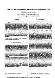
quality of stereoscopic images. 2.1. FTO-RBM Factored Third Order Restricted Boltzmann Machines [14] are stochastic energy-based models, capable of unsupervised learning, which belong to the category of Deep Learning techniques. They were used originally to model the spatial transformation between two successive images [14]. Due to their neural configuration, FTO-RBMs possess excellent generalization and learning capabilities. Different variants of them were used with success in different research areas such for modeling human motion styles [15], for automatically mapping reinforcement learning tasks [16], and pattern recognition [17]. To the best of our knowledge, nobody has managed to employ FTO-RBM to model stereo-pairs, which is the main contribution of this paper. Originally, FTO-RBMs are an extension over Restricted Boltzmann Machines (RBMs) [18] with at least three layers of neurons and factored, multiplicative, three-way interactions between the neurons from different layers. We model a 3D image with a FTO-RBM as depicted in Fig. 1, which consists of: (1) a real valued visible layer l of neurons to code the image perceived by the left eye1 , (2) a real valued visible layer r of neurons to model the image perceived by the right eye, and (3) a stochastic binary hidden layer h. The success of the good encoding, done by FTO-RBM on a stereoscopic image, is guaranteed by the hidden layer which superimpose the other two. This discovers and combines in an unsupervised fashion the important features of the left and right images into its neurons. To learn the inherent relations between these layers three-way undirected connections between all the neurons from different layers are used. To reduce the computational complexity of the model, according to [14], these third order connections are factorized into three matrices of undirected weights. Formally, l = [l1 , . . . , lnl ] and r = [r1 , . . . , rnr ] are real valued vectors, with nl and nr being the numbers of neurons for the left and right visible layer, respectively. h = [h1 , . . . , hnh ] is a binary vector, with nh being the index of the last hidden neuron. Wl , Wr , and Wh are real valued weights matrices of dimensions [nl ×nf ], [nr ×nf ], and [nh × nf ],respectively, where nf is the number of factors. These matrices connect each neuron from the associated layer2 with each factor. Furthermore al , ar , and b represent the biases for the visible left, visible right and the hidden layer, respectively. By convention, in the following equations, X ◦Y is the Hadamard product (the element-wise product) between matrix X and Y , and X T represents the transpose of matrix X. 1 Please not that the image can be mapped directly into the visible neurons, by putting the RGB values for each pixel into a corresponding neuron, or by splitting the image in smaller rectangles and mapping the mean and the standard deviation for each RGB channel for each rectangle into neurons. 2 For a weights matrix the layer is given by the superscript.

Fig. 1: FTO-RBM general architecture, where l, r, and h represent the visible left, visible right, and hidden neurons, respectively. Wl , Wr , and Wh are undirected weights which connect the neurons from the corresponding layer to the factors. al , ar , and b denote the biases for the visible left, visible right and the hidden layer, respectively. # G is used for binary neurons and the other type of units are Gaussian neurons. The total energy function for the FTO-RBM model is written in Equation 1 and it is given by the sum over all possible neurons and their connections: E =lT al + rT ar + hT b X  + (lT Wl ) ◦ (rT Wr ) ◦ (hT Wh )

(1)

f

2.1.1. Inference In FTO-RBMs the probabilistic inference entails the calculation of the three conditional distributions, which correspond to each layer. The first is the probability of the hidden layer conditioned on all the other layers (i.e., p(h|l, r)), the second is the probability of the left visible layer conditioned by the hidden and the right visible layers, while the third one is the probability of the right visible layer given the hidden and the left visible layers, as it is shown in Equation 2. The inference for one layer can be done in parallel for each neuron because there is no direct connection between them.  T
p(h = 1|l, r) = sig b + Wh (lT Wl ) ◦ (rT Wl ) T  p(l|h, r) = N (al + Wl (rT Wr ) ◦ (hT Wh ) , σ 2 ) (2)  T p(r|h, l) = N (ar + Wr (lT Wl ) ◦ (hT Wh ) , σ 2 ) where sig(x) = 1/1 + exp(−x), N represents a Gaussian distribution, and for convenience σ is chosen to be 1 [15]. 2.1.2. Learning & Update Rules The free parameters of the FTO-RBM model Θ (i.e. Wl , Wr , Wh , al , ar , and b) can be fitted, in theory, by using

Maximum Likelihood [19]. Due to the difficulty of computing the derivative of the log-likelihood gradients, Hinton proposed an approximation method called Contrastive Divergence (CD) [20]. In Maximum Likelihood, the learning phase minimizes the Kullback-Leiber (KL) divergence between the input data distribution and the approximating model. In CD, learning follows the gradient of the difference between two divergences [21]: CDn ∝ DKL (p0 (x)||p∞ (x)) − DKL (pn (x)||p∞ (x))

ΥI R

where, pn (.) represents the distribution of a Markov chain running for n steps, and starting from the original distribution p0 (.) of a training data point x. In practice, learning can be performed by running the Markov Chain just for one step, for each data point, in the following manner: (1) infer h by fixing l and r with a training data point x, (2) infer l by using the aforementioned values of h and by fixing r with x, (3) infer r from the previously values of h and by fixing l with x, and (4) update Θ using the update rule from the next equation. Θτ +1 = Θτ + µ∆Θτ + α(∆Θτ +1 − γΘτ )

(3)

where τ , µ, α, and γ represent training epoch, momentum, learning rate, and weights decay, respectively. The interested reader should refer to [22] to gain a further insight on these parameters. Furthermore, the above procedure has to be repeated for an arbitrary number of epochs, until the model converges. The delta rule for each of the free parameters Θ can be computed by deriving the energy function from Equation 1 with respect to each of them, yielding:

  ∆Wh = h (lT Wl ) ◦ (rT Wr ) data

  − h (lT Wl ) ◦ (rT Wr ) recon

  ∆Wl = l (rT Wr ) ◦ (hT Wh ) data (4)

  − l (rT Wr ) ◦ (hT Wh ) recon

  ∆Wr = r (lT Wl ) ◦ (hT Wh ) data

  − r (lT Wl ) ◦ (hT Wh ) recon ∆al = hlidata − hlirecon ∆ar = hridata − hrirecon

• I R is a 3D reference image. • ID = {I1D , ..., InD } is a set of 3D images, derived from I R and exposed to different types of distortions. R • ΥI represents a FTO-RBM learned to model I R . R • lIΥIR is the visible left layer l of ΥI fixed with the left part of any stereoscopic image I. R • rIΥIR is the visible right layer r of ΥI fixed with the right part of any stereoscopic image I. I I represent the inferred neurons values from , r[ • l[

(5)

∆h = hhidata − hhirecon where h.idata and h.irecon represents the configuration of the FTO-RBM at the Markov Chain initialization and after running it for n steps, respectively. 2.2. Q3D-RBM We explain herein our proposed Reduced Reference metric based on FTO-RBM, which we use to automatically assess the quality of 3D images, namely Q3D-RBM. We use the following notations:

ΥI R

R

the visible left and right layers, respectively, of the ΥI model, after a Markov Chain similar with the one deR scribed in Subsection 2.1.2 has been run on ΥI , starting from lIΥIR and rIΥIR . Hence, after a FTO-RBM learns the hidden features of any input data which belong to an original training set (e.g. R ΥI ), it is able to reconstruct those original data with a very small reconstruction error. Besides that, we discovered, based on the properties of RBMs derived models in general, that if other data distributions are fixed into the learned FTO-RBM, the reconstruction error for these distributions will be correlated with the distances between them and the original training set. Thus, the Q3D-RBM metric is given by the reconstruction error of a distorted 3D image pass through a FTORBM learned on a reference 3D image. Furthermore, we have choosen the Root Mean Square Error (RMSE) to measure the reconstruction error, but other statistical measures can be used. Formally, Q3D-RBM is defined in the next equations: r el + er Q3D-RBM(I) = , ∀ I ∈ ID , where nl + nr nl X  [ 2 el = (lI IR )j − (lIΥIR )j (6) Υ j=1 nr X  [ 2 (rI IR )j − (rIΥIR )j er = Υ

j=1

It is worth mentioning, that if we would have a vector Qsubj = [Qsubj (I1D ), ..., Qsubj (InD )] which collect the values of a subjective image quality assessment study, such as DMOS, for all distorted images which belongs to ID , and another vector QQ3D = [QQ3DR BM (I1D ), ..., QQ3DR BM (InD )] which collect the values obtained by Q3D-RBM metric on all images from ID , in the perfect case we can write Qsubj = kQQ3D where k ∈ R. In practice, the aforementioned is not possible, but the experiments presented further show that Q3D-RBM is a good approximation for this relation, having the advantage of a reduced number of parameters need to assess the quality of a 3D image. 3. EXPERIMENTS AND RESULTS To assess the performance of the Q3D-RBM metric we used two benchmark databases with 3D images which have asso-

80

80

70

70

60

60 50 Q3D-RBM

Q3D-RBM

50 40

40

30

30

20

20

10

10

0 0

10

20

30

40 DMOS

50

60

70

80

(a) On IVC 3D Images database

0 0

10

20

30

40 DMOS

50

60

70

80

(b) On Phase II of LIVE 3D database

Fig. 2: DMOS against mapped Q3D-RBM scores. The coordinates for each points represent the quality of a distorted image. ciated subjective studies. For both databases, we have followed a similar procedure and we compared the quality predicted by Q3D-RBM for the distorted stereoscopic images with the values of the objective metrics reported in the original papers, benchmarked in both datasets with the Difference Mean Opinion Scores (DMOS) [23] subjective metric. In both cases, we set for FTO-RBM: nh = 10, nf = 20, α = 10−4 , µ = 0.9, and γ = 0.0002. Furthermore, the training data were normalized to have zero mean and unit variance. Typically, after 300 training epochs the reconstruction error for each of the reference images was smaller than 10−4 . The first experiment was done on the “IVC 3D Images Database” [13]. It contains 6 reference stereoscopic images, each of them being impaired with 15 types of distortions such as JPEG, JPEG2000 compression, and blur filtering at different levels. We split each image from the dataset in small rectangles of 32x32 pixels. The means and standard deviations for each RGB channel of these rectangles were mapped into the visible layers of the FTO-RBM. The computational time to train FTO-RBM was around 6 seconds and to calculate Q3D-RBM for a distorted image was of the order of few milliseconds. As in the original paper [13], the results obtained by the Q3D-RBM metric were normalized to the unitary scale. Furthermore, using indicators of metric performance such as RMSE and Pearson Correlation Coefficient (LCC) between the Q3D-RBM predicted quality and DMOS values associated with the dataset, we assessed the performance of our proposed metric. Fig. 2a depicts the relation between DMOS and the mapped objective scores for Q3D-RBM on each distorted images. In Table 1, the averaged Q3D-RBM scores over all distorted images are presented together with the upper and lower scores for the full reference objectives algorithms from [13]. It can be concluded that Q3D-RBM performs comparably with FF QA metrics, while it is a RR 3D QA metric, independent of distortions type. Table 1: Metrics performance averaged on IVC 3D. Metric RMSE LCC Lower score in [13] (D3) 0.90 0.64 Upper score in [13] (C4) 0.36 0.92 Q3D-RBM 0.29 0.58

The second experiment was done on the Phase II of the LIVE 3D Image Quality Database [12, 24]. This contains 8 reference images with 45 distorted images for each reference one. The distortions are White noise, JPEG2000, JPEG, Gaussian Blur, Fast Fading, each of them having three symmetric distorted stereopairs and six asymmetric distorted stereopairs. To map the images into the FTO-RBM we followed a similar procedure as before and we split the images in rectangle of 40x20 pixels. The time needed to train FTORBM was around 9 seconds per reference image. Additional to the previous experiment we used the Spearman´s rank ordered correlation coefficient. Contrary with the previous experiment, we transformed the Q3D-RBM output to the DMOS scale to be able to assess its performance. Fig. 2b and Table 2 show that Q3D-RBM has a good performance comparable with the full reference metrics. Table 2: Metrics performance averaged on LIVE 3D Phase II Metric RMSE LCC SROCC Lower score in [12] (PSNR 2D baseline) 17.67 0.68 0.67 Upper score in [12] (MS-SSIM Cyclopean) 10.20 0.90 0.90 Q3D-RBM 11.65 0.61 0.66

4. CONCLUSION In this paper we proposed a novel stochastic reduced reference 3D quality assessment metric, namely Q3D-RBM. Notably, it uses Deep Learning concepts to automatically measure the quality of 3D images, for the first time in the IQA literature. Its performance was assess on two subjective benchmarked databases with 3D images. The results showed that our approach yields to a performance comparable with notable full reference quality assessment metrics such as SSIM, MS-SSIM extensions for 3D images. What is most interesting is that we achieve these results through a RR method which has considerable advantages and applicability than FR counterparts. The computational time of few milliseconds and the possibility to assess the quality of a distorted stereoscopic image, without having the original, make Q3D-RBM a suitable solution for on-line multimedia applications. As further directions, we are adapting the mechanism to 3D videos by modeling all the frames of a video with one FTO-RBM.

5. REFERENCES [1] Wei Chen, Jrme Fournier, Marcus Barkowsky, and Patrick Le Callet, “Quality of experience model for 3dtv,” Proc. SPIE, vol. 8288, pp. 82881P–82881P–9, 2012. [2] Stefan Winkler and Praveen Mohandas, “The evolution of video quality measurement: From PSNR to hybrid metrics,” IEEE Transactions on Broadcasting, vol. 54, no. 3, pp. 660–668, Sept. 2008. [3] Vlado Menkovski, Georgios Exarchakos, Antonio Liotta, and Antonio Cuadra Sanchez, “Quality of experience models for multimedia streaming.,” IJMCMC, vol. 2, no. 4, pp. 1–20, 2010. [4] Jing Li, Marcus Barkowsky, Patrick Le Callet, et al., “Recent advances in standardization on 3d quality of experience,” IEEE COMSOCMMTC E-Letter, vol. 8, no. 3, 2013. [5] Anush Krishna Moorthy and Alan Conrad Bovik, “Visual quality assessment algorithms: What does the future hold?,” Multimedia Tools Appl., vol. 51, no. 2, pp. 675–696, Jan. 2011. [6] Vlado Menkovski and Antonio Liotta, “Adaptive psychometric scaling for video quality assessment,” Image Commun., vol. 27, no. 8, pp. 788–799, Sept. 2012. [7] Vlado Menkovski, Georgios Exarchakos, and Antonio Liotta, “The value of relative quality in video delivery,” J. Mob. Multimed., vol. 7, no. 3, pp. 151–162, Sept. 2011. [8] Yoshua Bengio, “Learning deep architectures for ai,” Found. Trends Mach. Learn., vol. 2, no. 1, pp. 1–127, Jan. 2009. [9] Haitham Bou Ammar, Automated Transfer in Reinforcement Learning, Ph.D. thesis, Maastricht University, 2013, Chapter 7. [10] Nicola Jones, “Computer science: The learning machines,” Nature, vol. 505, no. 7482, pp. 146–148, jan 2014. [11] Jonathan Laserson, “From neural networks to deep learning: zeroing in on the human brain.,” ACM Crossroads, vol. 18, no. 1, pp. 29–34, 2011. [12] Ming-Jun Chen, Che-Chun Su, Do-Kyoung Kwon, Lawrence K. Cormack, and Alan C. Bovik, “Fullreference quality assessment of stereopairs accounting for rivalry.,” Sig. Proc.: Image Comm., vol. 28, no. 9, pp. 1143–1155, 2013.

[13] Alexandre Benoit, Patrick Le Callet, Patrizio Campisi, and Romain Cousseau, “Quality assessment of stereoscopic images,” EURASIP Journal on Image and Video Processing, vol. 2008, no. 1, pp. 659024, 2008. [14] Roland Memisevic and Geoffrey E. Hinton, “Learning to Represent Spatial Transformations with Factored Higher-Order Boltzmann Machines,” Neural Computation, vol. 22, no. 6, pp. 1473–1492, Feb. 2010. [15] Graham W. Taylor, Geoffrey E. Hinton, and Sam T. Roweis, “Two distributed-state models for generating high-dimensional time series,” Journal of Machine Learning Research, vol. 12, pp. 1025–1068, 2011. [16] Haitham Bou Ammar, Decebal Constantin Mocanu, Matthew E. Taylor, Kurt Driessens, Karl Tuyls, and Gerhard Weiss, “Automatically mapped transfer between reinforcement learning tasks via three-way restricted boltzmann machines,” in Machine Learning and Knowledge Discovery in Databases, vol. 8189 of Lecture Notes in Computer Science, pp. 449–464. Springer Berlin Heidelberg, 2013. [17] Hugo Larochelle and Geoffrey E. Hinton, “Learning to combine foveal glimpses with a third-order boltzmann machine,” in NIPS, 2010, pp. 1243–1251. [18] P. Smolensky, “Information processing in dynamical systems: Foundations of harmony theory,” in Parallel Distributed Processing: Volume 1: Foundations, D. E. Rumelhart, J. L. McClelland, et al., Eds., pp. 194–281. MIT Press, Cambridge, 1987. [19] John Aldrich, “R.a. fisher and the making of maximum likelihood 1912-1922,” Statistical Science, vol. 12, no. 3, pp. 162–176, 09 1997. [20] Geoffrey E. Hinton, “Training Products of Experts by Minimizing Contrastive Divergence,” Neural Computation, vol. 14, no. 8, pp. 1771–1800, Aug. 2002. [21] Miguel A. Carreira-Perpinan and Geoffrey E. Hinton, “On contrastive divergence learning,” 2005. [22] Geoffrey Hinton, “A Practical Guide to Training Restricted Boltzmann Machines,” Tech. Rep., 2010. [23] M. Pinson and S. Wolf, “Comparing subjective video quality testing methodologies,” in SPIE Video Communications and Image Processing Conference, 2003, pp. 8–11. [24] Ming-Jun Chen, Lawrence K. Cormack, and Alan C. Bovik, “No-reference quality assessment of natural stereopairs.,” IEEE Transactions on Image Processing, vol. 22, no. 9, pp. 3379–3391, 2013.