Deep Sequential Context Networks for Action Prediction - People - RIT

Deep Sequential Context Networks for Action Prediction Yu Kong1 Zhiqiang Tao1 Yun Fu1,2 1 Department of Electrical and Computer Engineering, 2 College of Computer and Information Science. Northeastern University, Boston, MA 02115, USA {yukong,zqtao,yunfu}@ece.neu.edu

Abstract

0

This paper proposes efficient and powerful deep networks for action prediction from partially observed videos containing temporally incomplete action executions. Different from after-the-fact action recognition, action prediction task requires action labels to be predicted from these partially observed videos. Our approach exploits abundant sequential context information to enrich the feature representations of partial videos. We reconstruct missing information in the features extracted from partial videos by learning from fully observed action videos. The amount of the information is temporally ordered for the purpose of modeling temporal orderings of action segments. Label information is also used to better separate the learned features of different categories. We develop a new learning formulation that enables efficient model training. Extensive experimental results on UCF101, Sports-1M and BIT datasets demonstrate that our approach remarkably outperforms state-of-the-art methods, and is up to 300× faster than these methods. Results also show that actions differ in their prediction characteristics; some actions can be correctly predicted even though only the beginning 10% portion of videos is observed.

Full observations

Stacked layers of features

t …

Raw features

… Information transfer

Learned features Raw features

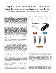
Figure 1. Our DeepSCN predicts the action label given an unfinished action video. Given features extracted from a partially observed video, DeepSCN gains extra discriminative information from fully observed video. Multiple layers of learned features (purple nodes) are stacked to better abstract raw features.

frames of a full video is observed. Action prediction is challenging because decisions must be made based on temporally incomplete action executions. However, certain actions are predictable at their early stage if particular temporal patterns are observed and temporal context is available. Consider, for example, a video of a triple jump. We could imagine that a player is very likely to jump after running since we have seen this type of sport elsewhere1 . The sequential context of the full video observation provides us with the knowledge that the triple jump action consists of running and jumping, and how the action appearance evolves in the temporal domain. This crucial information transferred along temporal axis is the key to action prediction as it helps us to understand the action evolution in the full action observation. In this paper, we propose novel deep sequential context networks (DeepSCN) for action prediction. DeepSCN is based on marginalized stacked autoencoder (MSDA) [4], but extends it to accommodate sequential data. Our deep networks utilize rich sequential context information to better capture the appearance evolution and temporal structure of the full video observations. We learn such information from full videos (see Figure 1), and transfer it to the features extracted from partial videos containing temporally incomplete action executions. This enriches the feature representations, and improves their discriminative power even

1. Introduction Human action recognition has gained significant interests due to its broad applications, such as visual surveillance and video retrieval. This task is to infer the action label after the entire action execution has been observed. However, in some scenarios, predicting the action label before the action execution ends is extremely important. For example, it would be very helpful if an intelligent system on a vehicle can predict a traffic accident before it happens; opposed to recognizing the dangerous accident event thereafter. More importantly, it is essential that the intelligent system can make accurate predictions at the very beginning stage of a video, for instance, when only the beginning 10%

1 We

1

acknowledge that the scene gist also plays an important role here.

though they are extracted from incomplete sequences. The amount of the transferred information at different progress levels2 is temporally ordered for the purpose of modeling the temporal orderings of inhomogeneous action segments. Furthermore, supervisory information is incorporated in DeepSCN in order to improve the discriminative ability of the learned features at different progress levels. DeepSCN has numerous advantages inherited from MSDA: 1) DeepSCN is remarkably faster than existing prediction approaches [13, 2] in training and testing. Empirical results show that DeepSCN is up to 300× faster than [2] and 60× faster than [13]; 2) DeepSCN stacks multiple layers into a deep network that helps effectively summarize action features at different progress levels; 3) it enjoys layer-wise convexity and can be solved efficiently. Our work focuses on short-duration prediction such as “biking” and “diving”, while [17] focuses on long-duration compositional action prediction where an action can be further decomposed into semantic meaningful primitives. For example, an activity “make an omelet” can be decomposed into primitives “crack”, “pour”, “stir”, etc. We simulate sequential data arrival while [2] assumes data are randomly observed in a sequence. We aim at predicting the label for a partially observed video. By comparison, [35, 21, 14] predict what will happen in the future, and [9, 19] localizes the starting and ending frames of an incomplete event.

nique depicts the sequential nature of human activities. Cao et al. [2] generalized human activity recognition. In their work, frames were randomly removed in a video to simulate missing data. They formulated the problem as a posteriormaximization problem, where the likelihood is computed by feature reconstruction error using sparse coding. However, [2] suffers from high computational complexity as the inference is performed on the entire training data. Lan et al. [14] designed a coarse-to-fine hierarchical representation to capture the discriminative human movement at different levels, and used a max-margin framework for final prediction. Kong et al. [13] proposed a structured SVM learning method to simultaneously consider both local and global temporal dynamics of human actions. By enforcing a label consistency of temporal segments, the performance of prediction can be effectively improved. The proposed approach is significantly different from existing action prediction and early detection approaches [24, 13, 2, 14, 9, 19]. The proposed DeepSCN elegantly gains extra sequential context information from full videos to partial videos, while [13, 9, 19] capture increasing confidence score or decreasing detection loss in temporal sequence. Action models are computed by averaging action representations in training data [24], building action dictionaries [2] or describing actions at both coarse and fine levels [14]. By comparison, we build action models by transferring information from full videos in order to improve the discriminative power of partial videos. In addition, our approach stacks multiple feature layers to better summarize action features, while [24, 2, 14, 13] only use hand-crafted features. The prediction of future events was also investigated in other applications, such as predicting events in recommendation systems [16, 23], predicting future visual representation [29], and reasoning about the preferred path for a person [11, 1]. Their goals are different from our work as we focus on predicting the action labels of a video.

2. Related Work Action recognition methods take as input fully observed videos and output labels of human actions. Existing approaches can be roughly categorized into low-level feature-based approaches [15, 33, 30, 22, 31, 20] and midlevel feature-based approaches [12, 26, 34, 36, 18]. Lowlevel features, such as dense trajectory [31] and poselet key-frames [22], utilize local appearance information and spatio-temporal structures, and have shown great success in action recognition. Mid-level feature-based approaches, such as semantic descriptions [12] or data-driven concepts [34], have shown to be capable of recognizing more complex human actions. Furthermore, some deeply learned features [32, 6] were recently proposed to learn high-level information for classification. However, most existing methods expect to observe temporally complete action executions. Their performances are unknown if they are given videos with temporally incomplete action executions. Action prediction methods [24, 2, 14, 13] were proposed to predict the action given a partially observed video. Ryoo [24] proposed integral and dynamic bag-of-words approaches for action prediction. The former one models feature distribution variations over time, while the latter tech-

3. Our Approach Our goal is to predict the action class y of an action video x before the ongoing action execution ends [13, 2, 24]. We follow the problem setup described in [13, 2, 24, 14]. A complete video x containing T frames is uniformly segmented into K segments (K = 10 in this work), mimicking sequential video arrival at various observation ratios. Each T frames. Note that for different videos, segment contains K their lengths T may vary, causing different lengths in their segments. The k-th segment (k ∈ {1, · · · , K}) of the video T + 1]-th frame to the ( kT ranges from the [(k − 1) · K K )-th frame. A temporally partial video or partial observation x(k) is a temporal subsequence that contains the beginning k out of K segments of the video. The progress level g of the partial video x(k) is k: g = k, and its observation ratio

2 The progress level k is the number of observed temporal segments in a video, ranging from 1 to K: k ∈ {1, · · · , K}, where K is the total number of segments in a full video.

2

(k)

(K)

{xi } and their corresponding full observations {xi N X K X

Segment'

1

T

i=1 k=1

A video' x

Partial'video x(k)

(K)

kxi

(k) ¯ (K) − WXk ¯ 2, − Wxi k22 = kX F

} as (1)

where W is a feature transformation matrix of size d × d learned during model training, and k · kF is the Frobenius ¯ (K) is a d × KN matrix containing all the norm. Matrices X ¯ is also a d × KN matrix containing full observations and X all the partial observations:

Progress'level''g = k = 3 Observation'ratio'r = k/K = 0.3

Figure 2. Example of a temporally partial video, and graphical illustration of progress level and observation ratio.

¯ (K) = (x(K) , · · · , x(K) , · · · , x(K) , · · · , x(K) ), X N N {z 1 } |1

k k r is K : r = K (see Figure 2). For a given partial video, its progress level (or level) g and observation ratio r have g = r × K.

¯ = X

{xi , yi }N i=1 ,

Given N training videos we simulate sequential data arrival in this work, and temporally decompose each training video xi into partial observations (k) K {xi }|K k=1 at various progress levels. Note that xi and xi K are the same full video: xi = xi . We would like to learn a feature mapping function G : x(k) → z and a prediction function F : z → y, where x(k) ∈ Rd is a partial video at progress level k, z ∈ RD is the learned feature vector with high discriminative power, and y ∈ Y is the action label.

K times (1) (K) (x1 , · · · , x1 , · · ·

(1) , xN , · · ·

(2)

(K) , xN ).

By minimizing the discrepancy defined in Eq. (1), a par(k) tial observation xi is mapped onto a feature space using the learned projection matrix W under the guidance of its corresponding full observation xK i or xi . The reconstructed (k) feature Wxi is expected to be geometrically closer to its corresponding full observation xK i . Therefore, the learned (k) feature vector Wxi will gain extra crucial information for (K) action prediction from the full observation xi , and its discriminative power is thus enhanced. Note that we use one single feature transformation matrix W here rather than using K transformation matrices, one for each progress level, in order to make our approach compact and practical in testing. If we use K transformation matrices, then we need to know the progress level k of a testing video to pick the right W, which is infeasible in practical scenario. Robust features. During information transfer, noise could be introduced to partial observations, which may degrade the prediction performance. We overcome this problem by regularizing W and constructing robust features for partial videos that are insensitive to noise. Recent work in robust feature learning [4, 28] shows that robust features should be able to be reconstructed from partial and random corruption. Inspired by this idea, we reconstruct features of partial observations with the mapping matrix W:

Visual Features: Our approach works with both deep features and handcrafted features. We extract C3D features [27], or spatiotemporal interest points [5] and dense trajectory features [30] from a partial video x(k) . Bag-of-words model is used to encode handcrafted features.

3.1. Single-layer Feature Learning Sequential context. As shown in [13, 2], it is essential to improve the discriminative power of features extracted from partial observations in order to achieve high prediction performance. This is even more important for predicting the beginning portion of a video since a large amount of useful cues for classification are not observed in the early stage of the video. Furthermore, the features extracted from the beginning portion of a video cannot fully convey the information of the entire video.

N X K X

Intuitively, people are more confident about the action category if more frames are observed. Recent studies [13, 2, 24, 14] show that the best prediction performance is generally made when all the frames are observed. This suggests that full observations contain all the useful information for classification. Motivated by this observation, in this work, we propose to improve the discriminative power of partial videos by gaining extra information from full videos. Our assumption is that if the features from a partial video can be geometrically close to the features from the full video, then their discriminative abilities would be similar. We define the discrepancy between partial observations

i=1 k=1

(k)

kxi

(k)

¯ − WXk ˜ 2, − W˜ xi k22 = kX F

(k)

(3) (k)

˜ i is the corrupted version of the original data xi where x (k) obtained by setting a fraction of the feature vector xi to 0 ˜ is the corrupted version with probability p > 0. Matrix X ¯ defined as of X (1) (K) (1) (K) ˜ = (˜ ˜1 , · · · , x ˜N , · · · , x ˜ N ). X x1 , · · · , x

(4)

To reduce data variance, “infinite” passes of corruptions are performed over the training data [4]. 3

Effectively using “infinitely” many copies of noisy data allows us to learn features robust to noise [4]. In this work, noise may originate from two sources, a partial video itself and the corresponding full video. Although current feature extractors (e.g., C3D and spatiotemporal interest point detectors) have shown to be robust to background noise, the detected features may still be associated with dynamic background that is irrelevant to human actions. In addition, features extracted from human body may also suffer from illumination changes, pose and appearance variations, and camera jittering, etc. This will undoubtedly degrade the representation power of features and further cause significant reduction in prediction performance. By setting random elements in the feature vector xki to 0, these feature elements are removed in the feature vector. This essentially simulates appearance variations in videos, and thus helps in learning robust features. This scheme can be considered as a maskout/drop-out regularization [8, 3]. Label information. Partial observations in the same category may vary greatly in appearance, duration, etc. Therefore, the learned prediction model may not be able to capture complex classification boundaries. We address this problem by incorporating label information to our feature learner, and expect the learned features of partial observations at the same progress level in the same category to be geometrically close to each other. We define the withinclass within-progress-level variance here in order to regularize the learning of parameter matrix W: K N 1X X (k) (k) aij kWxi − Wxj k22 Ψ(W) = 2 i,j=1 k=1

=

K X

(k)

Tr(WX

LX

(k)T

full observation should be decreasing. Such prior knowledge is incorporated using the constraints in optimization problem (7). These constraints also implicitly capture temporal ordering information of inhomogeneous temporal units.

3.2. Model Learning Eq. (7) is a convex problem, and can be solved by the augmented Lagrange method: ¯ − WXk ˜ 2 + αkX ¯ (K) − WXk2 + βΨ (W) L = kX F F +

k=1

(k)

(5)

(8)

3.3. Deep Architecture As suggested by [7, 28, 4], a deep architecture consisting of multiple layers of nonlinearity can improve the representation power of features, especially for classification tasks. Inspired by these studies, we also design a deep structure and nonlinearly map features of partial observations in a layer-wise fashion. This allows us to enhance the effectiveness of matrix W in reconstructing the features at various progress levels. Specifically, using a nonlinear squashing function σ(·) and the learned transformation matrix W at one layer, the new representations of all the partial videos ¯ can be computed by: Z = σ(WX), ¯ where σ(·) is deX fined as tanh(·) in this work. To learn a deep architecture, we stack our single-layer model in Section 3.1 as multi-layer deep networks, and learn the transformation matrices {Wm }M m=1 of M layers using a greedy layer-wise scheme. Specifically, the output of the m-th layer, denoted by Zm , is used as the input for the (m + 1)-th layer (Fig. 3(a)). The transformation matrix Wm+1 of (m + 1)-th layer is then trained after the m-th layer has been trained. For the first layer, the input Z0 is the ¯ Z0 = X. ¯ raw features of all the partial observations X:

(6)

L ∈ R is the label Laplacian matrix: L = D − A. Here, D is the diagonal degree matrix with Dii = PN a , and A is the adjacency matrix that represents the j=1 ij label relationships between training videos. The (i, j)-th element aij in A is 1 if yi = yj and i 6= j; and 0 otherwise. Putting Eq. (1), Eq. (3), and Eq. (5) together, optimal parameter matrix W can be learned by N ×N

¯ − WXk ˜ 2 + αkX ¯ (K) − WXk2 + βΨ (W), min kX F F W

s.t. ∆(k+1) 6 ∆(k) , k = 1, · · · , K − 1,

k=1

Optimization problem in Eq. (9) can be solved by minimizing L with respect to W and maximizing the dual function of L with respect to u iteratively. Thus, W can be ∂L = 0. Please refer to the updated by directly setting ∂W supplementary material for further details.

W ),

(k)

K−1 v X (k+1) (∆ − ∆(k) )2 2

where uk is the Lagrange multiplier corresponding to the kth constraint defined in Eq. (7), and v is a penalty parameter. By introducing ∆ = [∆(2) − ∆(1) , · · · , ∆(K) − ∆(K−1) ]T and u = [u1 , · · · , uK−1 ]T , Eq. (8) is reduced to a compact form: ¯ − WXk ˜ 2 + αkX ¯ (K) − WXk2 L = kX F F v 2 T (9) + βΨ (W) + u ∆ + k∆k2 2 s.t. uk ≥ 0, ∀k = 1, · · · , K − 1.

T

X(k) = (x1 , · · · , xN ) ∈ Rd×N ,

uk (∆(k+1) − ∆(k) ) +

s.t. uk ≥ 0, ∀k = 1, · · · , K − 1,

k=1

where

K−1 X

(7)

where α and β are trade-off parameters balancing the importance of the corresponding terms, and ∆(k) is the reconstruction error ∆(k) = kX(K) − WX(k) k2F . As progress level k increases, the partial video feature x(k) is geometrically approaching the corresponding full video x(K) . Consequently, the amount of information transferred from the 4

3.4. Action Prediction

g

Z = (Z0 , Z1 , · · · , ZM )

Given training videos, DeepSCN is first learned to generate the features of the videos. SVMs with intersection kernel (IKSVM) are then trained to be action predictors using all the feature layers (Z0 , · · · , ZM ) given by DeepSCN. In order to train IKSVM action predictors appropriately, we consider the following two testing scenarios. Scenario 1: Progress level k of a testing video is unknown. This is practical, since in real-world applications, progress levels are always unknown in streaming videos. All the training partial videos are treated to be at the same progress level, and only one IKSVM model is trained. In testing, we use a single IKSVM to predict action labels (Figure 3(b)). Scenario 2: Progress level k of the testing video is known, which was used in [13, 2] but it is impractical in real-world applications. K support vector machines with the intersection kernel are trained for action prediction. The k-th SVM corresponds to partial observations at progress level k. In testing, progress level k of a testing video x is required in order to use the k-th SVM to make predictions (Figure 3(c)). Note that DeepSCN does not require the progress levels of testing videos to be known. Testing. Given a testing video x, DeepSCN is first used to generate the features of the video. Feature z of a testing video is built in a layer-wise fashion (see Figure 3(a)). Specifically, the feature z1 at the first layer is computed by z1 = σ(W1 z0 ) (z0 = x), and then fed into the second layer with parameter W2 . This procedure is repeated until all the features at M layers are computed. Then, the raw feature x and all these learned features are concatenated: z = (z0 , · · · , zM ). Given z, in Scenario 1, the one SVM is adopted to predict the label. If it is in Scenario 2, the k-th SVM from K SVMs will be used for prediction, where k is the progress level of the testing video x.

Z

ZM WM

Action label

(b)

W2

Z1 W1

(a)

g=k Z

(·)

Z0

(c) g = 1

g=k

Action label

g=K

Figure 3. (a) Stacking features for a training/testing video in a layer-wise fashion. Action prediction in two testing scenarios: (b) progress level k is known, and (c) progress level k is unknown.

videos in UCF101 dataset and Sports-1M dataset as C3D model generates features for both segments and full videos. Pre-trained C3D model on Sports-1M dataset is used on UCF101 and Sports-1M datasets. Spatiotemporal interest points (STIPs) [5] and dense trajectory features (DTs) [30] are extracted from partial videos in BIT dataset. Bag-ofwords model (with 500 visual words) is adopted to encode STIPs and DTs features. We follow the split scheme of [27] for UCF101 (split-1) and [10] for Sports-1M datasets, respectively. The first 15 groups of videos in UCF101 are used for training; the next 3 groups for cross-validation; and the remaining 7 groups for testing. We also follow the same experiment settings in [13] for BIT dataset, and use the first 34 videos in each class for training (in total 272 training videos) and use the remaining for testing. Default parameters settings are M = 2, p = 0.5, α = 0.1, β = 0.001 for our method and C = 1 for IKSVMs on all the three datasets if not specified.

4.2. Prediction Performance

4. Experiments

We compare with Dynamic BoW (DBoW) and Integral BoW (IBoW) [24], MSSC and SC [2]3 , and MTSSVM [13]. SVMs with linear kernel, intersection kernel (IKSVM), chi-square kernel, and marginalized stacked autoencoder (MSDA) [4] are used as baselines. IBOW, DBOW, MTSSVM, and all baselines require the groundtruth progress levels to be known in testing. To perform fair comparison, the ground-truth progress levels of testing videos are known to all comparison methods, and all the comparison methods on one dataset are fed with the same features. Scenario 2 in Section 3.4 is adopted and K IKSVMs are trained for our method and MSDA. Note that our method also works without knowing the progress levels. UCF101 dataset. Results in Figure 4(a) show that our method consistently outperforms all the comparison methods, especially at the beginning 5 progress levels. Our

4.1. Dataset and Experiment Setup We evaluate our approach on three datasets: UCF101 dataset [25], Sports-1M dataset [10], and BIT-Interaction dataset [12]. UCF101 dataset consists of 13, 320 videos distributed in 101 action categories. Sports-1M dataset contains 1, 133, 158 videos divided into 487 classes. BIT dataset consists of 8 classes of human interactions, with 50 videos per class. It should be noted that N videos will be 10N videos to action prediction approaches due to the modeling of 10 progress levels. This larger volume of data increases the complexity of the prediction problem. Therefore, we use the first 50 classes in the Sports-1M datasets, and sample 9, 223 videos. This results in 92, 230 partial videos to prediction approaches. Our approach works with both deep features and handcrafted features. We extract C3D features [27] from partial

3 The

5

code is available at http://www.visioncao.com/publications.html.

90

100

70

70

60

50

40

Our method C3D+Linear SVM C3D+IKSVM C3D+Chi-square SVM Integral BoW Dynamic BoW MTSSVM MSSC MSDA

30

20

10

0

0.1

0.2

0.3

0.4

0.5

0.6

0.7

0.8

Observation ratio (a) UCF101 dataset

0.9

1

60

50

40

Our method C3D+Linear SVM C3D+IKSVM C3D+Chi-square SVM Integral BoW Dynamic BoW MTSSVM MSSC MSDA

30

20

10

0

0.1

0.2

0.3

0.4

0.5

0.6

0.7

0.8

0.9

1

Recognition accuracy (%)

90

Recognition accuracy (%)

Recognition accuracy (%)

80

80 70 60 50

Our method C3D+Linear SVM C3D+IKSVM C3D+Chi-square SVM Integral BoW Dynamic BoW MTSSVM MSSC SC MSDA

40 30 20 10 0

Observation ratio (b) Sports1M dataset

0.1

0.2

0.3

0.4

0.5

0.6

0.7

0.8

0.9

1

Observation ratio (c) BIT-Interaction dataset

Figure 4. Prediction results on (a) UCF101, (b) Sports-1M, and (c) BIT dataset. Note that these prediction approaches are optimized for partial videos and thus cannot be directly compared to action recognition approaches given full videos (observation ratio r = 1.0).

comparison methods on 10 observation ratios. Our method remarkably outperforms MSSC and SC [2] in all the 10 cases, demonstrating its ability of learning more discriminative features for action prediction. The most noticeable improvement occurs at r = 0.5 where the performance increases over MSSC and SC are 29.69% and 31.25%, respectively. Our DeepSCN achieves noteably higher performance compared with DBoW and IBoW. We achieve 71.88% accuracy with only the first 40% frames of testing videos being observed, which is higher than DBoW and IBoW at all observation ratios.

method achieves an impressive 45.02% prediction results when only 10% frames are observed, which is 4.97% higher than the MTSSVM. This demonstrates the effectiveness of learning information from full observations in Eq. (1). The performance of our method at observation ratio 0.4 is already higher than the best performance of all the other comparison methods, demonstrating the superiority of our method. It should be noted that DBoW achieves extremely low performance on this dataset. This is possibly because its action models computed by averaging features are not expressive enough to capture highly diverse action dynamics in the same category. Sports-1M dataset. Results in Figure 4(b) demonstrate the superiority of our method over all the comparison methods. Our DeepSCN achieves an impressive 70.23% when only 50% frames are observed, higher than the best performance in 10 cases of all the other comparison methods. Note that DeepSCN makes accurate predictions at an early stage, demonstrating the effectiveness of its deep architecture. DeepSCN outperforms MSDA, showing the benefits of learning extra information from full videos and the monotonic error function. Our method consistently outperforms MTSSVM, MSSC, DBoW and IBoW, suggesting the benefit of learning sequential context information. It should be noted that the performance of our method and C3D+SVM method given full video cannot be directly compared with the original C3D method [27]. We use all the frames in a video in this work while [27] randomly sampled 5 two-second clips from a video. BIT dataset. Results in Figure 4(c) show that our method significantly outperforms all the other comparison methods, especially when 40% or more frames are observed. Our method achieves 71.88% at observation ratio r = 0.4, 5.47% higher than the runner-up MSDA method. At r = 0.6, our method achieves an impressive result of 85.16%, higher than the best performance of all the other

4.3. Running Time Our method is also compared with MTSSVM [13] and MSSC [2] in terms of running time. We executed their authors’ MATLAB code on a 3.4GHz CPU with 64GB RAM, and report the total training and testing time4 in Table 1. Results indicate that our method is significantly faster than the state-of-the-art MTSSVM and MSSC methods. On UCF101 dataset, our method (2 layers) spends 4 hour in training and testing, which is 35× faster than MTSSVM and 105× faster than MSSC. On Sports-1M dataset, our method (2 layers) is 20× faster than MTSSVM, and 308× faster than MSSC. The majority of our time spends in training the SVM action predictors. Training our DeepSCN method only costs 0.05 hours per layer on UCF101 dataset. Our method (3 layers) only takes 7 seconds (0.002 hours) in training and testing on BIT dataset, 60× faster than the MTSSVM and 100× faster than the MSSC method.

4.4. Instantly, Early, and Late Predictable Actions It should be noted that actions differ in their prediction characteristics. Discriminative patterns of actions may ap4 The training times of our method includes the training of DeepSCN and intersection kernel SVMs.

6

661 662 663 664 665

pear early or late in an action video. This affects the portion

to the percentage ofstreaming their testing samples that fallthe in one the (no-SR method), one with ↵ = 0 in (7), levels of testingthe videos areEq. unknown in category real- 745of 738 IP, or= LP. “JavelinThrow” has 29% testing sam746 withEP, scenario. 0, For andInexample, the without theweconstraints in the world thisone experiment, evaluate our method 739 ples all the LPmethod). actions) thatare areunknown late predictable 747 optimization problem (7) other (no-CS The averaged in a (higher practicalthan scenario, i.e. progress levels 740 748 prediction over 10frames observation ratios and prediction (more thanresults 50% video to be in to make in testing. We following the need setting in observed Scenario 1 order defined 741 749in results 2. over the10 beginning 5 observation ratios are summaaccurate prediction). best viewed in color. Table Top early,isvideos and late predictable in Section 3.4. instantly, AllThis the figure partial are treated toactions be 742 750 rized in Table 4. Our method significantly outperforms the UCF101 dataset. Per.level, is the percentage (%) testing samples 743 at the same DeepSCN onlyof one single 751 no-SR methodprogress by 11.31% in the averaged and results, demonthat is instant,isearly or late predictable. SVM trained toofpredict action label from (the ONE 752 744 stratingmodel the effectiveness learningthe robust features method). performance compared withgap twobetween other meth- 753 745 the partial Its observation itself. isThe performance Instantly Predictable Early Predictable Late Predictable ods that require be given in testing: the 754 746 our method and theprogress (↵ = 0) levels methodto shows the importance 755 of learning information from levels full observations. By setting RAND method (progress are randomly generated) 747 Billiards Fencing JavelinThrow and the TRUE method (ground truth progress levels are 748 IceDancing FrisbeeCatch HighJump in the testing phase). Both of the RAND and FrontCrawl TRUE 749 7 used RockClimbingIndoor SoccerPenalty methods train DeepSCN and K SVMs described in ScePlayingPiano VolleyballSpiking HeadMassage 750 nario 2 in Section 3.4. 751 PommelHorse HulaHoop Haircut 752 Performance variations of the three methods on UCF101, Rowing FieldHockeyPenalty 753 Sports-1M, and BIT datasets are shown in Table PlayingViolin 3. ReSkijet HandstandWalking 754 sults show that the averageBasketballDunk performance variation between JugglingBalls CliffDiving PoleVault 755 the TRUE method and the ONE method is within 1% on

can be considered as the most challenging class for predic691 684 4.5.needs Unknown Known Progress Levelclassified of a video that to testing bevsobserved being 692 tion as 29% of its samplesbefore require more than 50% 685 693 Previous assume that the progress levels correctly, i.e., the predictability an action. video frames to beexperiments observedof in order to make accurate pre-of 686 694 testing videos known toof our method,35.45% which may not Inthe all the are 3783 testing samples, testing analyze predictability actions in UCF101 687 Wediction. 695 be are practical. In this experiment, evaluate our method samples instantly and we 62.46% early pre688 dataset, and study at whatpredictable, stage an action can beare predicted.

696 in Scenario 1, where progress levels are unknown in testdictable; onlycategories 2.09% are of lateaction predictable. This suggests that 689 We define three to 697 ing. All the partial videos are videos treated toaccording be at the same a majority of action videos predictable canand be only correctly classified 690 progress level, DeepSCN one(IP), single SVM using model their 698 predictability: instantly early preour approach after observing of label the videos; notmethod). neces699 are trained topredictable predict the half action ONE dictable (EP), and late An (the action video is 1.691 Training and testing time (hours) of(LP). comparison methods sary toItsobserve the entire videos.with Ontwo Sports-1M dataset, 700 692 performance is compared other methods that

666 667 Table 668 IP means that the can be predicted after only observon UCF101, Sports-1M, andvideo BIT datasets. number of layers in 669 “equestrianism” is the easiest action and gymnas701 require progress levels to The be given in “artistic testing: the RAND 693 ing thetics” beginning 10%challenging portion ofaction EP means 670method our to 2ison dataset, 2the onvideo. Sports-1M dataset, theUCF101 most for prediction. Onthat BIT 694 is set an action video is not but can be easiest predicted begin6713 on695 dataset, “bow” andIP“pat” are the and if thethe most chaland BIT dataset, respectively.

ning 50% portion of the video is observed. means that an lenging actions, respectively. Please toLPthe supplemental 672 696 Methods UCF101 Sports-1M BIT detailed onand Sports-1M andbe BIT datasets. action material video isfor neither IPresults nor EP, can only predicted 673 697 50h is observed. 0.12h 698 if more[13] than 50% 140h portion of the video 674MTSSVM 4.5. Unknown vs Known Progress Level 699 Top [2]10 IP, EP,420h 770h 675 MSSC and LP actions in UCF1010.2h dataset are 700 Existing5.methods [13, 24, 2]actions assume“Billiards” that the progress 676 listed Results that and Ours in Figure 4h inshow 2.5h 0.002h 701 levels of videos are known in testing (Scenario 2 in Sec677 “IceDancing” are the easiest actions among 101 actions; all

1

0.9

0.8

0.7

715 716 717 718 719 720 721 100 722 90723 80724 70725

0.6

60726

0.5

50

0.4

727 728 40 729

0.3

30

0.2

20

730 731 SoccerJuggling Bowling CricketBowling 10732 TaiChi TennisSwing ThrowDiscus 7 733 734 Figure 5. Top 10 instantly, early, and late predictable actions in 735 UCF101 dataset. Action names are colored and sorted according

678 early ofor their can be This instantly predicted. In our pear latetesting in an samples action video. affects the portion experiment, there areobserved 33 action categories having over 50% of679 a video that needs to be before being classified 680 ofi.e., theirthe respective testing videos instantly predictable (corcorrectly, predictability of an action. 681 rectly classified after only observing 10% of the frames). 4.5. Unknown vs Known Progress Level We analyze the predictability of actions in UCF101 682 736 Figure 5 also shows that all the testing samples in the 10 EP to the percentage of their testing samples falling in the category of dataset, and study at what stage an action can be predicted. Existing methods in [13, 24, 2] assume that the progress 683 737 actions can be early predicted. In fact, there are 87 actions IP, EP, or LP. This figure is best viewed in color. We of over action to levels of videos are known in testing (Scenario 2 in Sec684 define 738 outthree of 101categories actions having 50%videos of theiraccording respective testtion 3.4), 3.4). which This isis an impractical In assumption since thewe eval685 predictability: 739 ing videos thatinstantly are early predictable predictable (less thanearly 50% prevideo tion impractical. this experiment, their (IP), progress of testing videos arescenario unknown(Scenario in real-world 686 framesand needlate to be observed). (LP). The action “JavelinThrow” uate ourlevels method in a practical 1 defined740 dictable (EP), predictable An action video is scenario. this experiment, we levels evaluateare ourunknown method inina testing. 741 bethe considered as the challenging predicin SectionIn3.4), i.e. progress IP687meanscan that video can bemost predicted after class onlyfor observpractical scenario (Scenario 1 defined in Section 3.4), i.e. 688 tion as 29% of its testing samples require more than 50% All the partial videos are treated to be at the same progress742 ing the beginning 10% portion of the video. EP means that progress levels are unknown in testing. All the partial 689 743 video frames to be observed in order to make accurate prelevel. single SVMlevel, model are trained744 an690actiondiction. video isInnot can be predicted if the beginvideos DeepSCN are treated toand be only at the asame progress Deepall IP the but 3783 testing samples, 35.45% testing (the method). ItsSVM performance is compared with two745 ning portionareofinstantly the video is observed. LP means that prean SCN ONE and only one single model are trained to predict 691 50%samples predictable, and 43.78% are early other levels to be given in746 action video is neither IP norareEP, and can only be action methods labels (the that ONErequire method).progress Its performance is com692 dictable; only 2.09% late predictable. Thepredicted remaining pared withthe twoRAND other methods that(progress require progress to 747 18.69% testing samples cannot be is correctly predicted. This testing: method levelslevels are randomly if693 more than 50% portion of the video observed. be given in testing: theTRUE RAND method 694 suggests thatand a majority of action videos candataset be correctly generated) and the method(progress (groundlevels truthareprogress748 Top 10 IP, EP, LP actions in UCF101 are randomly generated) and the TRUE method (ground truth 695 classified5.using our approach after observing the beginning levels are used in the testing phase). Both of the two meth-749 listed in Figure Results show that actions “Billiards” and progress levels are used in the testing phase). Both of the 696 750 50% frames of the videos. On Sports-1M dataset, “equesods train DeepSCN and K SVMs “IceDancing” are the easiest to predict; all of their testing RAND and TRUE methods train DeepSCN and K SVMs 697 751 trianism” is the easiest action and “artistic gymnastics” is Performance variations ofthree the three methods on UCF101,752 samples aremost instantly predictable. our experiment, there 698 the challenging action forInprediction. On BIT dataset, Performance variations of the methods on UCF101, Sports-1M, andBIT BIT datasets are shown in 2. Table are having over and 50%theofmost theirchallenging respec69933 action 753 “bow”categories and “pat” are the easiest Sports-1M, and datasets are shown in Table Re- 2. Re700 testing 754 sults showthat thatthethe average performance variation actions, respectively. refer to(correctly the supplemental masults show average performance variation betweenbetween tive videos instantly Please predictable classified 701 only 755 terial for the results on Sports-1M andframes). BIT datasets. the TRUE andand the the ONEONE method is within 1% on 1% on the TRUEmethod method method is within after observing the beginning 10% Figure 5 UCF101 and Sports-1M datasets, and it is within 3.12% on also shows that 4 actions have all their testing samples early predictable. In fact, there are 38 actions out of 101 actions 7 BIT dataset. This demonstrates that ONE method can be used in practical scenarios without significant performance having over 50% of their respective testing videos that are decrease where the progress levels are unknown. Thanks to early predictable (less than 50% video frames need to be the proposed DeepSCN, partial videos at various progress observed). The action “JavelinThrow” can be considered as levels can be accurately represented, thereby making one the most challenging class to predict as 29% of its testing SVM powerful enough for predicting these partial videos samples are late predictable (more than 50% video frames and making the progress levels unnecessary in testing. In need to be observed), higher than all the other actions. In addition, training ONE method is significantly faster than all the 37, 830 testing partial videos, 35.45% of them are intraining TRUE method as ONE method only trains one stantly predictable, and 43.78% are early predictable; only SVM while TRUE method needs to train K SVMs. The av2.09% are late predictable. The remaining 18.69% partial erage performance gap between RAND method and TRUE videos cannot be correctly predicted. This suggests that method is 2.25% and 0.34% on UCF101 and Sports-1M a majority of action videos can be correctly classified usdatasets, respectively, indicating the robustness of our aping our approach after observing the beginning 50% frames proach to progress levels on the two datasets. The gap inof the videos. On Sports-1M dataset, “equestrianism” is creases to 16.02% on BIT dataset as short video clips (most the easiest action to predict and “artistic gymnastics” is the of videos are less than 100 frames) and non-cyclic actions most challenging action to predict. On BIT dataset, “bow” (such as “push” and “handshake”) are present in the dataset. and “pat” are the easiest and the most challenging actions to Using inaccurate progress levels in testing would confuse predict, respectively. Please refer to the supplemental mateaction predictors, and thus decreases the performance. rial for the results on Sports-1M and BIT datasets. 0.1

0

0

0.1

0.2

0.3

0.4

0.5

0.6

0.7

0.8

0.9

1

4.5. Unknown vs Known Progress Level

4.6. Effectiveness of Components and Parameters

Existing methods in [13, 24, 2] assume that the progress levels of videos are known in testing (Scenario 2 in Sec-

We evaluate the effectiveness of model components in our method, and the sensitivity to the number of layers M 7

Table 2. Prediction results (%) on UCF101, Sports-1M and BIT datasets using RAND, TRUE, and ONE methods. Observation ratios r ∈ {0.1, 0.3, 0.5, 0.7, 1.0}. The average performance is computed over all 10 observation ratios. UCF101 Sports-1M BIT #SVMs avg. 0.1 0.3 0.5 0.7 1.0 avg. 0.1 0.3 0.5 0.7 1.0 avg. 0.1 0.3 0.5 0.7 1.0 RAND K 79.06 43.91 81.37 83.51 83.72 85.23 68.28 54.33 66.58 70.50 72.06 70.71 56.95 13.28 32.81 69.63 78.13 73.44 TRUE K 81.31 45.02 82.95 85.75 87.10 87.63 68.62 55.02 67.76 70.23 71.52 72.49 72.97 37.50 59.38 78.13 86.72 90.63 ONE 1 80.55 44.31 82.77 85.46 86.34 86.65 68.62 56.15 67.22 70.50 71.57 71.84 69.85 33.63 50.00 81.25 85.94 85.94

on UCF101 dataset. The sensitivity results of our method to corruption probability p, and parameters α and β are shown in the supplemental material. Components. We compare with several variants of our full method, including the method without self reconstruction in Eq. (3) (no-SR method), the one with α = 0 in Eq. (7), the one with β = 0, and the one without the constraints in the optimization problem (7) (noCS method). The averaged prediction results over 10 observation ratios and prediction results over observation ratios 0.1, 0.3, 0.5, 0.7, 1.0 are summarized in Table 3. Our method significantly outperforms the no-SR method by 5.7% on average, demonstrating the effectiveness of learning robust features from the partial observation itself. The performance gap between our method and the (α = 0) method shows the importance of learning information from full observations. The variant method (β = 0) loses label information and fails to successfully separate the learned features in different categories, thereby achieving lower performance. The strength of the constraints in Eq. (7) can be seen from the performance variance between our method and the no-CS method. The constraints implicitly capture temporal orderings over inhomogeneous units, which are beneficial for predicting complex actions.

of videos than the beginning portions of videos. At beginning portions of videos (observation ratios r = 0.1 and r = 0.3), the network with M = 3 layers of features outperforms the one with M = 1 layers of features by 3.02% and 3.09%, respectively. The performance gap increases to 3.6% and 3.43% at ending portions of videos (r = 0.7 and r = 1.0), respectively. This is possibly because the raw features are more discriminative in the ending portions of videos than the beginning portions. Stacking more layers in DeepSCN benefits more from the discriminative features, and thus achieves better performance in the ending portions. Table 4. Accuracy (%) of our method on partial videos of observation ratios r ∈ {0.1, 0.3, 0.5, 0.7, 1.0} with layers M ∈ {0, 1, 2, 3}. M = 0 means the proposed DeepSCN is not used.

#Layer M =0 M =1 M =2 M =3

avg. 75.61 76.55 76.45 76.50 81.31

0.1 39.49 40.29 40.10 39.92 45.02

0.3 76.98 78.17 78.14 78.14 82.95

0.5 80.65 81.02 81.21 81.15 85.75

0.7 81.24 82.34 82.18 82.32 87.10

0.1 39.55 42.98 45.02 46.00

0.3 77.27 80.97 82.95 84.06

0.5 80.33 83.53 85.75 87.21

0.7 80.73 84.43 87.10 88.08

1.0 81.58 85.28 87.63 88.71

5. Conclusion This work addresses the problem of predicting the action label of a video before the action execution ends. We have proposed an efficient and powerful approach for recognizing unfinished human actions from videos. Our approach learns extra information from fully observed actions to improve the discriminative power of the features from temporally partial observations. We further improve the representation power of the features by temporally ordering the amount of the information, incorporating label information, and stacking multiple layers of features. Our method is evaluated on UCF101, Sports-1M, and BIT-Interaction datasets, and shows significant improvements with up to 300× faster speed over state-of-the-art methods. An interesting finding shows that actions differ in their predicability. This inspires us to further explore the temporal structures of actions for prompt and accurate prediction in future work.

Table 3. Comparison experiments among variants on partial videos of observation ratios r ∈ {0.1, 0.3, 0.5, 0.7, 1.0}. The average performance is computed over all 10 observation ratios.

Methods no-SR α=0 β=0 no-CS Ours

avg. 75.39 78.96 81.31 83.36

1.0 82.02 82.87 82.87 82.87 87.63

Number of layers M . We also study performance variations given various layers of features. Prediction accuracies of our networks with M ∈ {0, 1, 2, 3} layers are shown in Table 4 (M = 0 means the proposed DeepSCN is not used). Results indicate that the average performance over 10 observation ratios generally improves when more layers are stacked. With only one hidden layer features (M = 1), our method outperforms the method using raw features only (M = 0) by 3.57% on average performance. The performance difference increases to 7.07% when M = 3 layers of features are stacked. Stacking multiple layers of features has slightly higher positive effect on the ending portions

Acknowledgement This work is supported in part by the NSF IIS award 1651902, ONR Young Investigator Award N00014-14-10484, and U.S. Army Research Office Young Investigator Award W911NF-14-1-0218. 8

References

[19] S. Ma, L. Sigal, and S. Sclaroff. Learning activity progression in lstms for activity detection and early detection. In CVPR, 2016. [20] B. Ni, P. Moulin, X. Yang, and S. Yan. Motion part regularization: Improving action recognition via trajectory selection. In CVPR, June 2015. [21] M. Pei, Y. Jia, and S.-C. Zhu. Parsing video events with goal inference and intent prediction. In ICCV, 2011. [22] M. Raptis and L. Sigal. Poselet key-framing: A model for human activity recognition. In CVPR, 2013. [23] C. Rudin, B. Letham, A. Salleb-Aouissi, E. Kogan, and D. Madigan. Sequential event prediction with association rules. In COLT, pages 615–634, 2011. [24] M. S. Ryoo. Human activity prediction: Early recognition of ongoing activities from streaming videos. In ICCV, 2011. [25] K. Soomro, A. R. Zamir, and M. Shah. UCF101: A Dataset of 101 Human Action Classes From Videos in The Wild. Technical report, CRCV-TR-12-01, 2012. [26] Y. Tian, R. Sukthankar, and M. Shah. Spatiotemporal deformable part models for action detection. In CVPR, 2013. [27] D. Tran, L. Bourdev, R. Fergus, L. Torresani, and M. Paluri. Learning spatiotemporal features with 3d convolutional networks. In ICCV, 2015. [28] P. Vincent, H. Larochelle, I. Lajoie, Y. Bengio, and P.-A. Manzagol. Stacked denoising autoencoders: Learning useful representations in a deep network with a local denoising criterion. JMLR, 11:3371–3408, 2010. [29] C. Vondrick, H. Pirsiavash, and A. Torralba. Anticipating visual representations from unlabeled video. In CVPR, 2016. [30] H. Wang, A. Kl¨aser, C. Schmid, and C.-L. Liu. Action recognition by dense trajectories. In CVPR, pages 3169–3176, 2011. [31] H. Wang, A. Kl¨aser, C. Schmid, and C.-L. Liu. Dense trajectories and motion boundary descriptors for action recognition. IJCV, 103(1):60–79, 2013. [32] L. Wang, Y. Qiao, and X. Tang. Action recognition with trajectory-pooled deep-convolutional descriptors. In CVPR, pages 4305–4314, 2015. [33] B. Wu, C. Yuan, and W. Hu. Human action recognition based on context-dependent graph kernels. In CVPR, 2014. [34] Y. Yang and M. Shah. Complex events detection using datadriven concepts. In ECCV, 2012. [35] Y. Zhou and T. L. Berg. Temporal perception and prediction in ego-centric video. In ICCV, 2015. [36] Y. Zhou, B. Ni, R. Hong, M. Wang, and Q. Tian. Interaction part mining: A mid-level approach for fine-grained action recognition. In CVPR, June 2015.

[1] A. Alahi, K. Goel, V. Ramanathan, A. Robicquet, L. Fei-Fei, and S. Savarese. Social lstm: Human trajectory prediction in crowded spaces. In CVPR, 2016. [2] Y. Cao, D. Barrett, A. Barbu, S. Narayanaswamy, H. Yu, A. Michaux, Y. Lin, S. Dickinson, J. Siskind, and S. Wang. Recognizing human activities from partially observed videos. In CVPR, 2013. [3] M. Chen, K. Weinberger, F. Sha, and Y. Bengio. Marginalized denoising auto-encoders for nonlinear representations. In ICML, 2014. [4] M. Chen, Z. E. Xu, K. Q. Weinberger, and F. Sha. Marginalized denoising autoencoders for domain adaptation. In ICML, 2012. [5] P. Dollar, V. Rabaud, G. Cottrell, and S. Belongie. Behavior recognition via sparse spatio-temporal features. In VS-PETS, 2005. [6] Y. Du, W. Wang, and L. Wang. Hierarchical recurrent neural network for skeleton based action recognition. In CVPR, June 2015. [7] G. Hinton and R. Salakhutdinov. Reducing the dimensionality of data with neural networks. Science, 313(5786):504 – 507, 2006. [8] G. E. Hinton, N. Srivastava, A. Krizhevsky, I. Sutskever, and R. R. Salakhutdinov. Improving neural networks by preventing co-adaptation of feature detectors. Technical report, arXiv:1207.0580v1, 2012. [9] M. Hoai and F. D. la Torre. Max-margin early event detectors. In CVPR, 2012. [10] A. Karpathy, G. Toderici, S. Shetty, T. Leung, R. Sukthankar, and L. Fei-Fei. Large-scale video classification with convolutional neural networks. In CVPR, 2014. [11] K. M. Kitani, B. D. Ziebart, J. A. Bagnell, and M. Hebert. Activity forecasting. In ECCV, 2012. [12] Y. Kong, Y. Jia, and Y. Fu. Interactive phrases: Semantic descriptions for human interaction recognition. In TPAMI, volume 36, pages 1775–1788, 2014. [13] Y. Kong, D. Kit, and Y. Fu. A discriminative model with multiple temporal scales for action prediction. In ECCV, 2014. [14] T. Lan, T.-C. Chen, and S. Savarese. A hierarchical representation for future action prediction. In ECCV, 2014. [15] I. Laptev. On space-time interest points. IJCV, 64(2):107– 123, 2005. [16] B. Letham, C. Rudin, and D. Madigan. Sequential event prediction. Machine Learning, 93:357–380, 2013. [17] K. Li and Y. Fu. Prediction of human activity by discovering temporal sequence patterns. TPAMI, 36(8):1644 – 1657, 2014. [18] S. Ma, L. Sigal, and S. Sclaroff. Space-time tree ensemble for action recognition. In CVPR, June 2015.

9