splitting based variation reduction techniques for both inter- connect and gate. .... are assumed to be sized equally and to be free from per- turbation. The gate size ... So, let's assume that sg is normally distributed with a pdf of N(µs,Ïs) and the ...
7B-2
Delay Uncertainty Reduction by Interconnect and Gate Splitting Vineet Agarwal
Jin Sun
Alexander Mitev
Janet Wang
e-mail: {vagarwal, sunj, mitev, wml}@ece.arizona.edu Electrical and Computer Engineering Department University of Arizona Tucson, AZ - 85721 Tel: 520-621-2434 Fax: 520-621-8076 ABSTRACT Traditional timing variation reduction techniques are only able to decrease the gate delay variation by incurring a delay overhead. In this work, we propose novel and effective splitting based variation reduction techniques for both interconnect and gate. We developed a new tool called TURGIS: Timing Uncertainty Reduction by Gate-Interconnect Splitting which reduces the timing variations of a circuit and presents little delay overhead at the primary output. It is shown that using splitting on interconnect can reduce the Chemical-Mechanical Polishing (CMP) induced dishing effect and can result in decrease at an average of 5% in mean interconnect delay in addition to its variation. Improvements of up to 30% are achieved on timing variation for gates of various size while reduction of 55% can be observed in interconnect delay variation.
1.
INTRODUCTION
Since the advent of nanometer technology, the critical dimensions in today’s digital circuits are diminishing continuously. The impact of manufacturing process such as the Chemical-Mechanical Polishing (CMP) at the present leads to random variations in circuit parameters. The standard deviation in circuit response can go as high as 15%-40% of their expected design value [1, 2]. As a result the timing profile of a circuit end up with a ‘wide-spread’ appearance, which in turn causes yield deterioration due to timing violations. Various techniques have been proposed in the literature to encounter the detrimental effects of these random perturbations. Among these, Sizing has been one of the most effective techniques. Intuitively, manufacturing uncertainties in a larger transistor or interconnect will be proportionately less as compared to that of smaller ones. Sizing employs the same principle and assigns various gate and interconnect sizes to minimize the delay variations at the primary outputs of the circuits. A survey of past literature reveals that circuit timing variation reduction has been researched for several years. For example, [3] and [4] use Lancelot to do gate sizing of circuits and yield improvements of 15% are achieved on average. Lagrangian Relaxation is used in [5] to achieve similar results and improvements are also reported when compared to worst
Permission to make digital or hard copies of all or part of this work for personal or classroom use is granted without fee provided that copies are not made or distributed for profit or commercial advantage and that copies bear this notice and the full citation on the first page. To copy otherwise, to republish, to post on servers or to redistribute to lists, requires prior specific permission and/or a fee. Copyright 200X ACM X-XXXXX-XX-X/XX/XX ...$5.00.
1-4244-0630-7/07/$20.00 ©2007 IEEE.
690
case design. [6] reduced the timing violations by using geometric programming. The aforementioned techniques were successful in improving the yield by decreasing the timing variation, but the gain came at a cost: they incurred an increase in circuit area (transistor drain-source area) and had an increase in the mean delay value at the outputs. This is because sizing up gate is the direct cause of the increase in the gate capacitance. In [7] the authors provide a trade-off between the mean value of the delay and its variance while doing gate sizing on the worst negative statistical slack path of a circuit. As one of the first papers, [8] proposed a gate splitting mechanism during the placement stage to reduce the timing variation with trade-off between variation reduction and area increase. In this paper, we propose a interconnect-gate splitting technique to reduce the timing variations that come from manufacture process such as CMP. Our major contributions are listed as follows. 1) We include interconnect splitting to reduce the variability caused by CMP. As pointed out by [9], interconnect delay has become comparable to gate delay and its delay variation cannot be neglected. 2) We provide mathematic proofs to reveal the relationship between delay variation reduction and splitting. We demonstrate that due to correlation there exists a beneficial design space which decides whether or not to split any particular gate or interconnect. 3) The proposed methodology has been implememted in our new tool TURGIS: Timing Uncertainty Reduction by Gate-Interconnect Splitting. Integrated with existing statistical static timing analysis (SSTA) tool, TURGIS can provide a list of split candidates to placement algorithms such as the spin-off gate placement algorithm in [8]. And with the gate-Steiner-tree distance provided by placement algorithm, TURGIS takes into consideration the extra interconnect cost caused by gate splitting. In the process of variation reduction TURGIS doesn’t increase the transistor drain-source area. However there is a nominal increase in cell area due to increased number of gates and extra interconnect lines. Our experimental results show that when applied on local interconnects the variation was reduced by 50% while reduction of 55% was noted for global interconnects for 130nm technology. When applied on standard benchmark circuits and NAND chains improvements of nearly up to 30% in timing variation were recorded. This technique can be applied together with existing variation reduction techniques to provide trade-offs among the mean value of the delay, its variance and the area cost. The rest of the paper is organized as follows. Section 2 introduces the idea of splitting and then provides its implementation on a simple inverter circuit while providing necessary mathematical modeling and proofs to support the results. Section 3 presents the TURGIS algorithm for application on digital circuits and talks about how to integrate with
7B-2
Statistical Timing Analysis of a split circuit. Experimental results are presented in Section 4 while Section 5 concludes our work.
2.
SPLITTING TECHNIQUE
The Splitting techniques described in the current paper are not exactly the same as ”hardware redundancy”. In the traditional hardware redundancy concept, one has one component ie. p1 to start with, and then he/she has two components in which case p1 and p2 with p1 = p2 . The total component size doubles. Just like the name, the splitting techniques in this paper emphasize on ”splitting” itself. That is, the original component p1 splits into two equal size components pc1 and pc2 . The size of pc1 together with the size of pc2 equals the size of p1 . It is obvious to see that splitting keeps the same total component size. We provide the definition of splitting as follows: Definition 1. Splitting is defined as the technique of substituting a parent (larger) entity by two children (smaller) entity of half the parent size and connecting them in parallel in place of the parent entity.
2.1
Interconnect Splitting
Interconnect splitting arises directly from the CMP process. While planarizing the metal layers in the CMP step, the central portion of the wire cross section gets scooped more than the edges. The ”scooping” of the cross section results in increase of interconnect resistance. This is called dishing of interconnect layers as the metal lines take the shape of the dish. Chang [10] described the dishing effect in detail and introduced corresponding models. Figure 1 depicts the cross section of a wire with dishing effect.
R dish
R dish
dh
Oxide
w
Oxide
Metal
Figure 1: Metal Dishing model Rdish is called the dishing radius, w is the metal width, h is the metal height and dh the height of metal lost at the center � of the line. dh can be written as dh(w, Rdish ) = 2
2 − w4 Rdish is assumed to be 4×-6× of the Rdish − Rdish metal width (w). In this scenario the interconnect resistance per unit length is given as ρ � (1) rd = w2 2 2 wh + 0.5w Rdish − 4 − Rdish sin−1 2Rw dish
If a wide metal line (width Wtotal ) is replaced by N number of metal lines connected in parallel each of width Wtotal /N then the effect of dishing can be reduced effectively. The basic idea of interconnect splitting is shown in Figure 2. It can be seen in the figure that the dishing effect is less prominent in narrower metal lines. The parasitic capacitance of the original interconnect and the split interconnect is nearly the same. The only difference is in line resistance. Thus, if dorg is the delay of original wire and dsplit is the delay of the split configuration then dorg = rd (w, Rdish )Ctotal and dsplit = rd1 � · · · �rdN Ctotal where rdi = rd (w/Ns , Rdish ). where Ns is the number of wires into which the original wire is split. Chang in [10] suggested Ns = 3 or 4 to achieve best performance for 0.25 µm technology. In the
691
Figure 2: Interconnect splitting to subside dishing effect
Size = 0.5sg Parent Gate Driver
Size = sg
Driver
Receiver
Receiver
Figure 3: Original Gate before Splitting
Child Gates
Figure 4: Splitting
Gate after
experimental part, we show that similar conclusion can be obtained for deep submicrion technologies.
2.2 Gate Splitting Figure 3 shows a simple connection of an inverter (parent gate) of size sg , while its split inverter equivalent is shown connected in place of parent inverter gate in Figure 4. The size of both the children inverter is 0.5sg . These two figures demonstrate the basic principle of gate splitting. Now the two children gates do not present any extra load on driver gate, since the total size of the children is the same as that of the parent. And similarly the two children do not provide any extra driving power to the receiver. So functionally the parent gate and children gates are equivalent. It is important to state that gate splitting should not be viewed as multi-fingered gates. Multi-fingered gates have fixed distance between any adjancent two gates while gate splitting allows designers to adjust the distance according to the tradeoffs between area cost and delay variations. As gate effective length Lef f (or critical dimension) is the main reason that causes delay variaion, gate splitting in the current paper is used only when gate effective length approaches deep submicron region. The intuition behind gate splitting mechanism is that the variance of the sum of two less-than-perfectly correlated random variables (each random variable represents the delay of each splitted gate) is always less than the variance of the sum of two perfectly correlated ones (the delay of unsplitted gate). The following section will provide a mathematical analysis of the splitting technique and reason out the reduction in variation through it.
2.3 Delay Metric with Splitting Technique The Elmore delay model for circuit sketched in Figure 3 can be represented as: r CR sg (2) where dps is delay at the output of the parent gate. RD is equivalent driving resistance of the driver. CD is self loading capacitance of the driver. CR is input capacitance of the receiver. r is driving resistance of a minimum sized inverter. CL is Load Capacitance of a minimum sized inverter. sg is dps = 0.69 RD CD + (RD + Rw /Ns )(CL + Cw )sg +
capacitance. Rw is wire resistance. Similarly the Elmore delay model for the circuit sketched in Figure 4 can be written as: dcs = 0.69[RD CD + (RD + Rw /Ns )(CL + Cw )(s1 + s2 ) r + CR ] (3) (s1 + s2 ) where dcs is the delay at the output of the split child gate, and s1 and s2 are size of children gate. Mean value of both s1 and s2 is equal to 0.5sg . Now just for analysis purpose driver and receiver gates are assumed to be sized equally and to be free from perturbation. The gate size sg is a function of Lef f and W width of transistors. Since W = N Lef f , where N is a integer ≥ 1. We view gate size sg as a function of Lef f . If Lef f is modeled as a random variable, then sg = f (Lef f ) is also a random variable. We assume that sg has any kind of gaussian or non-gaussian probability distribution. In this analysis we will assume that perturbations are normally distributed because of simplicity of expressions. But the forthcoming proofs can be easily extended to non-gaussian cases. So, let’s assume that sg is normally distributed with a pdf of N (µs , σs ) and the children gates having similar pdf of the form N (µ�s , σs� ) with µ�s = 0.5µs and the correlation coefficient between them being ρ. The values of σs and σs� can be written in form of µs according to (6). With these simplification and disregarding the constant terms the two delay values can be re-written in the form:
values of µs and ρ. For example if the inverter gate sizes are assumed to be log-normally distributed then we can derive that σ(dcs ) = 0.5360 − 0.1825µs + 0.0217µ2s − 0.0009µ3s σ(dps ) We can see the ratio of delay deviation of the split circuit and that of original circuit is less than 1 for various values of µs within our design range. Figure 5 plots the relative decrease in the delay variance for varying mean gate size (µs ) and correlation coefficient (ρ). We can notice the reduction in delay variation in the split circuit, which exhibits the inherent advantage of splitting any gate. Also, not all the gates will exhibit a decrease in variation due to splitting and thereby splitting those gates can have a detrimental effect on the delay variance. We can thereby choose only those gates for splitting which render positive decrease in delay variance. The region above the dotted line in Figure 5 is called the beneficial design region. A gate is split only if it has the parameters (µs and ρ) which lie in this region. Now 30
ρ=0
25 20
% Decrease in Variaion
7B-2 size of the inverter. N is number of wire split. C is wire s w
Beneficial Design Region
ρ=0.2
15 10
ρ=0.4
Improvement
5 0
ρ=0.6
−5
ρ=0.8
Deterioration −10
dps
�
1 sg + sg
dcs
�
1 sc + sc
Insuitable Design Region
−15 −20 2
3
4
5
6
7
8
9
10
Parent Gate Size
where sc = s1 + s2 . Therefore we can write sc ∼ N (µsc , σsc ) = σs21 + σs22 + 2ρσs1 σs2 . This can be reduced to where σs2� c � σsc = σs 2(1 + ρ) since σs1 = σs2 = σs� . Now for any random variable x with pdf of the form N (µ, σ) we can write � � 2 4 6 σ σ 1 σ 1 +3 + 15 (4) = 1+ E x µ µ µ µ �� � � 2 4 σ σ 1 σ� � + 69 1+8 (5) σ = x µ2 µ µ The proof for this derivation can be found at the end of this section. Now using these values we can write the following: E x+
1 x
1 σ x+ x
1 = E (x) + E x � � � � 1 x+ = �E x � =
σ 2 (x) + σ 2
2
�
1 x
− E2
x+
1 x
+ 2 − 2E (x) E
1 x
(31 − s) % of s (6) 3 This is an empirical model, based on data provided in [1, 2]. Thus a gate of size 1× will have standard deviation of 10% while a gate of size 10× will have standard deviation of 7%. While the transistors of any particular gate will lie close to each other while fabrication, we can safely assume that deviation in critical dimensions of each transistor will be approximately equal due to correlation factors. For x ∼ N (µ, σ) we can assume that σ ≤ 0.1µ according to the model listed in (6). Now re-writing x as (µ + 3σξ), we can deduce that ξ ∼ N (0, 1/3). Now: 1 x
= 0.7282 − 0.0076µs + 0.0077µ2s − 0.0015µ3s
for ρ = 0 while for ρ = 0.5 we can write σ(dcs ) σ(dps )
lets take a look at how to derive (6). First we introduce a size perturbation model. Due to random perturbations while fabricating a circuit, the actual fabricated value deviates from its expected mean value. In this model, the gate sizes have been modeled as normal random variables. It can be intuitively concluded that larger gates will suffer lesser amount of deviation as compared to smaller gates. But the presence of random fluctuations, forbid the decrease of deviation beyond a particular amount, even if we increase the size to large values. In this work, the amount of deviation in the mean value of a gate size of s is assumed to be σs =
If we make x = sg ∼ N (µs , σs ) we can get the value for E(dps ) and σ(dps ) and similarly values for E(dcs ) and σ(dcs ). Using these values and substituting corresponding values of σs and σs� in terms of µs we can write: σ(dcs ) σ(dps )
Figure 5: Change in delay variance of a simple 2 inverter chain for various values of ρ
Now
= 0.8485 − 0.0098µs + 0.0007µ2s − 0.0001µ3s
The derivation for this ratio is omitted here for sake of brevity. Similar expressions can be obtained for non-gaussian cases and can be shown to be less than 1 for various different
692
3σ ξ µ
1 x
=
1 x
�
=
1 1 = µ + 3σξ µ 1+
≤ 1 since max 1 1+ µ � 1 1− µ
3σ ξ µ
σ µ
3σ ξ µ
≤ 0.1, we can write:
−1
3σ ξ+ µ
3σ µ
2
ξ2 −
3σ µ
3
� ξ3 + . . . ∞
Now since ξi ∼ N (0, 1/3), E (ξin ) = 0 for n = 2k + 1 and E (ξin ) = 1.3 . . . (n − 1)σin for n = 2k, where σi = 1/3. � � 2 4 3σ 1 1 3σ 2 4 σi + (1.3) σi + . . . ∞ E = 1+ x µ µ µ 1 x
E
=
∞ 1 1 + µ µ k=1
3σσi µ
2k
(2k − 1)! 2k−1 (k − 1)!
Thus now if we ignore higher order terms we can simplify as: � � 2 4 6 σ σ 1 σ 1 +3 + 15 = 1+ E x µ µ µ µ Following similar steps we can write: � 2 σ σ 1 1 E2 +7 1+2 = 2 x µ µ µ � � � 2 2 1 σ 1 σ E + 15 � 1+3 x µ2 µ µ
4
+ 36
σ µ
4
+ 105
6
σ µ
�
6
�
Therefore again by ignoring higher order terms we can write: �� � � 2 4 6 σ σ 1 σ 1� � +8 + 69 σ = x µ µ µ µ
3.
TURGIS ALGORITHM
Interconnect splitting may be applied on any interconnect at any metal layer with very little extra cost. Splitting gates on the critical path, however, may not be the most optimal choice as we need extra interconnect lines for each gate splitting. We will follow a simple algorithm Timing Uncertainty Reduction by Gate and Interconnect Splitting (TURGIS) to optimally choose the splitting candidates (gates and/or interconnects) for maximum delay variation reduction. This new algorithm may be integrated with statistical static timing analysis (SSTA) to provide a list of split candidates (either gate or interconnect) for spin-off gate placement algorithm [8]. At the same time, the distance between a spin-off gate Gf and steiner tree Ti : df = d(Gf , Ti ) defined in [8] can offer delay estimation adjustment for TURGIS. For example, the delay after splitting in (3) can be modified as dcs = 0.69[RD CD + (RD + Rw /Ns )(CL + Cw )s1 r (RD + (rw df )/Ns )(CL + (cw df ))sf + CR ] (s1 + sf )
(7)
Algorithm 3.1: TURGIS(circuit) 7B-2 ⎧ A ← STA(circuit) ⎪ ⎪ ⎪ ⎪PO ← Extract primary outputs(circuit) ⎪ ⎪ ⎪ ⎪ PI ← Extract primary inputs(circuit) ⎪ ⎪ ⎪ ⎪ for each λ ∈ PO ⎪ ⎪ ⎧ ⎪ ⎪ ⎪ ⎪slpλ = {∅} ⎪ ⎪ ⎪ ⎪ PUSH(slpλ , λ) ⎪ ⎪ ⎪ ⎪ ⎪ ⎪ ⎪ ⎪parent node ← λ ⎪ ⎪ ⎪ ⎪ ⎪ ⎨while parent node ∈ ⎪ / PI ⎪ ⎧ ⎪ do ⎪ ⎪ fan-ins ← Find Fan-In(parent node) ⎪ ⎨ ⎪ ⎪ ⎪ ⎨ ⎪ ⎪ ν ← FIND LARGEST(fan-ins) ⎪ ⎪ do ⎪ ⎪ ⎪ ⎪ PUSH(slp ⎪ λ , ν) ⎪ ⎪ ⎪ ⎩ ⎪ ⎩ ⎪ ⎪ parent node ← ν ⎪ ⎪ ⎪ ⎪ for each g ∈ slp ⎪ ⎪ ⎧ ⎪ ⎪ sg ← Compute Sensitivity(g) ⎪ ⎪ ⎪ ⎪ ⎪ ⎪ ⎪ ⎨if sg > threshold ⎪ ⎧ ⎪ ⎪ ⎪ do ⎨R ← Locate(g) ⎪ ⎪ ⎪ ⎪ ⎪ ⎪ if R ⊂ BeneficialDesignRegion then ⎪ ⎪ ⎩ ⎪ ⎩ ⎪ ⎪ then circuit ← Split(g) ⎪ ⎩ return (circuit) We require two operations in TURGIS: random variable comparison (in FIND LARGEST()) and sensitivity computation (in Compute Sensitivity( )). After running SSTA to get all the delay PDF at the output of gates, we need to identify the statistical longest path by comparing delays. As delays are random variables, we compare two random variables following Theorem 1[11]. Theorem 1. For any 2 random variables x and y, x is (µx −µy ) termed as statistically larger than y if √ 2 2 ≥ 3 or otherσx +σy
(µy −µx ) wise y is termed as statistically larger than x if √ 2 2 ≥ 3 σx +σy
≥ and if none of the above conditions is true then ∂Υ(x,y) ∂x ∂Υ(x,y) ⇒ x ≥ y where the function Υ(x, y) is defined as ∂y � following α = σx2 + σy2 , β = (µx − µy ) /α, ξ1 = µx φ(β) + µy φ(−β) + a ϕ(β), ξ2 = (µ2x + σx2 )φ(β) + (µ2y + σy2 )φ(−β) + (µx + µy ) α ϕ(β), Υ = ξ2 − ξ12 , ϕ(α) = �α ϕ(t)dt −∞
693
andφ(α) =
. Now lets take a look at sensitivity computation. For any circuit with N elements and with size profile as S = {s1 , s2 , . . . , sN }, the output delay can be modeled in form of do (S) = α +
N i=1
Here rw and cw are the per unit length wire resistance and capacitance respectively. df is the distance between a spinoff gate Gf and steiner tree Ti and sf is the size of spin-off gate. Since our aim is to reduce the overall timing variance of a circuit, we can apply splitting to those elements (gates or interconnects) which contribute most to output delay variance. The algorithmic flow of decision making on the choice of circuit elements is outlined in Algorithm 3.1. As the circuit elements on the critical path contribute most to the delay and finding critical path deterministically can lead to false critical path [7], we trace the critical path statistically from each primary output after SSTA. Once all the elements on statistically longest path are identified, sensitivity is assigned to each of those elements. And at last all the elements above the sensitivity threshold are chosen to be split. Also, gates with detrimental effect of splitting (which are not in beneficial design region) are excluded from this list. Lower the value of this threshold, more number of elements will be selected for splitting.
2
α √1 e− 2 2π
βi si +
N i=1
γi s2i +
N −1 N
δij si sj
(8)
i=1 j=i
The coefficients of the (8) can be found out by any technique such as Response Surface Modeling [12] or least square fitting techniques. We have found that for performing least square fit with high accuracy and with least number of sample points, one can make choice of sample points termed as collocation point, as defined in [13]. After do is constructed as a function of s1 , s2 , . . . , sN the following steps can be followed to compute the sensitivity of each element (gi ) of size si . F (S) µ(do ) σ 2 (do ) µ(do |si ) sen(gi )
= fs1 s2 ··· sN (s1 , s2 , · · · , sN ) � � � = · · · do F(S)ds1 ds2 · · · dsN � � � = · · · [do − µ(do )]2 F(S)ds1 ds2 · · · dsN � � � = · · · do F(S|si )ds1 · · · dsi−1 dsi+1 · · · dsN � 1 = [µ(do |si )]2 f (si )dsi σ 2 (do )
Aj
djo
Ai
Line resitance Std. Deviation (ohm/m)
Mean value of Line Resistance (ohm/m)
Figure 7: New Arrival time model for SSTA
2.5
1
2 3 4 5 6 Number of Splits
7
8
A2 o
9
Figure 8: Mean Interconnect Resistance per unit length
4
6
x 10
5
3
2
0
1
2 3 4 5 6 Number of Splits
7
8
9
Figure 9: Standard Deviation of Interconnect Resistance per unit length
Ao = max(Ai + dio , Aj + djo ) But for performing SSTA on the split circuit as sketched in Figure 7 a simple MAX operation cannot be used. In this new case we define Ao as: A1o = max(Ai + d1io , Aj + d1jo ) A2o = max(Ai + d2io , Aj + d2jo ) Ao = min(A1o , A2o ) where Ao is the arrival time at the output node, A1o and A2o are arrival times at the output node of the two child gates, dio and djo are the delay from nodes i and j to o. Where as an superscript of 1 or 2 denote the corresponding delay for the child gates. The rationale behind using a MIN operation is that the output node starts to switch the moment any one of the child gates starts to switch. Therefore the delay at that output node becomes the minimum delay of the two inverter. This can also be confirmed using SPICE simulations. MAX operator can be implemented as multiplication of Cumulative Distribution Function (CDF) of the two arrival times [14]. ⇒
Co (t) = Ca (t)Cb (t)
Where Co (t) is the CDF of output arrival time and Ca (t) and Cb (t) are CDF of input arrival times. Similarly MIN operator can be implemented as Ao = min(Aa , Ab )
⇒
Co (t) = Ca (t) + Cb (t) − Cab (t, t)
where Cab (t, t) is the joint CDF of a and b.
4.
ρ = correlation co−efficient 2.55 ρ=0 ρ=0.2 ρ=0.4ρ=0.6ρ=0.8 2.5
1
2
3 4 5 6 Number of Splits
7
8
9
Figure 10: Effect of correlation on mean interconnect resistance
7
x 10
ρ = correlation co−efficient
6 5
ρ=0.8
4
ρ=0.6 ρ=0.4
3
ρ=0.2
2
ρ=0
1
0
1
2 3 4 5 6 Number of splits
7
8
9
Figure 11: Effect of correlation on interconnect resistance standard deviation
4
where F (S) is the joint probability distribution of the gate sizes and f (si ) is the probability distribution function of si . To include the effects of multi-driver we add on a MIN operator to the methodology. Traditionally the SSTA was performed on circuit as sketched in Figure 6. In this case
Ao = max(Aa , Ab )
x 10
2.45 0
x 10
0
d2io d2jo
2.55
2.45
Ao
Aj
5
2.6
5
2.6
d1jo
Ao
Figure 6: Original Arrival time model for SSTA
4
A1 o
Std. Deviation in line resistance
dio
d1io
Mean Line Resistance
7B-2 Ai
EXPERIMENTAL RESULTS
The implementations were done in MATLAB and HSPICE while the transistor and interconnect model used were the Berkeley PTM model [15]. The timings are reported for an implementation on a computer running Windows OS with 1.5GHz clock frequency and 512Mb RAM. A simple interconnect of length 1 centimeter was chosen for split. This
694
setting will used only for experimentation purposes to show the advantages of splitting. Similar reductions can also be achieved for local and global interconnects of shorter lengths. In this case the wire width (w) and height (h) were assumed to be normal random variables. Rdish was assumed to be 4× the wire width. Figure 8 and Figure 9 show the mean and standard deviation of the resistance of the interconnect line. It is noticed that with increasing number of splits both the mean and the standard deviation of resistance decreases. Variation reduction of up to 55% is achieved. But it becomes nearly constant for splits more than three. Thus we conclude that 3 is the optimal number of splits, as increasing the number of splits will not give us more reduction and will also result in higher cell layout area. Figure 10 and Figure 11 show the effect of spatial distance between the split lines. Since a smaller spatial distance translate to higher correlation coefficient between the widths and heights of the adjacent wires, we see that with increasing correlation coefficient the amount of reduction reduces. For achieving lower correlation coefficient the wires has to be layed out far which causes extra area overhead. Thus there is a tradeoff in amount of reduction achieved and the cell area. The proposed TURGIS was implemented and results are demonstrated for various ISCAS benchmark circuits and Nand chains. The ISCAS circuits were pre-mapped using commercial logic synthesis tool, and then gate sizes were assigned randomly to the gates. TURGIS was then applied on these mapped and sized circuit. First, the primary splitting technique was applied on a Nand chain of various lengths. The results for chain lengths of 5, 10 and 20 are tabulated in Table 1. Two different setting were used for experimentation. At first random sizes were assigned to the gates and next all gates were sized the same (6× in this example). Average improvements of 25% for random sizing and 22% for equal sizing were achieved. Table 2 lists the various output delay statistics values of various ISCAS benchmark circuits for a given gate sizing profile. It also lists the number of gates (N ) present in the circuit. Table 3 lists the delay value statistics if all the gates in the circuit are split. Improvements up to 30% in the variance is recorded while the average improvement recorded was 5.37% in mean value and 21.73% in variance. For TURGIS average improvements are plotted against sensitivity threshold in Figure 12. NC is the number of gates on the statistically longest path and NS is actual number of sensitive gates split. Increasing the sensitivity threshold causes more sensitive gates to be split and results in larger decrease in variance. This can be noticed in Figure 12 that average improvements turn out to be monotonically increasing function of decreasing sensitivity threshold or increase number of sensitive gates split. If the sensitivity threshold is decreased to very small value then generally all the gates on critical paths are selected to be split since the output variance is most sensitive to critical path perturbations and the results approach similar reduction as compared to splitting
Table 1: Results of Gate splitting on various length NAND Original Chain Split Gate Chain Number of Sizing Statistics Statistics gates Profile µ σ σ/µ µ σ σ/µ 5
87.83 1.404 0.015 87.83 1.024 0.011 5 ℵ 82.03 0.949 0.011 81.96 0.805 0.009 10
198.65 3.395 0.016 198.34 2.514 0.012 10 ℵ 175.54 0.995 0.005 175.42 0.847 0.004 20
398.09 3.322 0.008 397.61 2.719 0.006 20 ℵ 362.93 1.121 0.003 362.44 0.756 0.002
⇒ Random Sizing
Table 2: Original Output Delay statistics for ISCAS Benchmark circuits Original Circuit statistics (ps) name NT µ σ (σ/µ) c17 6 42.97 2.98 0.069 c432 160 588.20 33.22 0.053 c499 202 962.49 133.86 0.140 c880 383 200.36 6.26 0.049 c1355 546 1212.65 95.54 0.079 c1908 880 1444.95 159.95 0.100 c2670 1193 410.43 33.38 0.110 c3540 1669 2308.53 52.19 0.032
Table 3: Output Delay statistics for ISCAS Benchmark circuits split on all the gates Split on All gates Improvements CPU Circuit Statistics (ps) (% Decrease) time N name N µ σ (σ/µ) NT ∆µ ∆σ (σ/µ) (sec) c17 6 42.32 2.31 0.054 1 1.51 22.48 21.73 0.02 c432 160 558.26 24.01 0.041 1 5.09 27.72 22.64 0.22 c499 202 915.06 116.42 0.129 1 4.92 13.02 7.85 0.35 c880 383 193.45 5.06 0.038 1 3.44 19.16 22.44 0.51 c1355 546 1156.67 82.55 0.072 1 4.61 13.59 8.86 0.89 c1908 880 1332.45 111.48 0.075 1 7.78 30.30 25.00 2.52 c2670 1193 385.22 23.85 0.085 1 6.14 28.55 22.73 4.21 c3540 1669 2089.71 42.26 0.028 1 9.47 19.02 12.50 19.95 Average Improvements 0 5.37 21.73 17.97
all gates. 30
% Improvement
25
20
15
c432 c499 c880
10
c1908 c2670 5
c3540
Decreasing Sensitivity Threshold Decreasing Sliced Gates 0 0
20
40
60
N /N S
80
100
C
Figure 12: Average Improvements in Output delay variance on ISCAS benchmarks by TURGIS
695
gate chains Improvement (% Decrease) µ σ σ/µ 0.00 27.06 26.67 0.08 15.17 18.18 0.15 25.95 25.00 0.06 14.87 20.00 0.12 18.15 25.00 0.13 32.56 33.33 ℵ ⇒ All gates size = 6
7B-2
5. CONCLUSION In this work, a simple yet effective technique of gateinterconnect splitting was introduced. Interconnect splitting was shown to reduce the variation of the delay by 55%. Preliminary improvements of splitting were demonstrated on inverter gate and disadvantages of previous techniques were overcome. Average improvements of nearly up to 30% were achieved for ISCAS benchmarks and up to 35% were achieved for arbitrary sized Nand gate chains.
6. REFERENCES [1] S. Nassif, “Delay variability: sources, impacts and trends,” in IEEE International Conference on Solid State Circuits, 2000, pp. 368 – 369. [2] S. R. Nassif, “Within chip variability analysis,” in IEDM Technical Digest, 1998, p. 283. [3] S. Raj, S. Vrudhula, and J. Wang, “A methodology to improve timing yield in the presence of process variations,” in DAC, 2004, pp. 448–453. [4] E. Jacobs and M. Berkelaar, “Gate sizing using a statistical delay model,” in DATE, 2000, pp. 283–291. [5] S. H. Choi, B. C. Paul, and K. Roy, “Novel sizing algorithm for yield improvement under process variation in nanometer technology,” in DAC, 2004. [6] J. Singh, V. Nookala, Z.-Q. Luo, and S. Sapatnekar, “Robust gate sizing by geometric prog.” in DAC, 2005. [7] O. Neiroukh and X. Song, “Improving the process variation tolerance of digital circuits using gate sizing and statistical techniques,” in DATE, 2005. [8] D. Wu, G. Venkataraman, J. Hu, Q. Li, and R. Maphapatra, “Dicer: Distributed and cost-effective redundancy for variation tolerance,” in International Conference on Computer Aided Design, 2005. [9] “National technology roadmap for semiconductors,” 2004. [10] R. Chang, “Integrated cmp metrology and modeling with respect to circuit performance,” in Ph.D Thesis, UC. Berkeley, 2004. [11] C. Clark, “The greatest of a finite set of random variables,” Operations Research, vol. 9, no. 2, 1961. [12] R. B. Brawhear, N. Menezes, C. Oh, L. T. Pillage, and M. R. Mercer, “Predicting circuit performance using circuit-level statisticaltiming analysis,” in European Design and Test Conference,, 1994, pp. 332 – 337. [13] S. Isukapalli and P. Georgopoulos, “Stochastic response surface methods (srsms) for uncertainty propagation : Application to enviromental and biological systems,” in Risk Analysis, 1998, pp. 351–363. [14] A. Devgan and C. Kashyap, “Block - based static timing analysis with uncertainty,” in ICCAD, 2003, p. 607. [15] “Berkeley ptm.” [Online]. Available: http://www-device.eecs.berkeley.edu/∼ptm/