In the context of computer vision, matching can be done using correlation measures. This paper presents ..... Four partial correlation measures: â The Zoghlami ...
Dense matching using correlation: new measures that are robust near occlusions Sylvie Chambon and Alain Crouzil TCI, IRIT, UPS, 118 route de Narbonne 31062 Toulouse Cedex 4, FRANCE chambon,crouzil � @irit.fr Abstract
In the context of computer vision, matching can be done using correlation measures. This paper presents the classification of fifty measures into five families. In addition, eighteen new measures based on robust statistics are presented to deal with the problem of occlusions. An evaluation protocol is proposed and the results show that robust measures (one of the five families), including the new measures, give the best results near occlusions.
1 Introduction One of the goals of stereovision is to find the third dimension from two images taken from two different angles. While searching for the third dimension, two other problems occur: calibration and matching. Matching is an important task in computer vision, the accuracy of the three-dimensional reconstruction depending on the accuracy of the matching. The problems of matching are: intensity distortions, noises, untextured areas, foreshortening and occlusions. A lot of matching algorithms have been proposed and compared [7, 8, 18] to take these problems into account. The present paper only deals with matching using correlation measures. In this context, we consider that a correlation measure evaluates the similarity between two data sets: two pixels and their neighbourhoods. Some of the correlation measures (classical measures, derivative-based measures and ordinal measures) have been studied and compared [1, 2, 7, 12, 21, 22]. However, the choice of one correlation measure is difficult so they must first be classified. Here, we are particularly concerned with the occlusion problems and we want to determine the most efficient measures near occlusions. First, the commonly used correlation measures are presented and classified into five families. The measure properties are also given. Second, eighteen new correlation measures that are robust near occlusions are proposed. In a scene, depth discontinuities induce occlusion problems. Pixels with a different depth from the pixel being studied may be considered as outliers. The tools of robust statistics are insensitive to outliers, so, our measures are based on robust statistics. Third, we set up an evaluation protocol that compares all measures. The results are discussed and conclusions drawn.
2 Taxonomy of the measures The two grey level images are denoted by I l and I r and the following notations are used: � The size of the correlation windows is: � 2n � 1 ����� 2m � 1 � and N � 2n � 1 ��� 2m � 1 � , n, m IN and Imax is the maximal grey level;
� I l and I r are the grey levels of the pixels in the left and right images of coordinates xy i j � i � j � and � x � y � and ∇vx y are the gradient vectors at a pixel � x � y � in the image v l � r; � The transposed vector u is uT , � x� is the integer part of x, rank � x � is the rank of x, card � X � is the number of elements in set X and the concatenation is noted: � ; � The vectors f , v l � r, contain the grey levels of the pixels in the left and right v � n; n , q � m; m ; correlation windows: fv �� ����� Iiv� p j � q ����� � T � p
� If ∑n ∑m v P 1� P p ��� n q ��� m ∑A then the LP norms are defined by: � fv � P � ∑A � Ii � p j � q � � P IN . The Euclidean norm is noted: � fv � � � fv � 2 . The scalar product is defined by: fl � fr ∑A Iil� p j � q Ixr� p y � q . The means are noted: fv 1 � N ∑A Iiv� p j � q . The variances are defined by: var � fv �� � fv � fv � 2 . Element i of vector fv is noted f i ; � The Hamming distance is defined by: D � f � f � ∑N � 1 sgn f i � v f i , with sgn � x � 0 r� Ham l r � l i� 0 if x � 0, 1 if x 0 or � 1 otherwise. The measures were classified into five families: cross-correlation-based measures, classical statistics-based measures, derivative-based measures, ordinal measures and robust measures. In tables 1, 2, 3, 4 and 7, the invariance properties (column P) are given. Measures without property are noted 0. The properties are with the scalars a � b � c and d : � M � f � a � f � b� M � f � f � (noted 1); r r � M � afl � bf � M � f � f � l (noted 2); r l l r � M � af � b � cf � d �� M � f � f � (noted 3). r l l r The abreviations (column A BR .), the measure type (column T): similarity (S) or dissimilarity (D) and the intervals of variation (column I) are also given. These intervals are composed of a lower and an upper bound. In the following description, when no explicit reference is given, the reader should consult [1]. Cross-correlation-based measures Three measures use the scalar product (Table 1). NAME
A BR .
Normalised Cross-Correlation
NCC
Zero mean Normalised Cross-Correlation
ZNCC
Moravec
MOR
D EFINITION
I
T
P
� 0; 1�
S
2
� � 1; 1�
S
3
� � 1; 1�
S
0
� fl � fr � ��� fl ��� fr � NCC � fl � fl fr � fr �
2 � fl � fl � � � fr � fr � ����� fl � fl �
2
�
� fr � fr � 2 �
Table 1: Cross-correlation-based measures. Classical statistics-based measures Eight measures use the distances (can be normalised, centered or locally scaled), the variances [3] and the kurtosis [17] (Table 2). NAME
A BR .
Distances
DP
Normalised Distances
NDP
Zero mean Distances
ZDP
Zero mean Normalised Distances
ZNDP
Locally Scaled Distances
LSDP
Variance of Differences
VD
Variance of Absolute P-powered Differences
VADP
Kurtosis
K4
D EFINITION
I
T
P
� 0; Imax P N �
D
0
� 0; Imax P N �
D
0
DP � f l � f l f r � f r �
� 0; Imax P N �
D
1
NDP � fl � fl fr � fr �
� 0; Imax P N �
D
1
P
� 0; Imax P N �
D
0
� 0; Imax 2 �
D
0
P
� 0; Imax 2P �
D
0
� 3 � fl � fr � 2 $
� 0; Imax 4 �
D
0
� fl � fr �
DP � fl fr � �"!
� fl �
P P P P
� fl �#� fl � fr � fr �
� fr �
P P
P
var � fl � fr � var �%$ fl � fr $ � $ � fl � fr �
4
Table 2: Classical statistics-based measures. Derivative-based measures Eight measures (Table 3) use the following filters to compute the image derivatives:
� The Pratt [13], Shen-Castan [4], Sobel, Kirsh and Laplacian of Gaussian filters; � An extension of the Roberts filter: Rr � Ii j � � Ii � 1 j � Ii � 1 j � � � Ii j � 1 � Ii j �
� � Ii�
1�
1 j� 1 �
Ii �
1 j� 1 �
�
� Ii � 1 j � 1 �
Ii �
1 j� 1 �
The filtered image is binarised using an adaptive threshold such that 15% of the region of interest (section 3) are greater than this threshold;
�
� θi j ∆θ �
�
� ∇Ii j �#� Γ with θi j the graotherwise dient vector orientation at � i � j � and ci j lies between 1 and N 2∆π (N , the number θ of the levels with a constant width ∆θ ). The term Γ is a pre-specified threshold level to ignore the low contrast pixels and L is a large value assigned as a code for them. In our tests, the constants are: ∆θ π8 , Γ 10 and L 255 and the distance used is:
� Orientation Code Matching, OCM [19]: c i j
L
�
�
�
�
�� �
�
min � a � b � � N � � a � b � if � a � b � N N� 2 otherwise. The vectors Rs � fv � , Rk � fv � , Rl � fv � , R p � fv � , Rr � fv � and Rocm � fv � are obtained after using Docm � fl � fr �
�
∑iN� � 01 d � fli � fri � with d � a � b �
the Sobel, Kirsch, Laplacian of Gaussian , Pratt, Roberts filters or the OCM respectively. NAME
A BR .
D EFINITION
Seitz 1
SESP
� Rs � fl � � Rs � fr � �
P
Seitz 2
SEKP
� Rk � fl � � Rk � fr � �
P
Nishihara
NIS
Nack 1
NA1
Nack 2
NA2
Pratt
PRATT
Orientation code matching
OCM
Gradient field correlation
GC
I
T
P
� 0; Imax P N �
P
� 0; Imax P N �
P
D 3 D 0
Rl � fl � � Rl � fr � Rr � fl � � Rr � fr � � NRr � fr �
� 0; N �
S
0
� 0; 1�
S
0
NA1 � fl fr � � � NRr � fl � � Rr � fl � � Rr � fr � � ZNCC � R p � fl � R p � fr � �
� 0; 1�
S
0
� 1 � N � Docm � Rocm � fl � Rocm � fr � �
1 � 2 ∑A � ∇li
�
p j q
� ∇rk
�
pl q�
� ∑A ��� ∇li
�
p j q�
Table 3: Derivative-based measures.
�
� ∇rk
�
pl q�
�
�
� � 1; 1�
S
0
� 0;
�
S
0
� � ∞; 1�
S
1
N 2
Ordinal measures Six measures (Table 4) use ordered grey levels of the pixels of the correlation window. This family contains three subfamilies: � The Kaneko measures [10, 11]: b ������� bi ����� � T and c � ����� ci ����� � T , i 0 ��� N � 2 v v with biv
1 0
if fvi � 1 fvi and ci otherwise
1� ci �
� 1
bil �
if i 0 or i even . otherwise
bir �
The matrix C has the weights ci on its diagonal and 0 elsewhere;
�� �
� The Zabih measures [21]: R � f � card � f i f i f N � 2 � i 0; N � 1 � and v � v v rank v N � 2 � f i � with ξ � x � y �� 1 if y Rτ � fv � x or 0 otherwise. v i ξ � fv � The Bhat measures [2]: π is a permutation with π i rank � f i � , i 0; N � 1 and v v v v l � r. A permutation composition s is defined by si πrk , k � πl� 1 � i , where πl� 1 is the inverse of πl . This inverse is defined by: if πli j then � πl� 1 � j i. The deviation i for si is: d i dm ∑ij � 0 J � s j � i � where J � B � 1 if B is true or 0 otherwise. m
NAME
A BR .
Increment Sign Correlation
ISC
Selective Coefficient Correlation
SCC
Zabih (LP norm)
RANKP
Zabih (Hamming)
CENSUS
Bhat and Nayar 1 Bhat and Nayar 2
κ χ
�
D EFINITION � 1 � � N � 1 � � � b l � br � � 1 � bl � � � 1 � br � � C � fl � fl � � � fr � fr � ��� C � fl � fl � ��� C � fr � fr � � � Rrank � fl � � Rrank � fr � �
P P
�
I
T
P
� 0; 1�
S
3
� 0; 1� � 0; N P
1�
S
3
D
3
DHam � Rτ � fl � Rτ � fr � �
� 0; N �
S
3
1 �#� max dmi � � N � 2
� � 1; 1�
S
3
� � 1; 1�
S
3
1�
� � � � �� �� � �
i 0 N 1 � 2dmN 2 �
� N� 2
Table 4: Ordinal measures.
Robust measures Twenty four measures (Table 7) use the tools from robust statistics. Among these measures, there are: � Four partial correlation measures: – The Zoghlami measures [23]: The matrices Av have, on their diagonals, the weights wiv , applied to f vi and 0 elsewhere. The transformation used is: Rα � fv � Av fv and Rα � fv �� 1 � Nv ∑iN� � 01 Rαi � fv � with Nv ∑iN� � 01 wiv and α F1 � F2 . ZNCC is used to obtain a map of the maximal scores. With a threshold, the binarisation of this map gives an occlusion map and finally, ZNCC is used again, with the weights of the occlusion map (F1 ). The threshold is the mean of the image grey levels. The authors proposed other weights: 1 � 2 � ZNCC � fl � fr � � 1 � (F2 ). – The Lan measures [12]: The matrices Aα , α LMS � MV E , have on their diagonals, the weights wiα applied to fvi and 0 elsewhere. The transformation used is: Rα � fv � Aα fv and Rα � fv �� N1α ∑iN� � 01 Rαi � fv � with Nα ∑iN� � 01 wαi . They use a robust line fitting of N data of two dimensions (X � f li fri � T i � 0 N � 1 ) and �� the least median of squares (LMS, the smallest median of the squared residuals) or the Minimum Volume Ellipsoid (MVE, the ellipsoid with the smallest � volume that contains h N � 2� � 1 points of X ); � The quadrant correlation [9]: R � f � sgn � � f � med � f � ��� med f � med � f � � ; q v v v v � � v � The pseudo-norms [6]: the distances (Table 2) with 0 P 1. First, we suggest to normalise and/or center, like for distances (Table 1), the pseudonorms (Table 7) in order to make them more invariant. Second, we propose eighteen new measures using the following tools from robust statistics (Table 7): � The median absolute deviation, MAD; � The least median of squares, the least trimmed squares [15] and the smooth median absolute deviation [14]. We replace the squared differences by the P-powered absolute differences. The ordered values of x are noted: � x � 1:N � 1 ; � x� � Six R-estimators [15, 20] (Table 5): R ∑N � 1 a � rank � f i � f i � ��� f i � f i � . N � 1:N � 1 r r l l k i� 0 k ak � N � 1 � , ∑iN� � 01 ak � i � 0 and The function ak is monotonous with: ak � 0 � ak � i � Jk � � i � 1 ��� � N � 1 � � with � i � 1 ��� � N � 1 � 0 � 1 and 01 Jk � t � dt 0.
�
�
� �
���������
���������
NAME
F UNCTION
Wilcoxon Bounded normal
J1 � t � � t �
�
�
1
�
Optimal B-robust estimator
� t � � 1 4634 � �
J4 � t � � φ
Van der Waerden
�
1�
F UNCTION
�
J5 � t � �
1
� �
�
J3 � t � � sgn � t � � 1 � 2 � �
Median
�� 1� 147� 4φ634� t ifif 00� 3� 9t � � t0� � 309� 61 if 0 � 61 � t � 1 1 � 4634 �� φ � 1� 14 � � ifif 00� 4� 8t � � t0� � 480 � 52 � � if 0� 52 � t � 1 1 � 14
NAME
1 2
J2 � min � 1 4634 max � φ
Minimax
t�
Table 5: The J -functions: φ is the
�
J6 � t � �
1 1 � 2
�
t 05 t 01�
� 0 � 1 � distribution function.
� Eight M-estimators [15, 16, 22] (Table 6): M � f � f � ∑N � 1 ρ � f i � f i � . r k l r i� 0 k l NAME
F UNCTION
��
L1 � L2
ρ1 � x � �
Fair
ρ2 � x � �
Tukey Geman-McClure
�� 11
ρ3 � x � �
�
ρ4 � x � �
NAME
1 � x2 � 2 � 1 � 2 $ x $ � log � 1 �
� � 1� x � � 2 6
$ x$ �
��
if $ x $ 1 otherwise
� x 2 � 2 � � � 1 � x2 �
F UNCTION
�
Cauchy
ρ5 � x � � log � 1 � x2 �
Welsh
ρ6 � x � � � 1 � e x2 � 2 1 35 �%$ x $ � 0 67 �
Huber Rousseeuw
Table 6: The ρ -functions.
�� �
ρ7 � x � �
ρ8 � x � �
�
x2
�
�� �
if $ x $ 1 35 otherwise
� e x � 1 � � � ex � 1 �
NAME
A BR .
I
T
P
Zoghlami and Faugeras 1
ZNCC2
ZNCC � RF1 � fl � RF1 � fr � �
D EFINITION
� � 1; 1�
S
3
Zoghlami and Faugeras 2
ZNCC3
ZNCC � RF2 � fl � RF2 � fr � �
� � 1; 1�
S
3
Reweigthed Zero mean Sum of Squared Differences
RZSSD
ZD2 � RLMS � fl � RLMS � fr � �
� 0; Imax N �
D
1
Reweigthed Zero mean Normalised Cross-Correlation
RZNCC
ZNCC � RMV E � fl � RMVE � fr � �
� � 1; 1�
S
3
Quadrant correlation
QUAD
ZNCC � Rq � fl � Rq � fr � �
� 0; 1�
S
3
Pseudo-norm
PSEUDOP
D
0
Median Absolute Deviation
MAD
Least Median of Powers
LMPP
Least Trimmed Powers
LTPP
Smooth Median Powered Deviation
SMPDP
R-estimators
Rk
M-estimators
Mk
DP � f l f r � , 0
��
∑hi
P
2
� 0; Imax P N �
1
med $ � fl � fr � � med � fl � fr � $
� 0; Imax �
D
3
med ��$ fl � fr $ P �
� 0; Imax P �
D
3
� 0 Imax P h�
D
3
� 0 Imax P h�
D
3
IR
D
3
� 0; � ∞ �
D
0
��
∑hi 1 0 �%$ fl
��
1 0 ��$ fl
� fr $ P �
��
�
∑iN 01 Jk �
��
rank �
fli fri N 1
�
i:N 1
� fr � med � fl � fr � $ P � � � �
�
fli
i:N 1
fri �
∑iN 01 ρk � fli � fri �
Table 7: Robust measures. Properties of the measures The first three families are not robust near occlusions because they use the tools of classical statistics that are very sensitive to outliers. Only centered and/or normalised measures, SESP and GC support intensity distorsions. As the ordinal measures use ranks, they support intensity distortions. They also tolerate outliers. But, these measures can be ambiguous, for example, with these two vectors: u � 0 1 22 35 46 58 61 121 189 � T and v � 0 2 42 60 81 100 123 124 125 � T . When the two vectors are the same (u and u) and when they are different (u and v), the optimal score is obtained: these measures can find erroneous correspondences. The robust measures support intensity distortions. All the new measures are robust near occlusions because they use robust estimators. The ρ -functions of Mk do not have a large value for a large difference of grey level which induces the robustness of Mk . To be robust, the ρ -functions should be constant for large values and grow slowly (like f � x � x) for small values.
3 Evaluation protocol Five pairs of images with ground truth are used but, for space constraints, only three pairs are presented: � The random-dot stereogram: These synthetic images (256 256) contain two planes with an occlusion on the left of the closest plane; � The “map” images (286 216) and the “sawtooth” images (434 380) [18]: These real images were made up piecewise of planar objects (typically posters or paintings, some with cut-out edges). In the disparity maps, the clearer the pixel is, the closer the point to the image plane and the larger the disparity. The black pixels are occluded pixels. All the pairs of real images can be found at: http://www.middlebury.edu/stereo/data.html . Seventeen criteria were chosen: � Percentage of correct and false matches; � Percentage of accepted matches: if the distance between the calculated and the true correspondent is one pixel then the calculated correspondent is accepted. When the percentage of correct matches is low, if this criterion is large then the measure gives a good estimation of the disparities; �
�
�
� Percentage of false positives and false negatives: the measure finds the pixel is matched whereas it is not matched and vice versa;
� Maximum and mean squared errors (in pixels): maximum or mean Euclidean norms between the calculated matched pixels and the true matched pixels;
� Percentage of correct matched pixels in occluded areas: the morphological dilation of the set of pixels with no corresponding pixels in the other image of the pair is considered. The results in the set of pixels without correspondent and in the set of pixels near the pixels without correspondent are distinguished (Figure 1); � Maximum and mean ambiguity and maximum inaccuracy [5] (Figure 2); � Execution time and disparity maps. “Map” images
Random-dot stereogram
“Sawtooth” images
(a)
(b)
(a)
(b)
(a)
(b)
(c)
(d)
(c)
(d)
(c)
(d)
1
P1
P2 Ambiguity
0 P2
0 75P1 15 15 Coordinates of pixels of region of interest 1
�
�
Correlation scores
Correlation scores
(a) Left (b) Right (c) Disparity map (d) Occluded areas, black: pixels without correspondent, grey: region around the black pixels set dilated by the correlation window. Figure 1: Images, ground truth and occluded areas. 1
P2
P1 P3 Inaccuracy
0
0 75P1 15 15 Coordinates of pixels of region of interest 1
P2
�
P3
�
�
Figure 2: Ambiguity and inaccuracy computations. Our algorithm is minimal to highlight only the measure behavior. The parameters of the algorithm are the size of the correlation window and the region of interest. A square correlation window (the size grows from 3 3 to 25 25) and a region of interest limited to the size 61 1 (30 pixels before and 30 pixels after the pixel of interest) are chosen. For each pixel in the left image, the algorithm is: 1. The region of interest is determined in the right image; 2. For each pixel in the region of interest, the correlation score is evaluated; 3. The pixel giving the largest score is the matched pixel. This algorithm only uses similarity measures so each dissimilarity measure is changed into a similarity measure by taking the opposite. Moreover, a bidirectional constraint is added in order to try to locate the occluded pixels. The correlation is performed twice by reversing the roles of two images. The matches for which the reverse correlation falls on the initial point in the left image are considered as valid. �
�
�
4 Experimental results In tables 8 to 10, the following abreviations are used: correct matches (C OR), false matches (FAL), accepted matches (ACC), false positives (FP OS) , false negatives (FN EG), maximal and mean squared errors (M A S E, M SE), maximal and mean ambiguity (M A A, MA), maximal inaccuracy (M A I), correct in the dilated part of the set of occluded pixels (D IL), in the set of occluded pixels (O CC), in the set of pixels near occluded pixels (NO CC) and execution time (T PS). The results are given for the best window size. For each family, one measure that gives the best results is shown (for the robust measures, two measures). In the tables, the best result is emphasised for each column. Random-dot stereogram The first and second families give good results in non-occluded regions (the best are D1 and ZNCC). The derivative-based measures lead to the worst results, except GC (Table 8). The robust measures (in particular RZSSD, RZNCC, PSEUDOP , LTP2 , MAD, SMPD2 , LMP2 , M3 , M4 , M6 and M8 ) give the best results, the percentage of correct matches is high and the maximum and mean square errors are low (Table 8). For the execution time, among the results shown in the Table 8, MAD and GC are the most expensive. In fact, the measures κ , χ , PSEUDOP , RZSSD and RZNCC are the most expensive. Generally, normalised and/or centered measures have a larger execution time than the others. So, these measures should be used only when there are intensity variations between the two images. The larger the window size is, the lower the ambiguity and inaccuracy (Figure 3). In the first family, the normalised and centered measures (ZNCC and MOR) are less ambiguous and inaccurate than the normalised measure (NCC) because the variation interval of ZNCC and MOR is larger than that of the measure NCC. The derivative-based measures give ambiguous and inaccurate results, except GC. Among the ordinal measures, SCC gives good results (one of the best) whereas the other measures give worse results than the other families. For the robust measures, with small window (smaller than 7 7), the partial measures, MAD, LMPP and LTPP have the worst ambiguity and inaccuracy values whereas the PSEUDOP , Mk give the best results (with SCC). ZNCC D1 GC RANK1 MAD LTP2 �
Figure 3: Disparity maps, random-dot stereogram, 7 NAME
C OR (%)
FAL (%)
FP OS (%)
FN EG (%)
ZNCC
97.6
0.7
0.2
1.4
D1
97.7
0.6
0.4
1.3
GC
96
0.8
0.3
2.9
MASE (pix)
�
7.
M SE (pix)
MAA (pix)
MA (pix)
MAI (pix)
D IL (%)
O CC (%)
NO CC T PS (%) (s)
18
0.06
54
0.11
2
81
86
59
10
0.06
59
0.14
4
81
78
59
9
10
0.07
59
0.15
3
83
84
60
40
8
RANK1
96.6
1
0.3
2.1
10
0.09
59
0.15
3
81
79
60
9
MAD
98.4
0.1
0.3
1.2
10
0
60
0.16
5
85
80
61
80
LTP2
98.4
0.1
0.4
1.1
10
0
39
0.13
8
83
73
61
43
Table 8: Random-dot stereogram results, 7 �
7.
“Map” images The results of the first three families are poor near occluded areas. The ordinal measures lead to good results near occlusions but give the worst disparity maps. The new robust measures provide satisfactory results (Table 9) and are not always more expensive than the others (e.g. M1 3 4 7 ). They have the best results near occlusions (Figure 4, the occluded area in the left of the first plane). The measure LTP P , having very good results and a clear disparity map, gives the worst results for ambiguity and inaccuracy, with small windows, because it can attribute a high score (close to the maximum score) to two non-correspondent pixels. κ SMPD2 R3 ZNCC D1 GC
Figure 4: Disparity maps, “map”, 9 NAME
C OR (%)
ACC (%)
FAL (%)
FP OS (%)
FN EG M A S E M SE (%) (pix) (pix)
ZNCC
33
58
58
0.9
8.4
24
D1
33
58
59
0.7
7.7
24
GC
33
59
60
1
6.8
�
9.
MAA (pix)
MA (pix)
MAI (pix)
D IL (%)
O CC (%)
NO CC T PS (%) (s)
0.68
60
0.63
36
67
86
51
0.67
53
1.6
46
70
89
54
11
24
0.74
60
0.38
5
70
82
62
56 419
11
κ
32
49
50
0.5
19
55
0.53
59
0.63
18
70
92
50
SMPD2
35
56
56
0.4
8
23
0.6
60
6.02
60
77
93
64
131
R3
33
58
58
0.7
7.7
24
0.67
54
1.82
46
70
89
54
120
Table 9: “Map” results, 9 �
9.
“Sawtooth” images Near occlusions, the robust measures are again the most efficient (Figure 5, the occluded area in the left of the “sawtooth”). . ZNCC D1 GC SCC LTP2 M3
Figure 5: Disparity maps, “sawtooth”, 9 NAME
C OR (%)
ACC (%)
FAL (%)
FP OS (%)
FN EG (%)
M A S E M SE (pix) (pix)
ZNCC
53
37
40
1.2
6
38
D1
54
37
40
1
6
28
GC
55
37
39
1.5
4
�
9.
MAA (pix)
MA (pix)
MAI (pix)
D IL (%)
O CC (%)
NO CC T PS (%) (s)
0.5
59
0.56
42
61
69
55
0.5
60
2.27
58
64
76
54
29
26
0.5
59
0.16
11
62
62
61
155
29
SCC
53
37
40
1.2
6
38
0.5
60
0.58
41
61
69
55
235
LTP2
54
35
38
0.6
8
30
0.4
60
6.11
60
73
86
64
225
M3
54
38
39
0.8
6
27
0.5
60
0.82
50
68
81
58
276
Table 10: “Sawtooth” results, 9 �
9.
Summary of the results Among all the measures studied, those of the two first families, GC (derivative-based measure) and SCC (ordinal measure) give good results. In contrast, derivative-based measures are not efficient. Ordinal measures that are efficient in occluded regions are not really efficient in non-occluded areas. Robust measures are the most efficient particularly partial correlations, PSEUDOP , MAD, LMPP , LTPP , SMPDP ,
Rk and Mk . However, some of these measures are not as efficient as classical measures in non-occluded areas: the partial correlations, MAD and LMPP . If the execution time, the ambiguity and the inaccuracy are taken into account, the measures MAD, LMPP , LTPP , SMPDP and Rk are less efficient. Finally, with all the tests that have been done, the Mestimator-based measures lead to the best results, the best disparity maps and a reasonable execution time.
5 Conclusion Firstly, this work classifies correlation measures into five families. The description of the properties of these measures can help in the choice of a correlation measure. Then, eighteen new robust measures are proposed. The results show the most efficient measures: the robust measures and in particular, all the M-estimator-based measures. Among the proposed measures, some points might be improved: some measures (LTP P , Rk , MAD and LMPP ) have a high execution time. In fact, the measure implementation was not optimised so the execution times are not the best that can be obtained. A lot of methods can be used to improve this implementation. Moreover, the eighteen new measures can be integrated in a matching algorithm. In fact, robust measures are very efficient near occlusions but some measures, like GC, are more efficient than robust measures in nonoccluded areas. So, our future work will be to develop a robust matching algorithm that will use both robust and non-robust measures.
References [1] P. Aschwanden and W. Guggenb¨ul. Experimental results from a comparative study on correlation type registration algorithms. In F¨orstner and Ruwiedel, editors, Robust computer vision: Quality of Vision Algorithms. Wichmann, Karlsruhe, Germany, March 1992. [2] D. N. Bhat and S. K. Nayar. Ordinal measures for image correspondence. IEEE Transactions on Pattern Analysis and Machine Intelligence, 20(4):415–423, April 1998. [3] G. S. Cox. Template matching and measures of match in image processing. Technical report, University of Cape Town, South Africa, July 1995. http://www.dip.ee.uct.ac.za/imageproc/pattern/. [4] A. Crouzil, L. Massip-Pailhes, and S. Castan. A new correlation criterion based on gradient fields similarity. In International Conference on Pattern Recognition, volume 1, pages 632–636, Vienna, Austria, August 1996. [5] O. De Joinville, H. Maˆıtre, D. Piquet Pellorce, and M. Roux. How to design DEM assessment maps. In Pattern recognition in Remote Sensing Workshop, Andorra La Vella, Andorra, September 2000. [6] J. Delon and B. Roug´e. Le ph´enom`ene d’adh´erence en st´er´eoscopie d´epend du crit`ere de corr´elation. In GRETSI, Toulouse, France, September 2001. (in French). [7] A. Giachetti. Matching techniques to compute image motion. Image and Vision Computing, 18(3):245–258, February 2000.
[8] L. Gottesfeld Brown. A survey of image registration techniques. ACM Computing Surveys, 24(4):325–376, December 1992. [9] P. J. Huber. Robust statistics, chapter 8, pages 204–205. John Wiley & Sons, NewYork, USA, 1981. [10] S. Kaneko, I. Murase, and S. Igarashi. Robust image registration by increment sign correlation. Pattern Recognition, 35(10):2223–2234, October 2002. [11] S. Kaneko, Y. Satoh, and S. Igarashi. Using selective correlation coefficient for robust image registration. Pattern Recognition, 36(5):1165–1173, May 2003. [12] Z. D. Lan and R. Mohr. Robust matching by partial correlation. In British Machine Vision Conference, pages 651–660, Birmingham, England, September 1995. [13] W. K. Pratt. Digital image processing, chapter 20, pages 666–667. Interscience Publication, 1978.
Wiley-
[14] P. J. Rousseeuw and C. Croux. L1 -Statistical Analysis and Related Methods, pages 77–92. Yadolah Dodge, Amsterdam, Holland, 1999. [15] P. J. Rousseeuw and A. M. Leroy. Robust regression and outlier detection. J. Wiley & Sons, New-York, USA, 1987. [16] P. J. Rousseeuw and S. Verboven. Robust estimation in very small samples. Computational Statistics and Data Analysis, 40(4):741–846, October 2002. [17] M. Rziza, D. Aboutajdine, L. Morin, and A. Tamtaoui. Sch´ema multir´esolution d’estimation d’un champ de disparit´es dense sous contrainte e´ pipolaire pour les images bruit´ees. In GRETSI, Toulouse, France, September 2001. (in French). [18] D. Scharstein and R. Szeliski. A taxomomy and evaluation of dense two-frame stereo correspondence algorithms. International Journal of Computer Vision, 47(1):7–42, April 2002. [19] F. Ullah, S. Kaneko, and S. Igarashi. Orientation code matching for robust object search. IEICE Transactions on Information and Systems, E-84-D(8):999–1006, March 2001. [20] Y. Wang and D. Wiens. Optimal, robust R-estimators and test statistics in the linear model. Statistics and Probability Letters, 14:179–188, June 1992. [21] R. Zabih and J. Woodfill. Non-parametric local transforms for computing visual correspondence. In Proceedings of the European Conference on Computer Vision, pages 151–158, Stockholm, Sweden, 1994. [22] Z. Zhang. Parameter estimation techniques: A tutorial with application to conic fitting. International Journal of Image and Vision Computing, 15(1):59–76, January 1997. [23] I. Zoghlami, O. Faugeras, and R. Deriche. Traitement des occlusions pour la modification d’objet plan dans une s´equence d’image. In Actes du congr`es francophone de Vision par Ordinateur, ORASIS, pages 93–103, Clermont-Ferrand, France, May 1996. (in French).