Deployment and Evaluation of a System for Ground-Based ...

468

JOURNAL OF ATMOSPHERIC AND OCEANIC TECHNOLOGY

VOLUME 14

Deployment and Evaluation of a System for Ground-Based Measurement of Cloud Liquid Water Turbulent Fluxes ANDREW S. KOWALSKI, PETER M. ANTHONI,

AND

RICHARD J. VONG

College of Oceanic and Atmospheric Sciences, Oregon State University, Corvallis, Oregon

ANTHONY C. DELANY

AND

GORDON D. MACLEAN

Atmospheric Technology Division, National Center for Atmospheric Research, Boulder, Colorado (Manuscript received 16 May 1996, in final form 11 October 1996) ABSTRACT Direct interception of windblown cloud water by forests has been dubbed ‘‘occult deposition’’ because it represents a hydrological input that is hidden from rain gauges. Eddy correlation studies of this phenomenon have estimated cloud water fluxes to vegetation yet have lacked estimates of error bounds. This paper presents an evaluation of instrumental and methodological errors for cloud liquid water fluxes to put such eddy correlation measurements in context. Procedures for data acquisition, processing (including correction factors), and calibration testing of the particulate volume monitor (PVM) and forward-scattering spectrometer probe (FSSP) are detailed. Nearly 200 h of in-cloud data are analyzed for intercomparison of these instruments. Three methods of coordinate system rotation are investigated; the flux shows little sensitivity to the method used, and the difference between fluxes at different stations is even less sensitive to this choice. Side-by-side intercomparison of two PVMs and one FSSP leads to error bounds of 0.01–0.035 g m23 on half-hour mean cloud liquid water content (relative to typical values of 0.35 g m23) and 2–3.5 mg m22 s21 on the surface-normal liquid water flux (typical magnitude of 7 mg m22 s21 for these data), depending on which instruments are compared.

1. Introduction Recent years have seen an increase in efforts to make in situ measurements of cloud properties from the ground (e.g., Fuzzi et al. 1992; Fuzzi 1994). Groundbased measurements have an economic advantage over aircraft observations in that enormous datasets can be collected by operating continuously at a site where cloud is climatologically frequent. Additionally, interactions of clouds with vegetated surfaces are of interest from the point of view of hydrological and chemical cycling. Various studies (e.g., Beswick et al. 1991; Miller et al. 1993; Vong and Kowalski 1995) have focused on the so-called occult deposition process by which vegetation intercepts windblown cloud water, but this phenomenon remains incompletely understood. Occult deposition is thought to be very important for high-elevation forests; Lovett and Kinsman (1990) summarized estimates of total deposition of sulfate and nitrate for a number of (mostly Appalachian) sites and concluded that occult processes can dominate over wet and dry mechanisms for deposition of these pollutants.

Corresponding author address: Andrew S. Kowalski, College of Oceanic and Atmospheric Sciences, Oregon State University, Oceanography Admin. Bldg. 104, Corvallis, OR 97331-5503. E-mail: [email protected]

q 1997 American Meteorological Society

Occult deposition is prevalent only in regions of variable surface features, that is, near coastlines and at high elevations. Although homogeneous surfaces are preferable for the application of micrometeorological techniques, eddy correlation remains the most plausible method of determining surface fluxes in forested terrain. A ridge top represents a reasonable choice of location for making measurements of cloud water fluxes in that it can be suitably homogeneous in the axial direction, and the flux measured at the summit should represent the integrated effects of cloud–forest interaction over the upwind fetch (downhill; Schuepp et al. 1990). The heterogeneity of the surface suggests a need for multiple measurements of ‘‘point fluxes’’ with spatial separation to characterize broad regions of cloud–vegetation interaction along the ridge axis. Due to the sloping surface, the coordinate system in which fluxes are calculated must be rotated in order to determine the true surface-normal flux at any location in the atmosphere. Selecting the method of coordinate rotation is not trivial; the upwind topography (slope) is dependent on wind direction, which is never truly stationary. Eddy correlation is best applied to conservative atmospheric variables so that sources and sinks are isolated at the surface. Cloud water presents a particular challenge for this technique in that droplets can grow or shrink by a number of processes and achieve sizes

JUNE 1997

KOWALSKI ET AL.

that might not be detected by particular sensors. Pseudoadiabatic theory (Rogers and Yau 1989) predicts that water will change phase between liquid and vapor forms when a (warm) cloud is advected up or down a sloping surface. Unfortunately, measurements of in-cloud fluxes of total water mixing ratio (a conserved variable) are not possible due to limitations on measuring water vapor in a saturated environment (Dabberdt and Schlatter 1996). Vong and Kowalski (1995) observed upward fluxes of the smallest droplets [diameter less than approximately 8 mm, bearing a negligible fraction of the liquid water content (LWC)] concurrent with downward (depositing) fluxes of larger droplets during steady and continuous cloud. This phenomenon also was observed occasionally at Dunslair Heights in Scotland (Beswick et al. 1991) and supports the hypothesis that processes other than deposition are operative on the droplet population near the depositing surface. The precision of eddy correlation liquid water (LW) flux measurements has yet to be addressed. The third field measurement intensive of the Cloud and Aerosol Chemistry Experiment (CACHE-3), conducted from 27 July to 23 September 1994, was designed (a) to intercompare collocated microphysical instruments for the measurement of LWC and LW flux, and (b) to measure LW fluxes at three locations with vertical and lateral separation. This paper details the eddy correlation system deployed and presents an empirical evaluation of instruments and coordinate rotation techniques to put cloud water flux measurements into context. The dataset described here is large relative to previously published studies on cloud droplet fluxes in the surface layer and has sufficient breadth to characterize instrumental and methodological flux errors. These results represent a benchmark for accuracy in the measurement of LWC and LW fluxes from the ground. The following section contains a description of the research site and the instruments. Section 3 describes the data analysis methods including the various rotation schemes investigated and the approach for instrument intercomparison. Section 4 presents results including intercomparison data, flux sensitivity to coordinate rotation method, and a representative time series of cloud water fluxes at the site. The penultimate section discusses these results and defines error bounds for fluxes and LWCs. Finally, conclusions are drawn about the precision of cloud water flux measurements made with the described experimental setup. 2. Experimental a. Description of site, towers, and mounting The Cheeka Peak atmospheric observation station (CPO), maintained by the University of Washington, sits at 460-m elevation on a ridge about 4 km from the Pacific coast on the Olympic Peninsula of Washington. The 6-m-tall canopy, predominantly Pacific silver fir, is

469

FIG. 1. Schematic of the default CACHE-3 instrument configuration (Table 1) for the walk-up and triangular towers. The horizontal boom on the walk-up tower is presented as though vertical to show the instrument mounts.

frequently engulfed in stratiform marine cloud; aerosol and rainwater chemistry in this region is characteristic of the remote marine atmosphere (Vong et al. 1988). During CACHE-3, NCAR’s Atmospheric Surface Turbulent Exchange Research facility (ASTER; Dabberdt et al. 1993) was deployed along with microphysical and turbulence instrumentation from Oregon State University (OSU) to measure LWC and LW fluxes on two towers (denoted hereafter as ‘‘walk-up’’ and ‘‘triangular’’) along the ridge top. A schematic of the towers and instruments used in this study is presented in Fig. 1. Sonic anemometers usually were collocated with the microphysical instruments to determine 3D winds for flux calculations (exceptions are noted below). A host of instruments provided supporting measurements to assist in interpretation of the measured cloud water fluxes; these will be described elsewhere. The ‘‘default’’ configuration for instrument deployment during CACHE-3 placed a forward-scattering spectrometer probe (FSSP) on the walk-up tower boom and two open-path particulate volume monitors (PVM; see instrument descriptions below) at 10 and 15 m on the triangular tower (Fig. 1). Each of three stations was thus equipped for LW flux measurement, with lateral and vertical separation between stations. The walk-up tower supported a 3-m boom, rotatable in the horizontal plane, at 9 m above ground level (AGL); hereafter this station will be referred to as nominally at 10 m. A cross-member on the end of the boom had mounts for a sonic anemometer, the FSSP, and a PVM. The main axis of the FSSP was oriented at 128 below horizontal, tilted into the typical mean wind for the site that comes up the slope during cloud conditions.

470


The FSSP and PVM each were mounted 60 cm from the centrally positioned anemometer. The FSSP was fitted with a custom-designed, cylindrical inlet, tapered to match the instrument’s aspiration velocity to typical mean winds of 8 m s21 at the site and sample isokinetically. Periodic rotations kept the boom pointing into the mean wind during cloud episodes, usually to within 658 (azimuthal angle); a boom direction indicator tracked the orientation of the boom. The triangular tower, a low-profile aluminum structure with 24-cm center-to-center vertical members, stood 28 m to the north-northwest of the walk-up tower (typical wind directions for cloud at the site during CACHE-3 are west-southwest). This tower supported booms for level mounting of the sonic anemometers and PVMs, one of each at 10 and 15 m AGL, facing toward the south-southwest. b. Instrumentation and data processing The ASTER data acquisition modules (ADAMs), situated at the base of each tower, sampled serial data from the FSSP and sonic anemometers (both at 10 Hz) and raw voltages from the PVMs (at 20 Hz). Raw data ingested from the ADAMs were stored and backed up daily. Five-minute means and covariances of the 3D wind components and LWC from the PVMs and FSSP were also stored. The sonic anemometers utilized in this study are orthogonal, three-axis instruments (ATI models SWS2H-3K and SWS-211-3K). Kaimal et al. (1990) showed that this instrument design (including internal software) has reduced probe-induced flow distortion errors (Wyngaard 1981) and transducer shadowing effects (Wyngaard and Zhang 1985) to negligible levels. The sonic electronics averaged their 100-Hz measurements to 10 Hz and transmitted to the ADAMs on a serial line. The cloud microphysical instruments were two PVM100s (Gerber 1991) and an FSSP-100-ER (Knollenberg 1981; Baumgardner 1983). Heintzenberg (1992) reported that of the four methods of measuring LWC examined by the Po Valley team (Arends et al. 1992), the PVM was the preferred instrument for measuring LW mass (or volume), while the FSSP was most useful for examining size-dependent processes. Of the two PVMs deployed, one was on loan from Gerber Scientific Inc. and was termed the GSI PVM; the other was dubbed the OSU PVM. GSI delivered the loaner with the caveat that its calibration differed from that of the OSU PVM by a factor of over 20%, based on 4 min of wind tunnel comparisons. In this study, the OSU PVM consistently has been treated as the standard for LWC measurements because during CACHE-1 it showed excellent agreement with the FSSP for LWC and LW fluxes, except for small flux deviations that were identified as being due to ‘‘wind ramming’’ of the FSSP at high wind speeds (Vong and Kowalski 1995). Field intercomparison data were used (below) to deter-

VOLUME 14

mine a factor of 1.28 by which the GSI PVM was corrected in order to achieve agreement with the OSU PVM. Software routinely deducted the clear-air offset and applied the linear calibration slope to the output of each instrument. The 20-Hz data were averaged to 10 Hz for computing covariances with the 10-Hz sonic wind outputs via the eddy correlation technique (Businger and Delany 1990). Proper operation of an FSSP requires considerable attention; a variety of problems such as failure to determine the sampled air volume, optical misalignment, poor calibration, inlet losses and droplet coincidence (Baumgardner et al. 1985) can lead to large errors in the reported LWC (cf. Valente et al. 1989). The procedure detailed below for operation of a ground-based FSSP and processing LWC and LW flux data yielded excellent agreement with the OSU PVM. An 80386/387 PC with an installed FSSP interface card (1D probe adaptor module, PMS 1058B) and a PCI A/D board interrogated the FSSP according to a BASIC program. An 8-MHz clock generator and 32-bit counter of the A/D board timed the read intervals. Although the nominal sample interval was 100 ms, for precision a more exact measure of the FSSP accumulation interval was recorded. The probe was optimized by the manufacturer for ground-based operation with a flow rate of 23.85 m s21 by increasing the laser beam area to 0.807 mm2 (both values were determined from laboratory measurements immediately prior to CACHE-3). The FSSP functioned in one of two droplet diameter ranges during CACHE-3; predominantly, range 2 was used to measure droplet spectra (2 mm # diameter # 32 mm for 2-mm intervals), but range 1 was used during one cloud event with unusually large droplets (2 mm # diameter # 47 mm droplets for 3-mm intervals). The sample air volume was corrected for the fraction of rejected droplets (those which passed through the edge of the beam) using the ratio of valid to total strobes (the so-called velocity acceptance ratio defined by Dye and Baumgardner 1984). The 15 values of raw counts were corrected for probe activity to account for the fraction of time (during electronic reset) that no sampling occurred, and for droplet coincidence errors (Baumgardner 1983). Probe ‘‘activity’’ is determined as a percentage of actual count rate to a maximum rate (1000 s21). Corrected counts Nc are then computed from raw counts Nr according to Nc 5

Nr , 1 2 0.007A

(1)

where A is the activity in percent. Activity was also used to interpret data; when the activity becomes too high (see results section below), errors can occur due to coincidence of more than one droplet affecting the sensing volume, and the data are flagged. None of the LWC intercomparison data for the FSSP (presented below) were flagged for high activity.

JUNE 1997

471

KOWALSKI ET AL. TABLE 1. CACHE-3 mounting configurations: intercomparison and ‘‘default’’ sampling periods.

Period

Date (1994)

N (30 min)

A

27–29 Jul

39

B

29–31 Jul

13

C

2–4 Aug

110

D

4–6 Aug

44

—

6–15 Aug

119

E

15–19 Aug

79

F

19–23 Aug

124

23 Aug–17 Sep 17–23 Sep

350 68

— G

Mounting configuration PVMs strapped to walk-up tower handrails, normal orientation (1808 to each other, 908 to mean winds) Same as A but GSI PVM rotated 908 with laser pointing into the mean wind PVMs on triangular tower, OSU at 10.75 m, GSI at 10 m PVMs on triangular tower, OSU at 10 m, GSI at 10.75 m ‘‘Default’’ configuration: OSU PVM at 10 m, GSI PVM at 15 m

Flux measured No

Ideal configuration for LWC comparison

No

Anomalous results, see text

Yes

OSU PVM: 75-cm vertical separation from sonic GSI PVM: 75-cm vertical separation from sonic Used in data screening schemes and flux sensitivity to coordinate rotations Ideal configuration for FSSP/ PVM comparison

Yes Yes

OSU PVM/FSSP on walk-up tower. Same as CACHE-1 configuration (Vong and Kowalski 1995) PVMs at 12.5 m on cross arm of flux tower, with 2-m transverse separation

Yes

Default configuration PVMs on 10-m flux tower boom, series configuration; 0.3-m separation in streamwise direction (1808 to each other, 908 to mean winds)

Yes Yes

c. Field calibration procedures The sonic anemometers were calibrated on site using ‘‘zero-air chambers’’ for each axis to establish the sonic wave transit time (between transducers) at zero wind velocity at the station pressure and temperature. To test the hypothesis that the calibrations of the two PVMs did not change over the course of the experiment, regular calibration checks were performed on each instrument. An optical disk scattered the direct laser beam into the receiver optics. Neither instrument showed any significant drift in response to the optical disk over the course of the experiment, and the response of the OSU PVM (for which the disk was designed) was consistent with the calibration data supplied by the manufacturer. The field calibration test procedure for the FSSP demonstrated that it was operating within the manufacturer’s specifications in that the peak in the number distribution obtained from glass calibration beads (Duke Scientific) corresponded to the diameter of the calibration beads (accounting for the change in index of refraction). Counts were sometimes reported in the three smallest size intervals when large beads (diameter greater than 20 mm) were sampled, but such a response was not in evidence in the ambient data (sampling real cloud droplets) based on the monomodal shape of the droplet size spectra, which typically centered around 10–16 mm. The three smallest FSSP size intervals usually contributed less than 1% to the integrated LWC in cloud at CPO. The observed size dependence of the LW flux, including an upward flux of small droplets (cf. Vong and Kowalski 1995), was not consistent with the expected effects of either correlated or uncorrelated noise on the flux for these small size intervals. These three intervals were

Comments

No

Good LWC comparison configuration; high VMD cases excluded Noteable disagreement in LWC, presumed due to configuration; see text

not important to the accurate determination of LWC or LW flux. d. Intercomparison data and configurations The various CACHE-3 microphysical instrument configurations are summarized in Table 1. Some of the intercomparison configurations were not useful for flux determination (the sonic anemometers remained in their fixed locations, described above), and others had no measure of droplet size spectra (FSSP not operating prior to 3 August). For this reason, different types of analyses incorporate data from different intercomparison periods. 3. Methodology a. Statistical comparisons Statistical averaging periods for flux determination have been set at 30 min (Beswick et al. 1991; Vong and Kowalski 1995). This period is sufficiently long to sample a large number of the flux-carrying eddies (found via cospectral analysis to have characteristic timescales of about 20 s at the 10-m sampling height) but short enough to minimize the effects of nonstationarity or trends imposed by synoptic and mesoscale deviations in the flow. Intercomparison analyses were designed to establish error bounds for 30-min LWC and LW flux values. Consistent with the analysis of Vong and Kowalski (1995), the relative standard deviation of LWC (sL/L: L will be used to denote the LWC variable in equations), measured at 10 m AGL by the OSU PVM, was utilized as a screening variable for ‘‘steady cloud.’’

472


Isolating steady cloud simplifies interpretation of fluxes by minimizing the effects of cloud edge or entrainment, screening out periods strongly affected by synoptic variability and focusing on periods where deposition is most likely to represent the dominant process governing the flux. For the sake of the analyses presented below, the steady cloud criterion was used to identify the most stationary periods for performing flux intercomparisons. Two measures to bound errors in half-hour LWC and LW flux are presented. The standard deviation of the difference (between two instruments or two rotation techniques) is used for categorizing random errors, and the mean difference is used to describe bias. These statistics are the two components of the rms difference. For a measurement x, taken by two instruments or techniques, the statistics are related as follows: D [ x 1 2 x 2;

rms [ (D 2)1/2

D 5 D 1 D9;

D 2 5 D2 1 D9 2.

(2)

In these equations, overbars denote Reynolds averages over the ensemble of realizations and primes denote deviations therefrom for individual half-hour values. Here (D92)1/2 is the standard deviation of the difference and D is the mean difference.

a consistent zenith angle based on ensembled realizations of the local-mean method for many cloud events, allowing for variations with wind direction (method 3). The sensitivities of the computed LW flux and betweenstation flux difference to the method of rotation are examined. For fluxes presented in the instrument intercomparisons [sections 4a(3) and 4a(4)], rotation method 1 was used exclusively. 1) LOCAL-MEAN

COORDINATE SYSTEM

McMillen (1988) suggested rotating the coordinate frame for each (half-hour) averaging period. The method assumes that the turbulent flux orthogonal to the local streamline surface, and presumably the material surface, is the desired flux. The equations presented below allow rotation of mean winds and the scalar flux through an azimuthal angle (wind direction relative to the orientation of the mounting boom) of h 5 tan21(v/u) and subsequently through a zenith (‘‘attack’’) angle of u 5 tan21 [w (u2 1 v2)21/2] (where u, v, and w are the halfhour mean wind speeds from the sonic axes). For simplicity in determining quadrants, cosines and sines are tracked according to Ch 5

u ; (u 1 v 2 )1/2

Cu 5

(u 2 1 v 2 )1/2 w ;S 5 2 . (4) (u 2 1 v 2 1 w 2 )1/2 u (u 1 v 2 1 w 2 )1/2

b. Coordinate rotations In assessments of ecosystem inputs, the flux normal to the upwind surface is presumed to be the quantity of interest. Since the upwind slope changes with wind direction and since the sonic anemometers have a fixed orientation, a rotation of coordinate systems is required to determine the appropriate flux direction. In a turbulent boundary layer, mean streamlines less describe reality than they do a simplified model of average characteristics of the flow. Unless the terrain is homogeneous and the winds consistent, one should not expect a mean wind vector measured at a point to represent a streamline per se, but rather an average of many realizations of a 3D vector. The choice of rotation scheme is hardly an obvious one. Here concern is placed primarily on the sensitivity of the measured flux, and spatial changes in flux, to different methods of coordinate rotation. Three rotation schemes are considered and compared using data from the default configuration (Fig. 1 and Table 1). The first method assumes that half-hour mean streamlines run parallel to the surface, and so coordinate systems are rotated for each anemometer based on halfhour mean winds to put all of the mean wind into the rotated u component (i.e., v 5 w 5 0). This is hereafter referred to as the ‘‘local-mean’’ coordinate system (method 1). For the sake of measuring vertical flux divergence, a second method rotates the 15-m flux into the local-mean coordinate system for the 10-m anemometer on the same tower (i.e., to examine divergence of flux in a consistent direction, method 2). Finally, the ‘‘wind direction’’ approach defines for each anemometer

VOLUME 14

2

Sh 5

v (u 1 v 2 )1/2 2

(3)

Using this notation, and now denoting the unrotated components with a subscript (u), the winds are rotated according to the following formulas: u 5 u u Cu Ch 1 v u Cu Sh 1 w u Su

(5)

v 5 v u Ch 2 u u Sh

(6)

w 5 w u Cu 2 u u Su Ch 2 v u Su Sh .

(7)

In the mean, these equations necessarily result in v 5 w 5 0, but it is worth retaining (5)–(7) for the sake of deriving rotated fluxes and variances from perturbation products. Upon application of the rules of Reynolds averaging, the trigonometric functions are defined according to means and hence are constant through the 30-min averaging period. The covariance between the surface-normal wind component and the scalar (i.e., the surface-normal flux) is computed as w9L9 5 w9L9 z u Cu 2 u9L9 z u Su Ch 2 v9L9 z u Su Sh . (8) It may be worthwhile to note that an erroneous version of this equation has propagated through publications by a number of different investigators, apparently beginning with Wesely (1970). 2) WIND

DIRECTION SYSTEM

On the ridge at CPO one would expect to see a consistent wind attack angle (u) for a particular wind di-

JUNE 1997

473

KOWALSKI ET AL.

rection, assuming that the surface layer airflow is parallel to the forest surface and that variability in wind direction over the half-hour period is limited to a sufficiently small sector. This is particularly true when the effects of stability are negligible, as is the case for the saturated boundary layer at CPO (Vong and Kowalski 1995). As in CACHE-1, a threshold in sL/L was used to screen for the most stationary cloud periods. An empirical model for each of the three anemometers predicted attack angle using only the measured wind direction. For 58 increments in wind directions of interest (2008–3008), averages (over the course of the experiment) of the half-hour attack angles defined by (4) were computed. These were used to define an empirical prediction for attack angle that allowed recalculation of the flux components in this coordinate frame using (8). c. Identifying errors in sonic anemometer outputs Cloud droplets deposit onto the arms of a sonic anemometer just as they do onto forest elements. When a sonic transducer is coated by a bead of water from accumulated droplets, the output of the instrument can suddenly jump to unrealistic values. Particular care was taken in the field to keep the transducer heads free of such buildup by fitting the anemometers with drip wires (coiled around the sonic head) and by dabbing excess buildup with tissue when necessary. The output of the sonic anemometers was ‘‘despiked’’ according to the method of Højstrup (1993) using a detection limit multiplication factor of 1.5. Half-hour data from any sonic axis with more than 1% spikes were rejected. Although very useful for studies of droplet fluxes, the Højstrup algorithm did not identify all of the dubious sonic data. Since the instruments were measuring the same flow with less than 30 m separating any two anemometers, mean wind speed and attack angle were usually similar for all three stations. Simple thresholds for physically reasonable values of half-hour mean wind speed and attack angle were used to identify suspect periods (when one station’s output was anomalous); a statistical model detected and removed obvious outliers. To initialize the model with data that were presumed to be valid, attack angles were required to satisfy 08 # u # 308 and zui 2 ujz # 108, where i and j denote different anemometers. Furthermore, mean wind speeds were required to satisfy u # 15 m s21 and zui 2 ujz # 5 m s21. The remaining data were used to define a pooled variance among the instruments for both u and u. Outliers were identified as those which changed the variance of the pool at 99% confidence (an F test) and were discarded as bad sonic data. 4. Results Cloud events during CACHE-3 were more frequent, lasted longer, and displayed higher LWC than those from the springtime CACHE campaigns. Half-hour

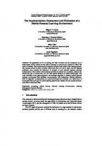
FIG. 2. LWC intercomparison data from periods A and F (Table 1) for the two PVMs. Regression statistics for 151 half-hour intervals: slope 5 1.000 6 0.003, R2 5 0.999, mean difference (GSI 2 OSU) 5 0.006 g m23, and std dev of difference 5 0.009 g m23. The 1:1 line is included for reference.

mean LWC values (at 10 m) ranged from 0.3 to 1.0 g m23 during persistent cloud; the 15-m value was typically 10% higher. Consequently, the sL/L threshold for steady cloud was decreased to 0.25 (dimensionless) so that ‘‘steady’’ cloud events represented the chosen conditions for investigating surface deposition (Vong and Kowalski 1995). a. Instrument intercomparisons 1) LWC

CALIBRATION

Data from periods A and F (refer to Table 1 for mounting configurations) were used to establish the calibration for the GSI PVM relative to the OSU PVM. For period F, some half-hour intervals with anomalously large droplets (as measured by the FSSP) were subjectively identified as outliers and removed from the intercomparison dataset. For these periods with extremely large droplets, the GSI PVM overestimated LWC by about 9% relative to the OSU PVM. The calibration of the GSI instrument therefore excluded data from period F where the droplet volume-weighted mean diameter (VMD) exceeded 18 mm. No droplet size data were available for period A but no outliers were in evidence. The result of this comparison (based on over 75 h of side-by-side, in-cloud operation) was that the GSI PVM had to be multiplied by a factor of 1.28 in order to achieve agreement with the OSU PVM. The offset of the instrument was not corrected; each instrument reported LWC relative to its measured ‘‘clear-air’’ signal for the offset as described previously. With the factor of 1.28 applied to the GSI PVM, the instrument agreement was excellent (R2 5 0.999, unity slope, negligible offset; Fig. 2). Both the standard deviation of the difference between the two instruments and the mean difference are less than 0.01 g m23.

474


2) PERIODS

VOLUME 14

OF POOR AGREEMENT

The PVMs showed some dependence of difference in measured LWC on their orientation with respect to the mean wind. For period B (Table 1), the GSI PVM overestimated LWC by about 0.025 g m23 for values of LWC ranging from 0 to 0.9 g m23. This small error is quite large relative to the excellent agreement demonstrated above. Another instance of relatively poor agreement in LWC was seen during period G (Table 1) when the GSI PVM overestimated LWC by approximately 0.08 g m23. Both of these periods of poor LWC agreement are marked by the GSI instrument sampling in the lee of an obstruction: during period B, the PVM sensing volume was downstream of its own receiver arm; during period G, the OSU PVM was located upstream of the GSI PVM. 3) PVM

FLUX COMPARISON

Data from periods C and D (Table 1) provided a unique perspective on the precision achievable with a PVM: a vertical gradient in LWC is detectable even with a separation of only 75 cm. Regardless of which instrument was where, the 10.75-m LWC was on average 0.04 g m23 larger than that measured at 10 m. This difference is four times the ‘‘normal’’ instrumental errors (above). Thus, given the imperfect sensor locations, these periods were not chosen for determining the calibration of the GSI instrument but are noteworthy in that a gradient in LWC can be detected over such a small change in height. For these periods, the comparison of surface-normal fluxes is presented in Fig. 3. Despite the vertical separation, the fluxes for the two instruments show very good agreement. In each case the rms difference is less than 2 mg m22 s21 for typical flux magnitudes of 7 mg m22 s21. Once again, the station bias (10 m versus 10.75 m) is consistent regardless of which instrument is where, and exceeds the random error. This suggests that the inability to perfectly collocate the instruments led to larger errors than the instruments themselves. The streamwise and transverse fluxes (u9L9 and v9L9, respectively, in the rotated coordinate system) show similar agreement. The rms difference in the streamwise flux was less than 2.3 mg m22 s21 for flux magnitudes typically ranging from 210 to 130 mg m22 s21 (R2 of 0.99 for the regression); the transverse flux had an rms difference of 3.6 mg m22 s21 for flux magnitudes typically ranging from 220 to 110 mg m22 s21 (R2 of 0.94). Although the instruments show good flux agreement, it is still worth examining their frequency response characteristics to ensure sufficient response times for flux characterization in the surface layer. Over 7 h (218 100-ms intervals) of in-cloud, side-by-side, 10-Hz PVM data from intercomparison period F have been decomposed into the frequency domain and are presented in Fig. 4 as squared-coherence and phase spectra (Black-

FIG. 3. Surface-normal LW flux intercomparisons for the PVMs during periods C (a) and D (b). Regression statistics: (a) for 46 halfhour intervals, slope 5 0.957 6 0.023, R2 5 0.975, mean difference (GSI 2 OSU) 5 -1.5 mg m22 s21, std dev of difference 5 1.3 mg m22 s21; (b) for 11 half-hour intervals, slope 5 0.937 6 0.017, R2 5 0.997, mean difference (GSI 2 OSU) 5 0.8 mg m22 s21, and std dev of difference 5 0.7 mg m22 s21. In each case, the 1:1 line is included for reference.

man and Tukey 1958), band-averaged to 100 degrees of freedom with the 95% significance level indicated. The two PVMs show near perfect coherence for frequencies below 0.1 Hz (perfectly in phase) and significant coherence even above 1 Hz. For the very highest frequencies (small-scale eddies), the 2-m transverse separation of the PVMs results in loss of correlation, but otherwise the instruments demonstrate a near-identical frequency response. The instruments are in-phase for frequencies up to 2 Hz. 4) FSSP–PVM

COMPARISON

The results for the FSSP–PVM intercomparison (period E) of LWC are shown in Fig. 5. These results are very similar to those previously reported by Vong and Kowalski (1995). Here too the standard deviation of the difference is greater than the mean difference, demonstrating no measurable bias between the two instruments. In the case of FSSP–PVM measurements, the

JUNE 1997

KOWALSKI ET AL.

475

FIG. 5. LWC intercomparison for the FSSP and OSU PVM. Regression statistics for 79 half-hour intervals: slope 5 1.011 6 0.015, R2 5 0.984, mean difference (FSSP 2 PVM) 5 0.023 g m23, and std dev of difference 5 0.035 g m23. The 1:1 line is included for reference.

FIG. 4. PVM spectral intercomparison: squared coherence and phase of the two PVMs for over 7 h of collocated data on 21 August.

bound for the measurement error in terms of the collocated difference is less than 0.035 g m23 for LWC values ranging from 0 to 1.0 g m23. The difference in the two LWC measurements showed no sensitivity to droplet size for VMDs ranging from 6 to 22 mm. Although the intercomparison period did not include any data with sufficiently high activity to cause the FSSP data to be flagged, there is evidence from default configuration data that errors can occur in the FSSP LWC that are related to activity. Figure 6 shows the 5-min LWC ‘‘error’’ (departure from the PVM LWC with 28-m lateral separation) for the FSSP plotted versus activity for a cloud event on 31 August. Clearly the difference between FSSP and PVM LWC is related to the activity and, thus, droplet number concentration. This difference in LWC is unrelated to the magnitude of the LWC. This relationship can be seen as well from default configuration data on a few other days with large droplet concentrations; the FSSP–PVM collocated intercomparison period lacked the high droplet number concentrations needed to demonstrate this type of LWC error. The activity correction employed here (Baumgardner 1983) is necessary for the good agreement in the FSSP and PVM intercomparison (i.e., removal of the correction degrades the LWC intercomparison) but apparently does not account for all of the coincidence and dead-time uncertainty associated with high activity in the FSSP. Furthermore, the results shown in Fig. 6 are not sensitive

to the exact value of the activity correction factor, as applied in (1), over the range of values suggested by other investigators (Baumgardner 1983; Baumgardner et al. 1985) and the manufacturer. This is consistent with the analysis of Brenguier (1989), which showed that the empirically derived activity correction is adequate only for low droplet number concentrations. In these data, the problem appears to be particularly pronounced (DLWC $ 0.1 g m23) for activity exceeding 35%, suggesting this value as a useful upper limit on this FSSP’s ability to sample clouds with high number concentrations (exceeding about 600 cm23). The FSSP and OSU PVM also agreed quite well for fluxes when collocated on the walk-up tower. Since the desired condition of steady cloud was rare during this intercomparison, all cloudy half-hour intervals from period E (see Table 1) were included; these data are likely

FIG. 6. LWC difference (FSSP minus PVM) vs FSSP activity; data from the default configuration on 31 August (FSSP and PVM are not collocated). Droplet number concentrations often exceeded 600 cm23 during this cloud event; more typical events during CACHE-3 had droplet concentrations near 200 cm23.

476


VOLUME 14

FIG. 7. Surface-normal LW flux intercomparison for the FSSP and OSU PVM. Regression statistics for 79 half-hour intervals: slope 5 1.072 6 0.040, R2 5 0.900, mean difference (FSSP 2 PVM) 5 -0.8 mg m22 s21, and std dev of difference 5 3.4 mg m22 s21. These data have not been subjected to the steady cloud criterion and therefore do not represent the chosen conditions for investigation of deposition to the surface. The 1:1 line is included for reference.

to contain periods of increased spatial inhomogeneity in the cloud and variable fluxes due to the influence of edge effects or entrainment. The results for surfacenormal fluxes are presented in Fig. 7. The standard deviation of the flux difference was again greater than the mean flux difference (no significant mean bias in the fluxes from the two instruments); this value bounding the instrumental error on the flux was less than 3.5 mg m22 s21 (for typical flux magnitudes of 6 mg m22 s21). For streamwise and transverse fluxes, the errors were somewhat larger (about four times as large, or similar to the flux magnitudes). Apparently the FSSP has an error that covaries with the strength of the horizontal winds, which is consistent with the hypothesis that ‘‘wind-ramming’’ affects the aspiration velocity and, hence, the effective sensing volume of the instrument (Fairall 1984; Choularton et al. 1986). Vong and Kowalski (1995) reported finding a signature for windramming in the streamwise LW flux, related to the streamwise variance of wind. Such a signal is not evident in these intercomparison data where the range of wind speeds at 10 m AGL (typically 4 m s21, and always less than 6 m s21) was low compared to the range encountered at the site. To demonstrate the degree of agreement between these two instruments in another way, time traces of LWC, sL/L, and LW flux for the first cloud event during this intercomparison (on 16 August, period E; see Table 1) are presented in Fig. 8. During periods of steady cloud with low sL/L, a downward flux of LW is measured; fluxes more variable in direction are noted during periods of larger sL/L. This is consistent with the findings of Vong and Kowalski (1995), who saw downward fluxes during periods of steady cloud when deposition was likely the dominant process in determining the flux. The

FIG. 8. Time traces of LWC, relative standard deviation of LWC (sL/L), and LW flux for 0400–1200 UTC 16 August, for the FSSP and the OSU PVM.

instruments show good agreement for LWC during this period, and reasonable agreement for LW flux. The frequency response of the FSSP and PVM also are analyzed with squared coherence and phase for seven hours of cloud (Fig. 9). Although not as good as for the PVM–PVM comparison, the FSSP and OSU PVM show very good coherence (versus near perfect) for frequencies below 0.1 Hz, with significant coherence (95% confidence) extending to above 0.5 Hz (instead of above 1 Hz as for the PVMs). These differences can be attributed to likely errors in the FSSP (discussed earlier) and to imperfect collocation of the instruments. The loss of phase also occurs at smaller frequencies than for the PVM–PVM case, probably because the instrument separation is partially streamwise rather than purely transverse to the flow due to the dimensions of the FSSP. Nevertheless, this result demonstrates very good agreement between the two instruments for frequencies that are relevant to flux calculation (0.001–1 Hz; Vong and Kowalski 1995). b. Sensitivity to coordinate rotations Each sonic anemometer produced a consistent relationship between the measured half-hour attack angle and wind direction, establishing the viability of rotation method 3. Figure 10 shows data from the default con-

JUNE 1997

477

KOWALSKI ET AL.

FIG. 9. FSSP–PVM spectral intercomparison: squared coherence and phase for over 7 h of collocated data collected on 17 August.

figuration that passed the screening criteria (section 3c). The solid line on the plot marks the mean attack angles for 58 intervals of wind direction and represents the empirical model used in method 3. Certain wind directions yielded greater variability in the attack angle, presumably due to the effects of a hillock on the slope (direction of approximately 2508 from the triangular tower, or 2558 from the walk-up tower) on airflow. The flux at the 15-m station showed very little sensitivity to the choice of methods 1 or 2 for coordinate rotation (i.e., using the 10-m or 15-m attack angle to rotate the 15-m flux). This uncertainty in the flux, based on choice of rotation scheme, can be characterized by a bias of 0.020 mg m22 s21 (slightly larger fluxes are computed using method 1) and a random error of 0.211 mg m22 s21, for 96 half-hour observations; these values are negligible relative to the instrument errors (section 4a). The fluxes and between-station flux differences showed little sensitivity to the choice of local-mean (method 1) versus wind direction (method 3) coordinate rotation schemes (results presented in Table 2). The bias, defined as the method 1 flux subtracted from the method 3 flux, is always less than 0.1 mg m22 s21 in magnitude. The random error is less than 1 mg m22 s21 in all cases. These errors are also negligible relative to the instrument errors presented above. Note that spatial differences in fluxes are less sensitive to choice of rotation method than are the fluxes themselves. The flux rotation

FIG. 10. Observed half-hour mean attack angle (points) and an empirical function (line) of wind direction for three sonic anemometers: 10-m walk-up tower (top panel), 10-m triangular tower (middle), and 15-m triangular tower (bottom).

method comparisons were not markedly worse for those wind directions that showed the greatest variability in attack angle (i.e., near 2508). 5. Discussion The two PVMs showed excellent agreement during CACHE-3 for all LWC intercomparisons except when the droplets were extremely large and/or when one instrument was sampling in a wake. Arends et al. (1992) reported that the PVM seemed less reliable for droplet TABLE 2. Sensitivities of the flux and flux difference to coordinate rotation methods 1 (local-mean coordinates) and 3 (wind direction coordinate system).

N (halfhours) 103 139 123 96 113

Flux (or flux difference) 10-m walk-up 10-m triangular 15-m triangular 10-m walk-up minus 10-m triangular 10-m triangular minus 15-m triangular

Bias [ method 3 minus Std dev of method 1 difference (mg m22 s21) (mg m22 s21) 20.020 20.057 0.098

0.963 0.722 0.386

0.074

0.692

0.048

0.447

478


VMDs larger than 20 mm. The measured error of 0.01 g m23 (2%–3% of typical mean LWC values during CACHE-3) from our most appropriate intercomparison dataset is small compared with differences in LWC over a mere 75-cm vertical separation. Regarding the wake effects on reported LWC, our hypothesis is that errors are introduced when an instrument is sampling in a turbulent wake in the lee of an obstruction, which may include its own arm when the PVM laser is parallel to the mean wind. This hypothesis is further supported by intercomparison data from period G where the GSI PVM was in the lee of the OSU PVM. Differences in LWC during this period often exceeded 0.1 g m23 and were correlated to the droplet size (VMD). This period was characterized by many 30-min intervals with VMDs greater than 20 mm; only this period and portions of period F (also with very large droplets) showed any sensitivity of the PVM agreement to droplet size. These periods of anomalously large droplets are not typical of cloud measurements at CPO; they introduce uncertainties that are not present in the vast majority of the data. When the droplet diameters were in the typical range of 10–18 mm for the site, the PVM agreement showed no sensitivity to droplet size. Of all the PVM intercomparison data, only data from periods B and G have shown other than excellent agreement in LWC and LW fluxes, with period G showing by far the worst agreement in the two instruments. These data had poor mounting configurations and, therefore, have been excluded from the intercomparison dataset. Exclusion of data from period G left periods C and D (Table 1) as the best configurations for PVM flux intercomparison. Despite the less than ideal configuration for flux intercomparison (75-cm vertical separation from the sonic anemometer for one PVM), the PVMs also showed excellent agreement with regard to LW fluxes. The error bound for surface-normal fluxes of about 2 mg m22 s21 is small compared with typical differences in fluxes between the 10-m and 15-m stations when the instruments are not collocated (data to be presented in a subsequent analysis). Furthermore, it was seen that this estimate is probably a conservative one since differences between the two ‘‘collocated’’ fluxes were shown to be dominated by a bias caused by the vertical separation. Streamwise and transverse flux agreement was slightly less ideal, but is less important to determination of forest interception of cloud droplets (McMillen 1988) and any associated environmental impacts. The FSSP–PVM intercomparison yielded results similar to those found during CACHE-1 (Vong and Kowalski 1995). 1) The instruments agreed very well for LWC without any need for wind-ramming corrections in the FSSP, 2) significant coherence extended to frequencies of nearly 1 Hz, 3) the surface-normal fluxes derived from covariances of LWC with winds from a collocated sonic anemometer also showed excellent agreement, and 4) the worst errors in flux for the FSSP are in the streamwise and transverse directions where

VOLUME 14

gustiness is most likely to have an effect on the aspiration velocity of the probe (Fairall 1984). The error estimates derived from this intercomparison are likely inflated due to the inclusion of ‘‘variable cloud’’ events (not meeting the steady criteria), which compounded the lack of perfect instrument collocation. Nevertheless, the excellent agreement displayed in Fig. 5 represents a result superior to previously published FSSP–LWC intercomparisons from both ground-based (Arends et al. 1992; Valente et al. 1989) and aircraft (Cerni 1983; Baumgardner 1983) sampling and suggests that LWC data from these two instruments (FSSP and OSU PVM) can be used interchangably. Measured point fluxes were found to be insensitive to the method of coordinate rotation. This is particularly true for flux differences between separated measurement stations. The small differences between methods represent uncertainties in the flux based on uncertainties in the direction in which the flux ought to be measured and do not necessarily represent errors that are additive to the estimated instrumental errors [sections 4a(3) and 4a(4)]. Nevertheless, were one to sum squared errors from instrumental and methodological sources, the methodological errors would be negligible. No conclusions are drawn about the superiority of any of the rotation techniques; the differences between them are negligible with regard to determination of fluxes and flux differences at different locations. The demonstration of precision in these measurements of LWC and LW flux was dependent upon exhaustive instrument intercomparison. This is particularly true for the GSI PVM, which showed excellent agreement with the other instruments, but only after a calibration correction. The error bounds established here will allow determination of both LW gradients and the LW flux divergence from spatially separated instruments. More definitive studies of forest uptake by occult deposition, beyond the capabilities of current technology, would include measurement of in-cloud water vapor densities and fluxes, allowing closure of the total water budget. 6. Conclusions LWC and LW flux intercomparison studies have been performed to place bounds on errors between three microphysical instruments when making nearly collocated measurements. In each case, the OSU PVM has been considered the standard against which the other two microphysical instruments have been compared. A calibration factor for the GSI PVM has been established based on the ‘‘best’’ collocated data for the two PVMs. The error for LWC measured by a PVM has been found to be less than 0.01 g m23 with the error bound for the PVM-based surface-normal LW flux of less than 2 mg m22 s21. The PVMs exhibited some sensitivity to droplet size in their agreement, but only for anomalously large droplets (VMD . 18 mm). For the FSSP, the error

JUNE 1997

KOWALSKI ET AL.

for LWC was found to be less than 0.035 g m23 with an estimated LW flux error of less than 3.5 mg m22 s21; larger FSSP-based LW flux errors are possible at higher wind speeds when wind ramming can be important. Errors in the FSSP LWC were seen to be related to ‘‘activity’’ when droplet concentrations exceed 600 cm23; this FSSP appears to overestimate the LWC when activity exceeds 35%. The above error bounds are conservative in that they include the effects of imperfect collocation of instruments, particularly in the case of the FSSP–PVM intercomparison. Three methods of rotating coordinate systems based on mean winds have been analyzed and seen to be negligibly different. A maximum uncertainty (error) of 1 mg m22 s21 in the surface-normal LW flux was found based on uncertainty in the direction of rotation, but a smaller value (at most, about 0.7 mg m22 s21) is relevant to interpreting differences in fluxes between different stations. These bounds on instrumental and methodological errors in determining LW fluxes should be very useful for interpreting such measurements and characterizing the processes that govern occult deposition. Acknowledgments. Special thanks go to Dr. David Covert for the use of his site, tower, and facilities and for all of his help with setting up the CACHE projects. Thanks are also due to the entire ASTER crew: Tom Horst, Kurt Knudson, Charlie Martin, John Militzer, Santiago Newbery, Steve Oncley, Steve Semmer, and Lou Verstraete. This work was supported by National Science Foundation Grant ATM9118316 (Atmospheric Chemistry desk). The 5-min mean and covariance data described in section 2b have been reprocessed and are available via anonymous FTP from ftp://stout.atd.ucar.edu/pub/ cache/aster. Contact Andrew Kowalski (andyk@ ats.orst.edu) or Gordon Maclean ([email protected]) for more information. REFERENCES Arends, B. G., G. P. A. Kos, W. Wobrock, D. Schell, K. J. Noone, S. Fuzzi, and S. Pahl, 1992: Comparison of techniques for measurements of fog liquid water content. Tellus, 44B, 604–611. Baumgardner, D., 1983: An analysis and comparison of five water droplet measuring instruments. J. Climate Appl. Meteor., 22, 891–910. , W. Strapp, and J. E. Dye, 1985: Evaluation of the forward scattering spectrometer probe. Part II: Corrections for coincidence and deadtime losses. J. Atmos. Oceanic Technol., 2, 626–632. Beswick, K. M., K. Hargreaves, M. W. Gallagher, T. W. Choularton, and D. Fowler, 1991: Size-resolved measurements of cloud droplet deposition velocity to a forest canopy using an eddy correlation technique. Quart. J. Roy. Meteor. Soc., 117, 623–645. Blackman, R. B., and J. W. Tukey, 1958: The Measurement of Power Spectra. Dover, 178 pp. Brenguier, J. L., 1989: Coincidence and dead-time corrections for particle counters. Part II: High concentration measurements with an FSSP. J. Atmos. Oceanic Technol., 6, 585–598. Businger, J. A., and A. C. Delany, 1990: Chemical sensor resolution required for measuring surface fluxes by three common micrometeorological techniques. J. Atmos. Chem., 10, 399–410.

479

Cerni, T. A., 1983: Determination of the size and concentration of cloud drops with an FSSP. J. Climate Appl. Meteor., 22, 1346–1355. Choularton, T. W., D. Consterdine, I. Gardner, B. Gay, M. Hill, J. Latham, and I. Stromberg, 1986: Field studies of the optical and microphysical characteristics of clouds enveloping Great Dun Fell. Quart. J. Roy. Meteor. Soc., 112, 131–148. Dabberdt, W. F., and T. W. Schlatter, 1996: Research opportunities from emerging atmospheric observing and modeling capabilities. Bull. Amer. Meteor. Soc., 77, 305–323. , D. Lenschow, T. Horst, P. Zimmerman, S. Oncley, and A. C. Delany, 1993: Atmospheric surface exchange measurements. Science, 260, 1472–1480. Dye, J. E., and D. Baumgardner, 1984: Evaluation of the forward scattering spectrometer probe. Part I: Electronic and optical studies. J. Atmos. Oceanic Technol., 1, 329–344. Fairall, C. W., 1994: Interpretation of eddy correlation measurements of particulate deposition and aerosol flux. Atmos. Environ., 18, 1329–1337. Fuzzi, S., 1994: The Kleiner Feldberg cloud experiment 1990: Introduction. J. Atmos. Chem., 19, 1–2. , and Coauthors, 1992: The Po Valley Fog Experiment 1989: An overview. Tellus, 44B, 448–468. Gerber, H., 1991: Direct measurement of suspended particulate volume concentration and far infrared extinction coefficient with a laser diffraction instrument. Appl. Opt., 30, 4824. Heintzenberg, J., 1992: The Po Valley Fog Experiment 1989: What have we learned, where do we go from here? Tellus, 44B, 443–447. Højstrup, J., 1993: A statistical data screening procedure. Meas. Sci. Technol., 4, 153–157. Kaimal, J. C., J. E. Gaynor, H. A. Zimmerman, and G. A. Zimmerman, 1990: Minimizing flow distortion errors in a sonic anemometer. Bound.-Layer Meteor., 53, 103–115. Knollenberg, R. G., 1981: Techniques for probing cloud microstructure. Clouds, Their Formation, Optical Properties, and Effects, P. V. Hobbs and A. Deepak, Eds., Academic, 15–91. Lovett, G. M., and J. D. Kinsman, 1990: Atmospheric pollutant deposition to high-elevation ecosystems. Atmos. Environ., 24A, 2767–2786. McMillen, R. T., 1988: An eddy correlation technique with extended applicability to non-simple terrain. Bound.-Layer Meteor., 43, 231–245. Miller, E. K., A. Friedland, E. Arons, V. A. Mohnen, J. Battle, J. A. Panek, J. Kadlecek, and A. H. Johnson, 1993: Atmospheric deposition to forests along an elevational gradient at Whiteface Mountain, NY, USA. Atmos. Environ., 27A, 2121–2136. Rogers, R. R., and M. K. Yau, 1989: A Short Course in Cloud Physics, Pergammon, 293 pp. Schuepp, P. H., M. Y. Leclerc, J. I. MacPherson, and R. L. Desjardins, 1990: Footprint prediction of scalar fluxes from analytical solutions of the diffusion equation. Bound.-Layer Meteor., 50, 355–373. Valente, R. J., R. K. A. M. Mallant, S. E. McLaren, R. S. Schemenauer, and R. E. Stogner, 1989: Field intercomparison of groundbased cloud physics instruments at Whitetop Mountain, Virginia. J. Atmos. Oceanic Technol., 6, 396–406. Vong, R. J., and A. S. Kowalski, 1995: Eddy correlation measurements of size-dependent cloud droplet turbulent fluxes to complex terrain. Tellus, 47B, 331–352. , H. C. Hansson, H. B. Ross, D. S. Covert, and R. J. Charlson, 1988: Northeastern Pacific sub-micrometer aerosol and rainwater composition: A multivariate analysis. J. Geophys. Res., 93(D2), 1625–1637. Wesely, M. L, 1970: Eddy correlation measurements in the atmospheric surface layer over agricultural crops. Ph.D. dissertation, University of Wisconsin—Madison, 102 pp. Wyngaard, J. C., 1981: The effects of probe-induced flow distortion on atmospheric turbulence measurements. J. Appl. Meteor., 20, 784–794. , and S. F. Zhang, 1985: Transducer shadow effects on turbulence spectra measured by sonic anemometers. J. Atmos. Oceanic Technol., 2, 548–558.