Proceedings of the 46th IEEE Conference on Decision and Control New Orleans, LA, USA, Dec. 12-14, 2007
FrB05.2
Design and Tuning of Standard Additive Model Based Fuzzy PID Controllers for Multi-Variable Process Systems Eranda Harinath and George K. I. Mann
Abstract—This paper describes a two-level tuning method for fuzzy PID controllers for multi-variable control system. The fuzzy PID system is designed using the inference of Standard Additive Model (SAM). In the two-level tuning scheme the tuning follows two steps, low-level tuning followed by high-level tuning. The low-level tuning adjust the linear gain parameters. The high-level tuning changes the nonlinearity in the normalized fuzzy output. For that purpose a nonlinearity diagram is defined to choose membership parameters of the fuzzy system. The controller performance is verified through real-time multi-zone soil temperature control problem having a 3 × 3 process system. The proposed method can be used for any n × n dimensional multi-input-multi-output (MIMO) process system. Index Terms—FPID control, standard additive model, multivariable control, linear PID tuning, static de-coupler
I. INTRODUCTION The main challenge in fuzzy logic control (FLC) design is in the tuning, particularly in choosing correct fuzzy system and its associated fuzzy parameters. The curse of dimensionality during the rule explosion [1] has been the main drawback in FLC designs. In a typical Fuzzy Proportional Integral Derivative (FPID) design problem the tuning parameters includes linear scaling parameters of the control variables, fuzzy membership parameters, rules and other associated fuzzy variables in the rules base, such as number of rules, membership distribution and rule composition. The mathematical complexity in the nonlinear fuzzy control makes the formulation of a tuning mechanism an extremely a complex problem. However, the recent increase in computing power enabled most designers to adopt numerical optimization techniques for generating optimum or near optimum solutions to fuzzy systems, such as genetic algorithm and neural network, where those techniques have the capacity to determine a large number of unknown parameters in fuzzy systems [2]. However, those application are somewhat specific and unable to generalize for wider process specifications. Most of those designs adopt off-line optimization methods and cannot be implemented for online control. Moreover the optimizations requires an accurate process model and any process mismatch This work was undertaken as a part of PPSC (Pan-Atlantic petroleum system consortium) project funded from Atlantic Innovation fund and Financial assistance from Natural Sciences and Engineering Research Council (NSERC) of Canada is gratefully acknowledged E. Harinath is with Department of Electrical and Computer Engineering, University of British Columbia, Vancouver, BC, V6T 1Z4, Canada
[email protected]
G. K. I. Mann is with the Faculty of Engineering and Applied science, Memorial University of Newfoundland, St. John’s, NL, A1B 3X5, Canada
[email protected]
1-4244-1498-9/07/$25.00 ©2007 IEEE.
during operation can result in poor stability and affect the overall performance. There is a huge volume of FPID applications available in the literature where the control has been performed for variety of processes, including nonlinear systems. Almost all of these applications belong to Single-Input Single-Output (SISO) process systems. Only in a very few applications the Multi-Input Multi-Output (MIMO) systems have been considered. Chieh and Pey [3] used pre-compensator to decouple the MIMO process and the design is based on RosenbrockNyquist Array (RNA) method. However, the FPID parameters have been chosen arbitrary. Gamero and Medrano [4] used Mamadani based FPID to control a biotechnology process. They have used dynamic de-coupler in order to reduce loop interactions. The controller is based on a two- dimensional Mamdani type fuzzy rule base. The application of dynamic de-coupler for multi-variable process is sometimes not physically realizable [5]. Dynamic de-coupler is also shown to be more sensitive to plant and process mismatch and therefore is less popular in process control. In another application, Rahmati et. al. [6] used fuzzy PID controller for HVAC plant. They have presented similarity between conventional digital PID control algorithm and Takagi-Sugeno based fuzzy PID control. Recently, Shaoyuan et. al. [7] presented coordinated control strategy for boiler- turbine control using fuzzy reasoning and auto-tuning techniques. Self-organizing FPID controller is presented by Hassan et. al. [8] for robot arm. In these applications fuzzy logic controllers are used at supervisory level for self tuning of conventional PID gains at the lower level. In all aforementioned methods the design and tuning of FPID have been arbitrary and the gain parameters were chosen using trial and error methods. The literature review revealed that there is no systematic design procedure is available to design and tune FPID controllers for MIMO process systems. It is very clear that the available SISO based FPID design techniques have limitations to extend for general MIMO systems. Alternatively, this paper proposes a generalized tuning scheme for both linear PID and FPID controllers. The FPID controller follows the fuzzy inference based on Standard Additive Model (SAM), proposed in [1]. The proposed tuning scheme follows two levels of tuning, namely low-level tuning followed by highlevel tuning [9]. By considering interaction measure among loops a generalized tuning technique is developed for lowlevel tuning for MIMO process. In SAM based fuzzy inference the consequent fuzzy sets are weighted using either centroid or volume of membership functions which can also
5306
46th IEEE CDC, New Orleans, USA, Dec. 12-14, 2007
FrB05.2
ûf
be calculated in advance using SAM theorem. In the proposed design the high-level tuning is dedicated to determine these centroid and volumes in the view of achieving desired nonlinearity of the fuzzy output.
ûf 1
(θ1)1i
(θ1)wi
(θ1)2i
1
(α1)wi
0 0 (α0)wi -1 1 ê2i
II. TWO-LEVEL TUNING
0
(θ0)2i
(θ0)1i
1 ê1i (θ0)wi
0
-1 -1
The FPID design can be classified as a two-level tuning problem [9] in which the tuning process is decomposed into two tuning levels. While low-level tuning addresses the linear gain and overall stability, the high-level tuning provides nonlinear control to enable superior performance. In a rulecoupled fuzzy system, such as Mamdani-Zadeh based system, the inputs (error and its derivative) are coupled to produce a combined FPI output [9]. The coupled nature of the inputs generally makes the nonlinear output a complex function. As a result, it is difficult for one to isolate linear gains from the nonlinear output. In order to facilitate the two-level tuning, we define apparent linear gains (ALG) and apparent nonlinear gains (ANG). While the ALG terms are related to the overall performance and stability of the system the ANG terms provide the nonlinearity that is necessary in the fuzzy output. In the past for SISO systems, some have attempted to provide tuning rules for linear gains [10]. However the nonlinear tuning was not sufficiently or explicitly described. In [11], the design of a conventional FPID is identified as a two-level tuning problem and described as a way of obtaining ALG terms for conventional FPID type controllers. However, the non-linearity tuning was not sufficiently or explicitly described for implementing a two-level tuning. In following sections a systematic procedure is developed to devise twolevel tuning methodology for general FPID controllers for MIMO systems. A. Fuzzy PID (FPID) Configurations ei ∆ei ∆2ei
Sei Scei Srcei
êi ∆êi
∆ûPIDi +
F (êi,∆êi,∆2êi)
uPIDi
ûPIDi
SAM
Su + Z-1
∆2êi
(a) SAM
êi
SAM
F2(êi)
û2i KIiTs
uPIDi
ûPIDi Su
+ +
Z-1 SAM
+
û3i KDi/Ts
F3(êi)
1
0
ê
(b)
Fig. 2. Nonlinear tuning variables measured at local control points for FPID configurations
PID signal [12]. Using suitable scale factors (Swi ),where w = 1, 2, 3, the feed back error terms (ei ) and its corresponding normalized error variables (eˆi ) at nth sampling instance can be expressed as eˆi (n) = S1i ei (n), ∆eˆi (n) = S2i ∆ei (n), ∆2 eˆi (n) = S3i ∆2 ei (n). All FLC input variables are normalized to a compact region [-1,1]. The error variables are normalized by using the condition eˆwi = max(−1, min(1, Swi ewi )). The defuzzified controller output after the fuzzy inference is denoted by u. ˆ Similarly the FLC output is normalized by using the condition uˆ ≡ u/umax . 1) High-Level Nonlinear Tuning Variables: The nonlinear tuning variables are selected to affect ANG terms at any given local control point in the control surface. Since PID gains are proportional to the slopes of the control surface, the slope angles of the tangents drawn at a given point on the nonlinear control surface are considered to be the nonlinear tuning variables. For simplicity, two slope angles drawn at two selected points (see Fig. 2) on control surface are considered as nonlinear tuning variables. In order to isolate slope angles from their associated outputs of FPID type I controller, the slopes are measured in the planes of individual error axes. The measurement of these angles with respect to a two-dimensional control surface is shown in Fig. 2(a). Fig. 2(b) shows a control curve that has been projected into a chosen error variable. In general, for a threeinput coupled can ´ base the slope angles ´ be described by ³ rule ³ ∂ uˆ ∂ uˆ , (θ1 )wi = ∂ eˆwif where uˆ f = (θ0 )wi = ∂ eˆwif eˆwi =1
u( ˆ eˆ p = 0), p = 1, 2, 3 p 6= w. The fuzzy system designed for the PID control should allow independent variations of θ0 and θ1 within the range [0 90◦ ]. 2) Low-Level Linear Tuning Variables: The composed FPID control action for FPID type I is given by
KPi
+
(a)
eˆwi =−1
û1i
F1(êi)
Sei
-1
Z-1
n
(b)
uPIDi = Sui ∑ ∆uˆPIDi .
Fig. 1. FPID configurations. (a) Type I: rule-coupled FPID, (b) Type II: rule de-coupled FPID
Two types of FPID configurations are considered as shown in Fig.1. The type I is a conventional Mamdani’s type FPID and has three inputs and it produces an incremental FPID signal. The type II uses SISO rule inference to provide decoupled and independent tuning for the three actions in the
(1)
k=0
Assuming the fuzzy integral action and derivative actions are in the form given by, uˆI (n) = ∑nk=0 uˆw (k) and uˆD (n) = uˆw (n)− uˆw (n − 1), the FPID action for FPID type II can be expressed as uPIDi = Sui [KPi uˆ1i + KIi Ts ∑nk=0 uˆ2i (k)+ (2) KDi Ts (uˆ3i (n) − uˆ3i (n − 1))]
5307
46th IEEE CDC, New Orleans, USA, Dec. 12-14, 2007
Decentralized fuzzy or linear PID
Static Decoupler
MIMO Process
r +
D
Gc
-
G
FrB05.2
Where it is assumed that G(0) is non-singular. The PID controller matrix in a n × n MIMO process is expressed as,
y
Gc (s) = diag{c1 (s), . . . , cn (s)}. Fig. 3.
Statically de-coupled multi-variable control
where KPi , KIi and KDi are the linear PID gains for ith loop and Ts is the sampling time. When a fuzzy system is set to produce a linear function, the FLC will become a linear type PID controller and is defined as an equivalent linear controller (ELC) [13]. Using the ELC output the ith loop linear PID output can be arranged in the following form; n
ulPIDi (n) = KPai ei (n) + KIai ∑ ei (k)Ts + KDai ∆ei (n)/Ts
(3)
k=0
where KPai , KIai and KDai are defined as the ALG terms of the FLC system. A FLC having linear rule base and uniform partition of universe of discourse of all variables is named as a linear-like fuzzy logic controller (LLFLC) [13]. The ELC defined for the LLFLC is used for deriving the linear tuning variables. Then the ELC output for type I is given by ∆uˆlPIDi = [eˆi + ∆eˆi + ∆2 eˆi ].
(4)
From (3) and (4), the ALG terms can be found as KPai = Su S2i KIai = Su S1i /Ts and KDai = Su S3i Ts . Similarly, ELC output for type II is given by uˆl1i = uˆl2i = uˆl3i = eˆi .
(5)
From (3) and (5), the ALG terms can be found as KPai = K pi , KIai = KIi and KDai = KDi . The gain analysis provides two tuning control. The adjustment of KPa , KDa and KIa refers to a general PID tuning with the control surface normalized to a linear form in the normalized output space. The ANG terms refers the effect of changing the nonlinearity of the FPID output in the nonlinearity output space. This ALG and ANG decomposition allows the use two level of tuning for fuzzy PID controllers. III. LOW-LEVEL TUNING: LINEAR PID CONTROLLER TUNING
L(s) = G(s)D(s).
(9)
Where G is the MIMO process modeled assuming an openloop stable first-order plus dead time model and D is the static de-coupler. Using the truncated Taylor series expansion, the above transfer function L is approximated to a firstorder model. Since higher order terms in the Taylor series expansion are made to zero, this approximation is valid only at low frequencies. The approximated system is thus given by, L(s) ≈ [li j ] . (10) 1 . Tii represents Where li j = Ki j s ; i 6= j and lii = Tii s+1 th the time constant of the i SISO loop and Ki j ; i 6= j represents off diagonal parameters which represent different loop interactions during steady state. It is clear that at low frequencies the off-diagonal terms are proportional to the frequency (s). Hence the system can be approximately decoupled if the bandwidth of decentralized PID controllers are low enough. The open-loop transfer function of the system shown in Fig. 3 is written as Q(s) = G(s)DGc (s) = L(s)Gc (s). Let Q(s) = [qi j ] . (11)
Where qi j = Ki j s(KPi + K KPi + sIi +KDi s Tii s+1
KIi s
+ KDi s)
;
i 6= j and qii =
. The close-loop relation for this system is expressed as y = [I + QGc ]−1 QGc r where r and y are input and output vectors respectively. Then, the closed transfer matrix H(s) between y and r can be written as, H(s) = [I + Q(s)Gc (s)]−1 Q(s)Gc (s). (12)
B. Tuning jth Loop
The conventional feedback strategy of a n inputs n outputs multi-variable system with a static de-coupler and a FPID controller is shown in Fig. 3 where the multi-variable system is assumed as a linear and open-loop stable system. Then, the transfer function of this MIMO process system is denoted by, (6)
The open-loop SISO transfer function between ith output and jth input when all other inputs are zero is denoted by gi j where i, j = 1, 2, . . . , n. The static de-coupler D for the above system can be described using (7). D = G−1 (0)
Where ci (s) = KPi + KsIi + KDi s and KPi , KIi and KDi are proportional, integral and derivative gains of the ith PID controller. For the above system, shown in Fig. 3, the overall compensated system i.e. process model and static de-coupler can be written as,
H(s) = [hi j ] .
A. System Description
G(s) = [gi j ] .
(8)
When all other loops are open, the elements in jth column q (s) of H(s) can be written as, hi j (s) = 1+qi j j j (s) = qi j (s)S j where S j = (1 + q j j (s))−1 is defined as sensitivity function of the jth loop [14]. Thus, for a step input change in the jth loop, the interactions to other loops at low frequencies can be computed as, hi j (s) =
lim qi j (s)S j
s→0
= Ki j KI j S j .
(13)
Then the upper bound of interaction is given by,
(7)
5308
| hi j (s) | ≤ max(| Ki j |) | KI j | (S j )max i6= j
(14)
46th IEEE CDC, New Orleans, USA, Dec. 12-14, 2007
FrB05.2
where (S j )max is the maximum value of S j and max(| Ki j |) is the maximum absolute value of Ki j ; i 6= j. Hence we can introduce interaction index of the jth loop as, I j = max(| Ki j |) | KI j | (S j )max .
y
B5 B4
(15)
i6= j
B3 B2
The value of KI j can be calculated at particular value of (S j )max so that the interaction index, I j is kept as low as possible. Then, the rest of interactions can also be reduced according to the inequality (14). The proportional gain, KP j of PID controller is computed using time constant of the firstorder approximated process and the designed integral gain. The derivative gain, KD j is chosen from ZN formula as,
B1 A1
KD j =
4KI j
Fig. 4.
KD j s2 +KP j s+KI j T j j +KD j 1+KP j KI j 2 s + ( T j j +KD j )s + T j +K Dj
A4
A5
Function approximator: Additive fuzzy system B'0
If A1 then B1
B'1
If Am then Bm
w0 w1 B
...
A
If A0 then B0
B'm
Centroidal Defuzzifier
y = F(x)
wm
General framework of additive fuzzy system
(17)
In order to find KP j , In this analysis we use direct pole placement method [14] as follows. The closed loop transfer function of the jth loop with reduced first-order model and PID controller is given by, h j j (s) =
x
Fig. 5.
.
A3
x
1 TD j = TI j . (16) 4 Where TD j and TI j are derivative and integral time constants for PID controller at the jth loop. Then, KP2 j
A2
.
(18)
Considering second-order dynamics of the numerator in (18), the cross q over frequency of the first loop can be written as, ωo j = KI j /(T j j + KD j ) and the proportional gain is given by, (19) KP j = 2ζ j ωo j (T j j + KD j ) − 1.
a fuzzy inference mechanism is quite important in achieving efficient high-level tuning [12]. It is found that SAM based fuzzy inference has the capacity to provide better nonlinearity tuning as opposed to traditional min-max-gravity inference [15]. SAM is a special case of the additive model framework (see Fig. 4 and Fig. 5) and following can be observed as special properties in SAM. 1) The fired then-part set B0β is the fit product aβ (x)Bβ . Where the fit value aβ (x) (aβ is called membership function) express the membership grade of input x in the if-part fuzzy set Aα . Then the output set can be expressed as, m
B=
Where ζ1 is the damping constant of a second-order system. From (17) and (19), q 1 ± ζ j KI2j − 4ζ j2 KI3j T j j + 4KI j T j2j . (20) KP j = 4KI2j ζ j2 − 1 The same procedure is repeated for other loops and tuned while keeping interaction index as minimum. IV. HIGH-LEVEL TUNING : NONLINEARITY TUNING The high-level tuning is dedicated to determine fuzzy rule base parameters which has direct relevance to the nonlinearity of the FLC output. The nonlinearity that is generated through fuzzy mapping is then adjusted using highlevel tuning parameters. In general the nonlinearity can be adjusted either by changing rules or by changing knowledge base rule parameters, such as membership shapes and their distributions in the universe of discourse of variables. An effective nonlinearity tuning mechanism should have the capacity to produce a flexibility to change the nonlinearity of the fuzzy output in a wider range. A proper selection of
∑ wβ aβ (x)Bβ (x).
(21)
β =1
2) The system output F(x) computes as centroid of output set B(x) and defuzzifies to a scalar or a vector. ! Ã m
F(x) = Centroid
∑ wβ aβ (x)Bβ (x)
(22)
β =1
The centroid provides the structure of a conditional expectation to the fuzzy system F and it acts as an optimal nonlinear approximator in the mean-squared sense. V. DESIGN OF SAM FOR FPID CONFIGURATIONS A. Rule-coupled Fig. 6 shows the SAM representation of rule-coupled (FPID type I) for three-inputs single-output system. In this design we have selected membership functions (ai ) for the if-part in SAM as triangle functions as shown in the Fig. 7. With the min combiner, the SAM output for the above system can be written as,
5309
F(x) =
∑βm=1 wβ min{aβ (x1 ), aβ (x2 ), aβ (x3 )}Vβ Cβ . ∑m β =1 wβ min{aβ (x1 ), aβ (x2 ), aβ (x3 )}Vβ
(23)
46th IEEE CDC, New Orleans, USA, Dec. 12-14, 2007
FrB05.2
Output Temperature Rise PID 740 730 700
y1 y2 y3
Set Point Tracking Overshoot % PID FPID1 FPID2 16.7 10.0 11.7 10.0 9.0 3.0 17.7 11.7 15.8
Time (minute) FPID1 FPID2 1700 445 1080 260 1590 425
TABLE I P ERFORMANCE CHARACTERISTIC INDICES OF PROPOSED FPID METHODS AND PID Loop No
PID
FPID1 P
I ×10−5 2.5 1.4 2.4
P 0.16 0.18 0.15
(1) (2) (3)
D ×10−6 9.5 8.4 9.5
v1 0.5 0.9 0.6
v3 0.8 1.0 1.0
v1 1.8 3.1 2.3
v3 1.5 1.1 0.9
Setting Time (minute) PID FPID1 FPID2 2300 3670 1000 3750 2500 960 2050 3550 1000 METHOD FOR SET POINT TRACKING
FPID2 I v1 v3 2.5 1.8 2.6 1.1 1.9 1.2
D v1 2.1 3.9 1.8
v3 1.3 0.9 1.2
TABLE II T UNING PARAMETERS OF FPID AND PID CONTROLLERS FOR REAL TIME EXPERIMENTS
If A0 and D0 and E0 then B0 x2
If A1 and D1 and E1 then B1
w0 B'1
w1 y = F(x)
wm B'm
If Am and Dm and Em then Bm
Fig. 6.
Centroidal Defuzzifier
B
...
x3
In this analysis, the then-part centroid Cwi are selected as, C0i = −1, C1i = 0 and C2i = 1. The stability properties are determined by the extreme values of equivalent PID gains. Therefore, to guarantee stability, the maximum and minimum ANG terms are considered in an equivalent linear PID system. In the SAM inference the maximum or minimum of ANG occurs when eˆi = −1, eˆi = 0 and eˆi = 1. Then, the slope angle at selected four points (see Fig. 2) are,
B'0
x1
SAM representation of rule-coupled fuzzy system A0i , (V0i)
A1i , (V1i)
A2i , (V2i)
1
-1
Fig. 7.
0
1
êw
Membership functions for if-part in SAM
Since each rule uses one (min of fired membership values) of the three-inputs to de-fuzzyfy, it is equivalent to a SISO SAM system. In other word the analysis of rule-coupled FPID configuration in the view of SAM is similar to rule de-coupled FPID configuration. B. Rule de-coupled Consider two control regions in the controller output space. The first region is when the normalized error variables are −1 ≤ eˆi < 0. The local control in this region affects steady state, load disturbance and overshoot properties. The second region is when 0 ≤ eˆi ≤ 1. The control in this region affects the speed of response during the transient, undershoot and steady state properties. The objective is to realize independent adjustment of FLC parameters in the view of changing ANG terms at the chosen control points. The slope angle θ for type II (see Fig. 2(b)) can be described by, ³ ´ V0i (2eˆiV0iC0i −2C0iV1i eˆi −C0iV1i +V1iC1i ) arctan (eˆiV0i −eˆiV1i −V1i )2 for³ − 1 ≤ eˆi < 0 ´ (24) θ= V2iV1i (−C2i +C1i ) arctan − (V 2 1i eˆi −V1i −V2i eˆi ) for 0 ≤ eˆi ≤ 1
(θ0 )wi = arctan(V1i /V0i ) , (α0 )wi = arctan(V0i /V1i )
(25)
(θ1 )wi = arctan(V1i /V2i ) , (α1 )wi = arctan(V2i /V1i )
(26)
It is clear, the pairs {(θ0 )wi , (α0 )wi } and {(θ1 )wi , (α1 )wi } form a right angle. There are two independent slope angles that can be defined over the control surface of SAM corresponding to two regions −1 ≤ eˆi < 0 and 0 ≤ eˆi ≤ 1. Therefore we select (θ0 )wi and (θ1 )wi as the two independent slope angles to be adjusted within the range of [0 − 900 ] for high-level tuning. In order to find two independent angles, the then-part volume for second membership function is selected as unity:V1i = 1. Then, (27) θ0 = arctan(1/V0 ) , θ1 = arctan(1/V2 ). Hence the terms V0 and V2 are the nonlinear tuning variable for the SAM. VI. REAL TIME EXPERIMENTS The objective of experiments is to control temperatures at three different locations of soil-cell using three different heaters. The experimental set-up is shown in Fig.8. The system identification is performed for soil-cell via classical step response method. Open loop tests (step response) are carried out for soil- cell and transfer function matrix found as, 5e−487s 13.42e−54s 0 168s+1 397.5s+1 −184s 19.8e−99s 4.1e−271s . (28) G(s) = 3.019e 258s+1 462s+1 313.5s+1 0
2.25e−553s 358.5s+1
12.5e−55.5s 178.5s+1
Three different type of control algorithms; PID, FPID type I and FPID type II are implemented for soil-cell. The room
5310
46th IEEE CDC, New Orleans, USA, Dec. 12-14, 2007
FrB05.2
System response, y1
36
34
dSPACE Controller Board Soil Cell
32 Temperature 0C
Signal Conditioner
30
28
26 Power Suplliers
PID FPID type 1 FPID type 11
24 PC
22
Fig. 8.
0
1000
2000
Experimental set-up for soil-cell
3000
4000 5000 time (minute)
6000
7000
8000
6000
7000
8000
6000
7000
8000
(a) g12 System response ,y2
44
temperature was around 22o C for all experiments. The initial set point temperature for loop 1 and 3 was 28o C and for loop 2 was 32o C. After the all outputs reached their set point values, the set point temperatures were changed 34o C for loop 1 and 3, and 42o C for loop 3 at 4000 min respectively. The Fig. 9 shows responses of each system.
42 40
Temperature 0C
38 36 34 32 30 28
VII. CONCLUSIONS
26
The design of an FPID here is treated as a two-level tuning problem. A novel linear and nonlinear tuning methodology has been formulated based on two-level tuning method. As opposed to general Mamdani-Zadeh type configuration, SAM based fuzzy inference is implemented to achieve better nonlinearity in the fuzzy output. The results show improved performance of the proposed FPID system against the linear PID system.
24 22
1000
2000
3000
4000 5000 time (minute)
(b) g22 System response, y3
36
34
Temperature 0C
32
R EFERENCES [1] Bart Kosko. Fuzzy Engineering. Prentice-Hall, Inc, Simon and Schuster/A Viacom Company Upper Saddle RIver, New Jersey, 1997. [2] Yu Yongquan, Huang Ying, Wang Minghui, Zeng Bi, and Zhong Guokun;. Fuzzy neural pid controller and ftuning its weight factors using genetic algorithm based on different location crossover. Systems, Man and Cybernetics, 2004 IEEE International Conference on, 4:3709–3713, 10-13 Oct. 2004. [3] Chieh-Li Chen and Pey-CHung Chen. Application of fuzzy logic controllers in single-loop tuning of multivariable system design. Computers in Industry, 17(1):33–41, 1991. [4] Eduardo G. I and Hiram M. R. Fuzzy multivariable control of a class of a biotechnology process. Proceedings of the IEEE International Symposium on Industrial Electronics, 1:419–424, July 1999. [5] B. Wayne Bequette. Process Control Modeling, Design and Simulation. Prentice -Hall of India, 2003. [6] Rahmati A, Rashidi F, and Rashidi M. A hybrid fuzzy logic and pid controller for control of nonlinear hvac systems. IEEE Transactions on Systems, Man and Cybernetics, 3:2249–2254, October 2003. [7] Shaoyuan Li, Hongbo Liu, Wen-Jian Cai, Yeng-Chai Soh, and Li-Hua Xie. A new coordinated control strategy for boiler-turbine system of coal-fired power plant. IEEE Transactions on Control Systems Technology, 13(6):943–954, November 2005. [8] Hassan B. Kazemian. The sof-pid controller for the control of a mimo robot arm. IEEE Transactions on Fuzzy Systems, 10(4):523– 532, August 2002. [9] George K. I Mann, Bao-Gang Hu, and Raymond G. Gosine. Two-level tuning of fuzzy pid controllers. IEEE Transactions on Systems, Man and Cybernetics, Part B, 31(2):263–269, April 2001. [10] J. X. Xu, C. Liu, and C. C. Hang. Tuning of fuzzy pi controllers based on gain/phase margin specifications and itae index. ISA Transactions, 35(1):79–91, May 1996.
0
30
28
26
24
22
0
1000
2000
3000
4000 5000 time (minute)
(c) g32 Fig. 9.
Real-time experiments: Closed loop tests of soil-cell
[11] H. X. Li and H. B. Gatland. A new methodology for designing a fuzzy logic controller. IEEE Transactions on Systems, Man and Cybernetics, 25(3):505–512, Mar 1995. [12] Baogang Hu, George K. I Mann, and Raymond G. Gosine. New methodology for analytical and optimal design of fuzzy pid controllers. IEEE Transactions on Fuzzy Systems, 7(5):521–539, October 1999. [13] George K. I Mann, Bao-Gang Hu, and Raymond G. Gosine. Analysis of direct action fuzzy pid controller structures. IEEE Transactions on Systems, Man and Cybernetics, Part B, 29(3):371–388, June 1999. [14] K. Asrom and T. Hagglund. PID Controllers: Theory, Design, and Tuning. Research Triangle Park, NC: Instrument Society of America, 2 edition, 1995. [15] Eranda Harinath. DESIGN AND TUNING OF FUZZY PID CONTROLLERS FOR MULTIVARIABLE PROCESS SYSTEMS. M.Eng Thesis, Memorial University of Newfoundland, 2007.
5311