to Real Time Hardware and a Guided Parafoilâ, Master degree of Science in Aeronautics and Astronautics,. Massachusetts Institute of Technology, June 2004.
The Online Journal on Computer Science and Information Technology (OJCSIT)
Vol. (1) – No. (3)
Design of Missile Control System Using Model Predictive Control M. Fawzy(*), M. A. S. Aboelela(+), O. Abd El Rhman(*), H. T. Dorrah(+) (*)
Egyptian Armed Forces Cairo University, Faculty of Engineering, Electric Power and Machines Dept., Giza, Egypt. (+)
Abstract-The goal of this paper is to control the trajectory of the flight path of six degree of freedom flying body model using Model predictive control (MPC) controller. MPC controller with constraints will be developed and able to compensate for constraints that represent physical limits of actuators in pitch and yaw angles. The design of MPC controller with linear system for the six degree of freedom flying body is described. MPC controllers are computationally intensive because an on-line optimization problem is formed and solved at each control cycle. Keywords-six degree of freedom missile Linearization model, Model predictive control.
model,
I. INTRODUCTION In recent years, the requirements for the quality of automatic control increased significantly due to increased complexity of plants and sharper specifications of product. This paper will address the design of optimal variable structure controllers applied to a six degree of freedom missile model. The six degree of freedom missile model is the solution to obtain a detailed accurate data about the missile trajectory. Linear model of the investigated systems will be considered. The linearization will be obtained during two phases that are boost phase and sustain phase so the controllers are designed for two linear time invariant LTI models. The paper objectives are • To develop a general flexible sophisticated mathematical model of flight trajectory simulation for a hypothetical anti tank missile, which can be used as a base line algorithm contributing for design, analysis, and development of such a system and implement this model using Simulink to facilitate the design of its control system • Developing control system, by using MPC control techniques This paper is organized as follows. Section 2 reviews mathematical model of six degree of freedom missile equations and linearization model is represented. Section 3 gives MPC controller design. Section 4 presents control applications and results. Finally, conclusions are outlined in section 5.
Reference Number: W11-0028
II. MATHEMATICAL MODEL OF THE MISSILE The model constitutes the six degree of freedom (6-DOF) equations that break down into those describing kinematics, dynamics (aerodynamics, thrust, and gravity), command guidance generation systems, and autopilot (electronics, instruments, and actuators). The input to this model is launch conditions, target motion, and target trajectory characterization, while the outputs are the missile flight data (speed, acceleration, range, etc.) during engagement. The basic frames needed for subsequent analytical developments are the ground, body and velocity coordinate systems. The origins of these coordinate systems are the missile center of gravity (c.g). In the ground coordinate system, the Xg-Zg lie in the horizontal plane and the Yg axis completes a standard right-handed system and points up vertically. In the body coordinate system, the positive Xb axis coincides with the missile's center line and it is designated as roll-axis. The positive Zb axis is to the right of the Xb axis in the horizontal plane and it is designated as the pitch axis. The positive Yb axis points upward and it is designed as the yaw axis. The body axis system is fixed with respect to the missile and moves with the missile. In the velocity coordinate system, Xv coincides with direction of missile velocity, (Vm) which related to the directions of missile flight. The axis Zv completes a standard right-handed system, [6, 11]. The pitch plane is X-Y plane, the yaw plane is X-Z plane, and the roll plane is Y-Z plane. The ground coordinate system and body coordinate system are related to each other through Euler’s angles (φ, ψ, γ). The ground coordinate system and velocity coordinate system are related to each other through the (θ, σ) angles. In addition, the velocity coordinate system is related to the body frame through the angle of attack (α) in the pitch plane and angle of attack (β) in the yaw plane (sideslip angle). The angles between different coordinate systems are shown in Fig. 1, [6, 11]. The relation between the body and the velocity coordinate systems can be given as follows X b cos(β) cos(α ) cos(β) sin (α ) − sin (β) X v Y = − sin (α ) cos(α ) 0 Yv (1) b Z b sin (β) cos(α ) sin (β) sin (α ) cos(β) Z v The body and velocity axes system as well as forces, moments and other quantities are shown in Fig. 2.
64
The Online Journal on Computer Science and Information Technology (OJCSIT)
Vol. (1) – No. (3)
moments acting on missile in body coordinate system; ωx, ωy, ωz are angular velocity in body coordinate system; Ix, Iy, Iz are moments of inertia in body coordinate system; X is missile range; Y is missile altitude; Z is horizontal displacement of the missile; and m is missile mass. The forces and the moments acting on missile are due to thrust, gravity and aerodynamic forces and moments are given as following, [4, 6, 11]. Fx = T cos(α − δ α ) cos β − δβ (14) −QS C x 0 + C x α 2 + β 2 − mg sin (θ)
(
(
(
)
))
Fy = T sin (α − δ α ) + QS C y α − mg cos(θ)
Figure (1): The angles between different coordinate systems
(
(15)
)
Fz = −T cos(α − δα ) sin β − δβ − QS C zβ
M x = DQS m x 0
(16)
ωx D 2Vm
(17)
( )
M y = −T cos(δ α ) sin δβ X cg ωy D + DQS m yββ + m y0 Vm
Figure(2): Forces, moments and other quantities There are 6 dynamic equations (3 for translational motion and 3 for rotational motion) and 6 kinematic equations (3 for translational motion and 3for rotational motion) for a missile with six degrees of freedom. The equations are somewhat simpler, if the mass is constant. The missile 6DOF equations in velocity coordinate system are given as following, [6] (2) Fx = m Vm F = mV θ (3) y
m
Fz = −m Vm cos(θ) σ x − I y − I z ω z ω y M x = I xω
(4)
( ) y − (I y − I x )ω z ω x M y = I yω z − (I x − I y )ω x ω y M z = Izω = V cos(θ) cos(σ ) X m = V sin (θ) Y m Z = − V cos(θ)sin (σ )
(
m
(5) (6) (7) (8) (9) (10)
)
ψ = ω y cos(γ ) − ω z sin (γ ) cos(φ) φ = ω y sin (γ ) + ω z cos(γ )
(
(11)
)
(12)
γ= ω x − tan (φ) ω y cos(γ ) − ω z sin (γ ) = ω x − ψ sin (φ) (13)
In these equations, Fx, Fy, Fz are component of forces acting on missile in velocity coordinate system; Mx, My, Mz are
Reference Number: W11-0028
(18)
ω D (19) M z = T sin (δ α )X cg + DQS m zα α + m z 0 z Vm In these equations Cx, Cx0, Cy, Cz are aerodynamic force coefficient; mx0, myβ, my0, mzα, mz0 are aerodynamic moment coefficients; D is the diameter of maximum cross section area of body; S is the reference area; Q is the dynamic pressure; δα is the nozzle deflection angle in the pitch plane; δβ is the nozzle deflection angle in the yaw plane; T is the thrust force; Xcg is the distance between center of gravity (cg) and the nozzle; and g is acceleration due to gravity and is taken to be constant 9.81 m/sec2. The linearized model takes the following form x= Ax + Bu (20) (21) y = Cx + Du where
[ u = [δ α
x = Vm
θ σ X Y Z ψ φ γ ωx δβ
]
ωy
ωz
]Τ
tΤ
y = [ψ φ]T Where matrices A, B, C and D are matrix coefficient of LTI system; x is state vector; u is input vector; y is output vector. Missile solid propellant thrust will be divided into two phases, first phase is Boost phase that will take about 5.8 sec of total flight time (0 ≤ t < 5.8 sec) and thrust force T = Tmax. The second phase is Sustain phase that will start after boost region until the impact with target (5.8 ≤ t < 25 sec) and thrust force T = Tmin. Therefore, we will discuss the linearization of missile motion equation at boost and sustain phases. A linear time-invariant (LTI) model is implemented in a boost phase around the operating point at t = 0. A linear timeinvariant (LTI) model is implemented in sustain phase around
65
The Online Journal on Computer Science and Information Technology (OJCSIT)
the operating point at t = 5.8 sec. Open loop LTI model of missile motion equation is represented in Fig.3, [2, 9]. III. MODEL PREDICTIVE CONTROL (MPC) DESIGN Model Predictive Control (MPC) is an advanced method of process control that has been in use in the process industries since the 1980s. MPC is a control strategy that is suitable for optimizing the performance of constrained systems. Constrains are present in all control systems due to actuators physical limits, boundaries of safe operation and lower limits for product quality. The MPC uses the same powerful linear dynamic modeling that employ transfer functions, state-space matrices, or a combination of the two. MPC systems rely on the idea of generating values for process inputs as solutions of an on-line (real-time) optimization problem. This problem is based on a process model and process measurements, [5, 10, 12].
Figure (3): Open loop LTI model of six degree-of-freedom missile equation Fig. 4 shows block diagram of single input single output (SISO) plant MPC controller. The main objective is to hold a single unmeasured output yu at a reference value (or set point), r, by adjusting a single manipulated variable (or actuator) u. The SISO plant actually has multiple inputs (manipulated variable input u, measured disturbance v and unmeasured disturbance d). The controller receives the measured disturbance v directly. This allows the controller to compensate for measured disturbance impact on yu immediately rather than waiting until the effect appears in the measured output ym. This is called feed forward control. MPC design always provides feedback compensation for unmeasured disturbances and feed forward compensation for any measured disturbance, The MPC design removes the estimated noise z component of the measurement (filtering). [9]. The methodology of all the controllers belonging to the MPC family is characterized by the following strategy, [5]: 1. The future outputs for a determined prediction horizon P (future sampling periods P ≥ 1) are predicted at each sampling instant k using the process model. These prediction outputs y(k + i k ) for i = 1 …. P depend on the
Reference Number: W11-0028
Vol. (1) – No. (3)
known values up to instant k (past input and output) and on the future control signals u (k + i − 1 k ) for i = 1 … M (M is control horizon for future moves and 1≤ M ≤ P) which are those to be sent to the system and calculated. The prediction future output can be explained briefly in [10, 12]. 2. The set of future control signals u (k + i − 1 k ) is calculated by optimizing a determined criterion to keep the process as close as possible to the reference trajectory r(k+i) that can be the set point itself or a close approximation of it. This criterion usually takes the form of a quadratic function of the errors between the predicted output signal and the predicted reference trajectory. The control effort is included in the objective function in most cases. An explicit solution can be obtained if the criterion is quadratic, the model is linear, and there are no constraints; otherwise an iterative optimization method has to be used. Some assumptions about the structure of the future control law are also made in some cases, such as that it will be constant from a given instant.
Figure (4): Block diagram of SISO plant MPC controller 3. The control signal u (k k ) is sent to the process whilst the next control signals calculated are rejected, because at the next sampling instant y(k+1) is already known and step 1 is repeated with this new value and all the sequences are brought up to date. Thus the u (k + 1 k ) is calculated, which in principle will be different from the u (k + 1 k ) because of the new information available, using the receding horizon concept. Fig. 5 shows the state of a hypothetical SISO MPC system that has been operating for many sampling instants. Integer k represents the current sampling instant. The current measured output, y(k), and previous measurements y(k–1), y(k–2), ... are known and are the filled circles in Fig. 5 (a), [7, 9]. Fig. 5 (b) shows the controller’s previous moves, u(k–4), u(k–3), …, u(k-1) as filled circles. As is usually the case, a zero-order hold receives each move from the controller and holds it until the next sampling instant, causing the step-wise variations shown in Fig. 5 (b). For the basic formulation of predictive control, we shall assume that the plant model is linear, that the objective
66
The Online Journal on Computer Science and Information Technology (OJCSIT)
function (cost function) is quadratic, and that constraints are in the form of linear inequalities. Furthermore, we shall assume that the cost function does not penalize particular values of the input vector u(k), but only changes of the input vector, ∆u (k ) = u (k ) − u (k − 1) . This formulation coincides with that used in the majority of the predictive control literature. To make the useful formulation, we shall not assume the state variables can be measured, but that is obtained an estimate xˆ (k k ) of the state x(k). Signals
u (k + i − 1 k ) will denote a future value of the input u. Signals
x (k + i k ) and y(k + i k ) will denote the predictions, made at time k, of the variables x and y at time k+i, [5].
Figure (5): MPC controller at the kth sampling instant A cost function J penalizes deviations of the predicted controlled outputs y(k + i k ) from a reference trajectory r(k+i). The reference trajectory may depend on measurements made up to time k, in particular, its initial point is the output measurement y(k). The reference trajectory may also be a fixed set point, or some other predetermined trajectory. The general expression for such an objective function (cost function) will be, [5, 10, 12]:
J = ∑ y(k + i k ) − r (k + i ) P
i =1
2
Q (i )
+ ∑ ∆u (k + i − 1 k ) − r (k + i ) M
i =1
u min ≤ u (k + i − 1 k ) ≤ u max ≤ ∆u (k + i − 1 k ) ≤ ∆u max ∆u subject to min y min ≤ y(k + i k ) ≤ y max ∆u (k + i − 1 k ) = 0
Reference Number: W11-0028
(22) 2
R (i )
i = 1, , M i = 1, , M i = 1, , P i = M + 1, , P
(23)
Vol. (1) – No. (3)
Where: • Q(i), R(i) are nonnegative optimization weight coefficients.
•
2
x Q = x T Qx
In some methods the second term, which considers the control effort, is not taken into account, whilst in others the values of the control signal (not its increment) also appear directly. In practice all process are subject to constraints. The actuators have a limited field of action and a determined slew rate, as is the case of the valves, limited by the positions of totally open or closed and by the response rate. Constructive reasons, safety or environmental ones, or even the sensor scopes themselves can cause limits in the process variables such as levels in tanks, flows in piping, or maximum temperatures and pressures; moreover, the operational conditions are normally defined by the intersection of certain constraints for basically economic reasons, so that the control system will operate close to the boundaries. All of this makes the introduction of constraints in the function to be minimized necessary. Normally, bounds in the amplitude and limits in the output will be considered, [3, 12]. By adding constraints to the objective function, the minimization becomes more complex, so that the solution cannot be obtained explicitly as in the unconstrained case. Constraints may be either hard or soft. A hard constraint must not be violated. Unfortunately, under some conditions a constraint violation might be unavoidable (e.g., an unexpected, large disturbance), and a realistic controller must allow for this. The MPC does so by softening each constraint, making a violation mathematically acceptable, though discouraged. The designer may specify the degree of softness in each case, making selected constraints less likely to be violated than others. Briefly, you specify a tolerance band for each constraint. If the tolerance band is zero, the constraint is hard (no violation allowed). Increasing the tolerance band softens the constraint. The tolerance band is not a limit on the constraint violation, however. (If it were, you would still have a hard constraint.) You need to view it relative to other constraints, [9]. VI. CONTROL APPLICATION AND RESULTS In this section, the autonomous flight of six degree of freedom flying body is simulated. The goal is to control the trajectory of the flight path of six degree of freedom flying body model using MPC controller. The design of MPC controller with LTI system for the six degree of freedom flying body is described. This design has been implemented in a simulation environment under Matlab’s toolbox Simulink. A linear time-invariant (LTI) model is implemented around the operating point at =. The state and input at this point are described as following
67
The Online Journal on Computer Science and Information Technology (OJCSIT)
x 0 = [8.6 0.6108 0 0 0 0 0 0.6108 0 0 0 0]Τ
u 0 = [0 0 0]Τ
The nozzle deflection angle in pitch plane ( δα ) and yaw plane ( δβ ) are limited with ±28.5° (±0.5rad). The pitch demand programmer is an exponential command and is described as −t τp (24) Φ p = Φ p0 − Φ A − Φ Be where Φp0 is the missile-launching angle with respect to the horizon; ΦA, ΦB are vertical position angles depending on target
position.
For
our
simulation
Φ p0 = 35 ;
Φ A = Φ B = 30; τ p = 2.1788 sec . . The yaw demand programmer is an exponential command and is described as −t τ ψ p = ψ s 1 − e ψ (25) where ψ s is horizontal position angle depending on target position. For our simulation ψ s = 5; τψ = 0.2 sec . To design an MPC controller the MPC toolbox in Matlab’s toolbox Simulink has been used. The controller design requires a LTI model of the plant that is to be controlled. Multi input multi output MPC controller is designed where one MPC controller is used during boost and sustain phases. The rate at which MPC operates is 1/NTS, where TS is control interval (sampling period), N is the number of controls in the control history that are applied to the plant. N = 1 is chosen since this is the value N typically takes. The value of TS is important since it is the length of each prediction step and the duration each control input is held constant. The method for choosing TS for this problem is based on tracking performance. After further tests TS = 0.01 is chosen since this value of TS gives the best tracking performance to a sequence of pitch and yaw demand generator programs. [1] Selecting the prediction horizon P was also affected by the controller. To keep the controller simple, the prediction horizon P and control horizon M were set equal to each other. After further tests a value of P = M = 1 was chosen since these value of P, M give the best tracking performance to a sequence of pitch and yaw demand generator program. [1] Optimization parameters (Q, R) start with identity matrices; the values were changed through trial and error to improve the tracking performance to a sequence of pitch and yaw demand generator program [1]. After further tests a values of Q, R was chosen as following 0 3.1899 Q= , R=0 (26) 3.1899 0 The PID controller has three unknown parameter kp, ki and kd that are required to be designed. Hence, the present
Reference Number: W11-0028
Vol. (1) – No. (3)
problem of controller tuning can be solved by an application of the particle swarm optimization (PSO) algorithm for optimization on a three-dimensional solution space, each particle having a three-dimensional position and velocity vector. The initial positions of the ith particles of the swarm can be represented by a three dimensional vector, and then the initial values are randomly generated based on the extreme values. PSO algorithm and its parameters chosen can be explained briefly in [8, 13]. The position vector of the best particle gives the optimized parameter of integer PID controller as following, [8] • The PID controller parameters for pitch angle during boost phase are kp = 20.432, ki = 4.1353, kd = 1.241. • The PID controller parameters for pitch angle during sustain phase are kp = 30.2494, ki = 20.6635, kd = 5.4857. • The PID controller parameters for yaw angle during boost phase are kp = – 20.432, ki = – 4.1353, kd = – 1.241. • The PID controller parameters for yaw angle during sustain phase are kp = – 30.2494, ki = – 20.6635, kd = – 5.4857. The pitch error is the difference between pitch demand program (pitch reference trajectory) and pitch angle response. Fig.8 represents the pitch error comparison with PID and MPC. The pitch error with MPC has high overshoot and high oscillation at starts of boost and sustain phases (at t = 0 and t = 5.8sec) and also it has small steady state error during sustain phase However, for pitch error with PID controller has small overshoot and there is no oscillation. The yaw error is the difference between yaw demand program (yaw reference trajectory) and yaw angle response. Fig.8 represents the yaw error with PID and MPC. The yaw error of nonlinear system with MPC has high overshoot at start of boost (at t = 0) and it has high oscillation at start of sustain phase (t = 5.8sec), also the steady state error increases during sustain phase. However, for yaw error with PID controller has small overshoot. V. CONCLUSION The design of PID controllers gave the best response for pitch and yaw angles where there is no oscillation (chattering) and has small overshoot. The parameters optimization of PID controllers based on PSO method was highly effective. According to optimization target, the PSO method could search the best global solution for PID controllers’ parameters and guarantee the objective solution space in defined search space. The design of MPC gave response less quality than that was given from PID controller but acceptable responses. However, MPC controller can be used to control a great variety of processes (one MPC controller was used instead of four PID controllers). MPC controller is a limited knowledge of control because its tuning is relatively easy. MPC controller is simple to the treatment of constraints and relies on the idea of generating values for process inputs as solutions of an on-line (real-time) optimization problem.
68
The Online Journal on Computer Science and Information Technology (OJCSIT)
Vol. (1) – No. (3)
Figure (6): Pitch and yaw angles with MPC controller versus time
Figure (7): Pitch and yaw angles with PID controller versus time
Figure (8): Pitch error and yaw error comparisons with PID and MPC
Reference Number: W11-0028
69
The Online Journal on Computer Science and Information Technology (OJCSIT)
REFERENCES [1] A. Alaniz, “Model Predictive Control with Application to Real Time Hardware and a Guided Parafoil”, Master degree of Science in Aeronautics and Astronautics, Massachusetts Institute of Technology, June 2004 [2] T. Ashish, “Modern Control Design with MATLAB and SIMULINK” Indian Institute of Technology, Kanpur, India, John Wiley & Sons, 2002. [3] A. Bemporad, Morari, M., Dua, V. and Pistikopoulos, E. N., “The Explicit Solution of Model Predictive Control via Multi parametric Quadratic Programming”, American Control Conference, Chicago, Illinois, June 2000. [4] J. H. Blakelock, “Automatic Control of Aircraft and Missiles”, John Wiley & Sons, Inc., USA, 2nd edition, 1991. [5] E. F. Camacho and Bordons, C., “Model Predictive Control”, Springer-Verlag, London, 2nd edition, 2004. [6] P. Garnell, “Guided weapon control systems”, Pergamon Press, Oxford, New York, 2nd edition, 1980. [7] M. Lazar, “Model Predictive Control of Hybrid Systems: Stability and Robustness”, Ph.D. degree of Science in Control system, Faculty of Electrical Engineering, Eindhoven University of Technology, September 2006.
Reference Number: W11-0028
Vol. (1) – No. (3)
[8] D. Maiti, Acharya, A., Chakraborty, M. and Konar, A., “Tuning PID and PIλDδ Controllers using the Integral Time Absolute Error Criterion”, IEEE, 2008. [9] MATLAB® 9.0 - User's Guide, the Math Works Inc., Natick, MA, USA, 2010. [10] P. E. Orukpe, “Basics of Model Predictive Control”, Master degree of Science in Control Engineering, Imperial College, London, April 2005. [11] G. M. Siouris, “Missile Guidance and Control Systems”, Springer-Verlag, New York, USA, 1st edition, March 2004. [12] A. A. Tyagunov, “High-Performance Model Predictive Control for Process Industry”, Ph.D. degree of Science in Control system, Faculty of Electrical Engineering, Eindhoven University of Technology, June 2004. [13] J. Yi Cao and Gang Cao, B., “Design of Fractional Order Controller Based on Particle Swarm Optimization”, International Journal of Control, Automation and Systems, Vol. 4, No. 6, pp. 775-781, December 2006.
70