Int. J. Information and Computer Security, Vol. 6, No. 3, 2014
199
Detecting malicious files using non-signature-based methods P. Vinod* Department of Computer Science and Engineering, SCMS School of Engineering and Technology, Ernakulam, India Email:
[email protected] *Corresponding author
Vijay Laxmi, Manoj Singh Gaur and Grijesh Chauhan Department of Computer Engineering, Malaviya National Institute of Technology, Jaipur, India Email:
[email protected] Email:
[email protected] Email:
[email protected] Abstract: Malware or malicious code intends to harm the computer systems without the knowledge of system users. Malware are unknowingly installed by naïve users while browsing the internet. Once installed, the malicious programs perform unintentional activities like: a) steal user name, password; b) install spy software to provide remote access to the attackers; c) flood spam messages; d) perform denial of service attacks, etc. With the emergence of metamorphic malware (that uses complex obfuscation techniques), signature-based detectors fail to identify new variants of malware. In this paper, we investigate non-signature techniques for malware detection and demonstrate methods of feature selection that are best suited for detection purposes. Features are produced using mnemonic n-grams and instruction opcodes (opcodes along with addressing modes). The redundant features are eliminated using class-wise document frequency, scatter criterion and principal component analysis (PCA). The experiments are conducted on the malware dataset collected from VX Heavens and benign executables (gathered from fresh installation of Windows XP operating system and other utility software’s). The experiments also demonstrate that proposed methods that do not require signatures are effective in identifying and classifying morphed malware. Keywords: malware; scatter criterion; class-wise document frequency; CDF; principal component analysis; PCA; features; classifiers. Reference to this paper should be made as follows: Vinod, P., Laxmi, V., Gaur, M.S. and Chauhan, G. (2014) ‘Detecting malicious files using non-signature-based methods’, Int. J. Information and Computer Security, Vol. 6, No. 3, pp.199–240.
Copyright © 2014 Inderscience Enterprises Ltd.
200
P. Vinod et al. Biographical notes: P. Vinod completed his PhD in Malware Analysis and Detection Methodologies from National Institute of Technology. He has 25 papers to his credit published in reputed international conferences and journals. His area of interest is desktop and Android malware detection methods, intrusion detection, and sentiment analysis. Vijay Laxmi is an Associate Professor in the Department of Computer Science and Engineering at Malaviya National Institute of Technology, Jaipur, India. She received her PhD from University of Southampton, UK. Her current areas of interest are information and network security, algorithms and biometrics. She has widely published more than 130 papers in various reputed conferences and journals. She is a reviewer of many reputed journals from IEEE, ACM, CSI and IET. She is also a member of technical program committees in the domain of information and network security. Manoj Singh Gaur is a Professor in the Department of Computer Science and Engineering at Malaviya National Institute of Technology, Jaipur, India. He received his PhD from University of Southampton, UK. His current areas of interest are information and network security and embedded systems using NoC. He has widely published more than 140 papers in various reputed conferences and journals. He is a reviewer of many reputed journals from IEEE, ACM, CSI and IET. He is also a member of technical program committees in the domain of information and network security. Grijesh Chauhan completed his BTech in Information Technology and MTech in Computer Engineering from Malaviya National Institute of Technology, Jaipur, India. He is currently working as a Senior Software Engineer in Tax Spanner, New Delhi, India. His area of interest includes computer security, web programming and data mining.
1
Introduction
Malware or malicious software intends to performs unwanted activities on computer systems connected to the internet. Malware is a general term used for computer viruses, Trojans, rootkits, worms, ad ware, spyware, etc. The goal of these malicious software is one or more of the activities like identity threats, consume system resources, allow unauthorised access to the compromised systems. A common characteristics of malware is the capability to replicate and propagate. Malware makes use of files, e-mails, macros, Bluetooth or browser as a source of infection for its propagation. Many antivirus products use signatures for detecting malware. Signature is a unique byte pattern or string capable of identifying a code as malicious. Although this method succeed in identifying known malicious program, but fail to detect unseen samples. Signature-based techniques have certain limitations on detection like: a
failure to detect encrypted code
b
lack of semantics knowledge of the programs
c
increase in the size of signature repository
d
failure to detect obfuscated malware.
Detecting malicious files using non-signature-based methods
201
In order to circumvent the pattern-based detection method, malware writers employ complex obfuscation mechanisms to generate new offspring. The basis of generating the metamorphic malware is to increase variability in the structure of code in successive generations without altering the functionality of programs. Heuristic detection techniques have also attracted many researches. In this method, a rule set effectively describing maliciousness is prepared for identifying unknown malware. The set of rule reflect the behaviour of malicious code. The drawbacks of the heuristic-based method is that it can report the maliciousness of samples only after the malcode has infected the system. Malware detection methods can be broadly classified as static and dynamic. With static analysis, the malware is detected by examining the code or its structure without executing the samples. Thus, static analysis is fast but may fail to detect parts of the malicious code during execution. Adopting static analysis, the scanner inspect for strings, file names, author signatures, system information, checksum, etc., that differentiate the malware from the benign program. In dynamic analysis, malware are executed in a controlled environment. The scanners employing this method monitor function/system calls, status of processor registers, flags, API parameters in order to identify a program as malicious. Though dynamic analysis is tend to be slow and cannot be used as the lone mechanism for malware detection, as the scanner attempt to trace execution paths of the suspected sample. Infection of systems is the primary risk associated with dynamic analysis. To avoid this malware scanners use virtualisation or emulation-based techniques. This reduces the efficiency as execution time is increased. Dynamic analysis may not succeed if malware incorporates anti-VM and anti-emulation checks. Data mining methods are also gaining prominence in the detection of malware. In this method, a classification algorithm is used for modelling malware and benign behaviours/structure. The classifier is subjected to diverse malicious and benign patterns for the classification of samples (malware or benign). Recently, active learning (Moskovitch et al., 2009) methods are also being used in the domain of malware detection. This technique is primarily used to estimate the effectiveness of models trained earlier against the new test samples. The trained models are required to be periodically updated to cope up with unseen malware. The experiments are performed on Win32 Portable Executable (PE) Files of both malware and benign samples. The motivation for selecting PE files came from examining the frequencies of samples submitted to Virus Total (https://www.virustotal.com). If we look at the statistics of files submitted for analysis, it can be observed that the submission received for PE files dominate all other categories of samples. We make use of machine learning methods for classifying the samples as benign or malware. Features in the form of mnemonic n-grams or instruction opcodes are extracted. Selected features are preprocessed using class-wise document frequency (CDF), scatter criterion and principal component analysis (PCA) to eliminate redundant features. The classification models are constructed for malware and benign samples. Proposed methodology have been evaluated using decision trees, instance-based learners and SVM classifier implemented in WEKA (2), a data mining tool largely used by researchers. Following are the key contributions of this paper:
202
P. Vinod et al.
•
use of instruction opcode (opcode and addressing mode) as a feature for the first time for identification of malicious executables
•
selection of appropriate mnemonic n-gram model suitable for classifying malware from benign programs
•
selection of appropriate classifier suitable for classification of samples with low false positive (FP)/negative rates
•
small feature size compared to the prior reported work in machine learning
•
classification of obfuscated and packed malware with benign samples.
The main difference of our proposed methodology with similar approach lies in the fact that we unpack the samples before feature selection. This is owning to the fact that a packed sample is likely to be statistically different from benign (mostly present in unpacked state). If unpacking is not performed the approach might identify a packed benign as malicious. Other difference from the prior work is the difference in feature selection reduction method. The remainder of the paper is organised as follows: in Section 2, we present an overview of related work in the domain of malware detection. In Section 3, a brief overview of classification algorithms is presented. Section 4 outlines the proposed methodology. In Sections 5 and 6, malware unpacking and different feature are explained. Feature processing is elucidated in Section 7. The proposed methodology for malware analysis is explained in Section 8 and Section 10. Performance analysis on running time is presented in Section 12. In Section 13, we discuss experiments conducted on imbalanced dataset. Finally, concluding remarks and future work is discussed in Section 14.
2
Related work
Kephart and Arnold (1994) proposed a signature-based method that examines the source code of computer viruses and estimates the probability of instructions appearing in legitimate programs. The code sequence with minimum FPs is used as a signature for future detection. The authors in Karim et al. (2005) proposed a ‘phylogeny’ model, particularly used in areas of bioinformatics, for extracting information in genes, proteins or nucleotide sequences. The n-gram with fixed permutations was applied on the code to generate new sequences, called n-perms. As new variants of malware evolve by incorporating permutations, the proposed n-perm model was developed to capture instruction and block permutations. The experiment was conducted on a limited dataset consisting of nine benign samples and 141 worms collected from VX Heavens (http://vx.netlux.org). The proposed method depicted that similar variants appeared closer in the phylogenetic tree, where each node represented a malware variant. The method did not report how the n-perm model would behave if the instructions in a block were replaced with their equivalent instruction. The authors in Schultz et al. (2001) proposed data mining method for detecting malware. Three categories of features were extracted: PE header, strings, and byte sequence. To detect unknown computer viruses, classifiers like decision tree, Naïve Bayesian network, RIPPER were adopted. The results presented that the machine
Detecting malicious files using non-signature-based methods
203
learning method outperformed signature-based techniques. The boosted decision trees depicted better classification with an area of 0.996 under the ROC curve. Kephart and Arnold (1994) extracted the n-gram of byte code from a collection of 1971 benign and 1,651 malware samples. Top 500 n-grams were selected and evaluated on various inductive methods like Naïve Bayes, decision trees, support vector machines and boosted versions of these classifiers. The authors indicated that the results obtained by was better compared to the results presented by Schultz et al. (2001). Better classification accuracy was obtained with boosted decision trees with area an under ROC curve of 0.996. In an extension to their study, the authors evaluated the effectiveness of earlier trained malware and benign models with new test data. It was observed that the trained model were not good enough to identify unknown samples collected after the training model was prepared. Study suggests that the training models also require updation for classification and identification of unknown malware samples. Authors in Moskovitch et al. (2009) proposed a method for malware detection using the opcode sequence obtained by disassembling executables. Opcode n-grams were extracted for n = 1, 2, , 6 from a large collection of malware and benign samples. Top n-gram was selected using three feature selection methods: Document Frequency, Fischer Score and Gain ratio. The frequency of n-grams in files is computed to prepare a vector representation. The experiment was evaluated on different levels of malicious file percentage (MFP) in order to reflect the real scenario where the numbers of malware are less in comparison to the benign samples. It was found that the 2 gram outperformed all n-grams. The feature selection method like Fischer score and Document Frequency were found to be better in comparison to Gain Ratio. Top 300 opcodes n-gram was observed to be effective in classification of the executable with an accuracy of 94.43%. The decision tree, its boosted version, and artificial neural network (ANN) produced low FPs compared to Naïve and Boosted Naïve Bayes. Also, the test set with MFP level of 30%was found to be better compared to other MFP levels with accuracy of 99%. In Menahem et al. (2009a) proposed a method for improving malware detection using the ensemble method. Each classifier use specific algorithm for classification and classifiers are suited for a specific domain. In order to achieve higher detection rate using machine learning technique, the authors combined the results of individual classifier using different methods such as weighted voting, distribution summation, Naïve-Bayes combination, Bayesian combination, stacking and Troika (Menahem et al., 2009b). The goal of their research was to evaluate if ensemble-based method would produce better accuracy as compared to individual classifiers. Since ensemble methods require high processing time, the experiment was performed on a part of initially collected dataset (33%). From the experiments, it was observed that the Troika and Distribution function were found to be the best ensemble methods with accuracy in range of 93% to 95% respectively but suffered with high execution time overheads. PE file header information, byte n-grams and function-based features were extracted and binary, multiclass classification was also performed. Troika was found to perform better for multiclass classification. The authors suggest that as execution time is of prime concern, Bayesian combination would be better choice for ensemble-based classification of malware and benign instances. Non-signature-based method using self-organising maps (SOMs) was proposed in (Yoo et al., 2006). SOM is a feed-forward neural network for topological representation of the original data. This method is used to identify files infected by malware. Using SOM, it was observed that the infected files projected a high density area. The
204
P. Vinod et al.
experiment was conducted on 790 files infected with different malware families. The proposed method was capable of detecting 84%of malware with false positive rate (FPR) of 30%. The authors in Santos et al. (2009) extracted n-grams from benign and malicious executables and used k-nearest neighbour algorithm to identify the unseen instances. In this method n-grams from malware and benign samples are extracted for n = 2, 3, 4, , 8 to form the train and test sets. The number of coincidences of n-grams in the training set and test instances was determined. An unknown sample was considered as malware if the difference of k most similar malware and benign instances is greater than a threshold d. The experiment was conducted on a dataset collected from a software agency and the results depict that the detection rate for 2-gram was poor, 91% detection rate was obtained for 4-gram model. Authors in Henchiri and Japkowicz (2006) presented a method based on byte n-gram feature on different families of viruses collected from VX Heavens. For each family of viruses, an inter-family support threshold was computed. Also, a maximum of 500 features that have higher frequency than that of threshold were retained. Likewise, features which have higher value than the inter-family support were retained and others were eliminated. The results were evaluated on the proposed classifier and compared with traditional classifiers like decision trees, Naïve Bayes, and support vector machine (SVM). From their experiments, it was found that shorter byte sequences produced better detection rates between 93% to 96%. The performance degraded with feature length less than 200 features. A non-signature-based method using byte level file content was proposed in Tabish et al. (2009). This technique compute diverse features in block-wise manner over the byte level contents of the file. Since blocks of bytes of a file are used for analysis, the prior information regarding the type of file is not required. Initially, each sample is divided into equal sized blocks and different information theoretic features were extracted. The feature extraction module extracts 13 different type of features for each n-gram (n = 1, 2, 3, 4). Thus, for each block 52 features were extracted. The experiments were conducted on malware dataset collected from VX Heavens (http://vx.netlux.org) and benign samples consisting of different file types: DOC, JPG, EXE, etc. Results exhibited that the proposed method is capable of achieving an accuracy above 90%. The authors in Santos et al. (2010) proposed a novel method for detecting variants of malware making use of opcode-sequences. This approach was based on the frequency of appearance of opcodes. The relevant opcodes were mined using mutual information and assigned with certain weights. The proposed method was tested on dataset downloaded from VX Heavens (http://vx.netlux.org) and was not tested for packed malware. The opcode sequence of fixed length n = 1 or 2 was extracted for each base malware and its variants. Proximity between the variants was computed using cosine similarity method. The similarity within malware dataset was high as compared to benign set. Additionally, the similarity between malware and benign samples was depicted to be low. Thus, it can be inferred that malware samples are not as diverse as benign ones; a characteristics that can be used for discriminating it from benign instances. Analysis and detection of malware using structural information of PE was proposed by authors in Merkel et al. (2010). PE header fields were extracted from executables and top 23 features were selected. The analysis was performed on two test sets: obfuscated malware and clean malware samples. A hypothesis-based classification model was
Detecting malicious files using non-signature-based methods
205
developed and the results were compared with WEKA classifiers. The detection rate of 92% was reported with obfuscated malware executables. Prior research work in the domain of detection of metamorphic malware was discussed in Vinod et al. (2011). Their research work also introduces detection of metamorphic malware variants using control flow graphs. In Wing and Stamp (2006) the author investigated the degree of metamorphism in different malware constructor such as Generation 2 (G2), Virus Creation Lab (VCL32), Mass Code Generator (MPCGEN), Next Generation Virus Creation Kit (NGVCK) obtained from (http://vx.netlux.org). They demonstrated that NGVCK constructor exhibited higher degree of metamorphism compared to all malware constructors considered in the study. Also, NGVCK generated variants depicted similarity in range of 1.5% to 21% with an average similarity of 10%. However, non-malware files exhibited similarity close to NGVCK. Thus, to detect metamorphic malware variants created with NGVCK tool hidden Markov model (HMM)-based scanner was developed. Commercial antivirus failed to detect metamorphic malware variants developed with NGVCK. This shows that signature-based detector actually fail to detect morphed malware. However, the experiment depicted that the HMM-based detector could identify NGVCK variants. This proves that there existed opcode difference thus similarity method fairs well to classify malware and benign executables. In Vinod et al. (2010) proposed a method for detecting unseen malware samples by executing executable using STraceNTx in an emulated environment. Samples were generated with different malware kits like VCL32, IL-SMG, PS-MPC, MPCGEN and NGVCK. They extracted a common base signature from each malware constructor. It was observed that unseen samples were detected using the base signature. Later, they investigated the degree of metamorphism amongst different constructors used in the study. Similarity amongst malware constructors were determined by computing proximity index. Inter constructor and intra constructor proximity was determined. The research depicted that all constructor depicted high intra constructor proximity except NGVCK. Unlike NGCVK constructor, code distortion in other virus kits was not significant, indicating minimal degree of metamorphism. Also, inter constructor similarity was observed. Most of the samples were found to have higher proximity with other malware constructors. However, NGVCK generated variants depicted less intra constructor proximity. This indicated that metamorphic engine of NGVCK virus kit was observed to generate complex metamorphic malware in comparison to other malware constructor used in the study. Attaluri et al. (2009) used Profile Hidden Markov Models (PHMMs) from opcode alignment sequences obtained from morphed malware to create stronger detector for the classification of specimens (malware and benign). PHMMs are robust in comparison to standard HMM as the former capture positional information. The generated PHMM was tested on metamorphic malware samples generated from three malware constructors (VCL-32, PS-MPC and NGVCK).Detection rate of 100%was achieved for VCL-32 and PS-MPC samples whereas, considering proper multiple aligned sequences of NGVCK malware a better detection rate was obtained, addressing the problem of virus detection. The study also highlighted that PHMMs were not effective when code block were permuted, in such cases the standard HMM gave better accuracy. However, the primary disadvantage with PHMM is that they are computationally very expensive for constructing malware models.
206
P. Vinod et al.
In Vinod et al. (2009), authors created three malware samples and seven variants were generated from the base malware applying different code morphing techniques (equivalent instruction substitution, garbage insertion, code permutation using branch instruction, etc.). Code structure of variants was normalised with a custom built assembly code normaliser. Subsequently, control flow graph (CFG) of normalised code was created which resulted in normalised CFG. Later, from this normalised CFG, opcode sequence were extracted and compared with the opcode sequence of other variants using Longest Common Subsequence (LCS). It was examined that variants of malware produced higher similarity. Moreover, morphed malware can be differentiated from benign files. The only drawback of using LCS is it has computational complexity of O(m.n) where m and n are the length of two opcode sequences extracted from malware/benign files. Lin and Stamp (2011) developed a metamorphic engine that could evade HMM-based detector. The idea of the study was to investigate as to what extent the base malware could be morphed so as to fail HMM-based scanner. The metamorphic engine morphed the NGVCK generated malware code using elementary code obfuscation techniques. More importantly the basic idea was to generate morphed malware copies that are structurally similar to benign files. In order to carry the experimentation Cygwin executables were considered as the benign samples (as they employ low level system functionality as malware specimens) and fragment of code from subroutines of benign files were extracted, and inserted in malware samples without tampering maliciousness. The experiment was conducted for different fraction of injected code (extracted from benign files) in range of 5%to 35%. It was observed that even 5% of benign code inserted as dead code in malware sample could thwart HMM detector. This research article opened a new door for malware analyst, to understand that the metamorphic engine employing basic obfuscation method as insertion of dead code (from subroutine of benign files) could defeat both pattern-based as well as spectrum-based scanners. In Saleh et al. (2011), authors presented a novel method for the detection of metamorphic malware based on face recognition approach known as Eigenfaces. The premise was that eigenfaces differ from a basic face due to age, face posture and source of illumination while acquiring images. These eigenfaces were generally abstracted using Principal component analysis. For each malware binary, set of vectors with significant variations were determined and these vectors are known as eigenvectors. Likewise, the space was known as eigenspace. Such representation of viruses was termed as eigenviruses. One of the property of the obtained eigenvector along with some associated weight was that they represents a general model of replicating malware, specific to a family. Later, an unseen binary sample was projected to eigenspace. Subsequently, the distance of test specimen was computed with predetermined eigenvectors in the training set using Euclidean distance. Computed distances were compared with the previously determined threshold. If the computed value was observed to be below a threshold the test sample was considered to belong to a virus family or treated as non-family malware. Experiment was performed with 1,000 metamorphic malware and 250 benign binaries. Detection rate of 100%was obtained with a FP of 4%. In Runwal et al. (2012), authors devised a method for determining similarity between the files using opcode graphs (directed graph). An opcode graph is constructed from opcode extracted from malware files. Nodes in the graph denote opcode and the directed
Detecting malicious files using non-signature-based methods
207
edge between the nodes are represented as the probability of a successor opcode in a file with respect to a given opcode under consideration. The study depicted that the opcode graph method outperformed HMM detector and yielded no FPs or negatives. While there existed good separation between the similarity scores of malware v/s malware and benign v/s benign. Hence, a threshold could be easily determined, based on this threshold, unseen samples can be classified into target classes as malware/benign. The authors also validated the effectiveness of the opcode graph model based on two attacks: a
removal of rare opcode
b
transforming metamorphic engine into complex form (where junk code from benign samples were inserted into malware samples, so that malware and benign samples appear structurally similar).
The investigation highlight that metamorphic malware can be discriminated from benign executable even after the removal of uncommon opocodes. Moreover, the detection rate of HMM scanners and opcode graph-based detector are comparable if benign code is injected in malicious files as dead code. Studies in Lin and Stamp (2011) depicted that HMM-based detector failed to detect strong metamorphic malware invariants generated by the insertion of benign opcode appearing as dead code. Toderici and Stamp (2012) devised a method to improve the detection rate of HMM scanner by combining it with statistical methods such as chi-squared test. It was observed from the experiments that HMM-based detectors performed well if short sequence of benign opcode is added as junk code. Moreover, for a block of benign code added to malware file the detection rate of HMM-based scanner degraded. Subsequently, chi-square-based classifier was developed. It was noticed that when a hybrid model was devised by integrating the outputs obtained from HMM and Chi-square classifiers. This hybrid model depicted in overall improvement in the classification accuracy. In Baysa et al. (2013), authors proposed a method for identification of metamorphic malware based on byte features using structural entropy and wavelet transform techniques. Byte entropies and wavelet transforms were applied on malicious files in order to segment them using different scaling parameter. Subsequently, scaling parameter 3 and 4 segmented malware files appropriately. The segmented files were then compared using edit distance. The entropy score depends on the length of malware files. Hence, in some cases the detector did not perform well, as the NGVCK generated malware differed largely with respect to its length. In Vinod et al. (2012), authors created a probabilistic signature for the identification of metamorphic malware inspired by bio informatics multiple sequence alignment (MSA) method. For each malware family single, group and MSA signatures were constructed. Threshold were determined for different malware families. The results depicted promising outcome when compared to the detection rate achieved with 14 commercial antivirus scanners. Their study exhibited that the signatures generated using sequence alignment method were far superior in comparison to those generated by commercial AV. The proposed detector was found to have better detection rate (73.2% approximately) and was ranked third best compared to other commercial malware scanners.
208
3
P. Vinod et al.
Classification algorithms
In our proposed method, classification algorithms supported by WEKA (http://www.cs. waikato.ac.nz) are used to train and test malware and benign samples. Brief introduction of these classifiers is given below.
3.1 SVM using sequential minimal optimisation SVM (Witten and Frank, 1999) was developed by Vladmir Vapnik. SVM has three phases: a
input or transformation
b
learning
c
function estimation.
The input data is transformed into vectors in a new mathematical space, also known as the feature space. The learning phase is used to determine support vectors. SVM makes use of a non-linear kernel if the data is not linearly separable. The function optimisation in SVM is carried out using SMO (Witten and Frank, 1999) that makes the training phase efficient. This is because training an SVM involves solving large quadratic programming problems. SMO breaks large problems into smaller ones and solves them analytically, reducing the time consuming phase of optimisation.
3.2 Instance-based learner In the instance-based learner (IBK), each instance from the total set of instance space is represented by a set of attributes. One of the attributes, on which an instance is classified, is a Predictor attribute (also known as decision attribute). Instance-based learning (IBL) (Witten and Frank, 1999) algorithm produces concepts or concept descriptor as output. The concept descriptor represents the category (predicted value) to which a particular instance belongs. IBL makes use of a similarity and classification functions and an updater for concept descriptor. The similarity function estimates the similarities between the training samples and the instances in the concept descriptor. The classification is performed using information available in the concept descriptor. The updater decides which instances are to be maintained in the concept descriptor. In IBK, the classification is performed on the basis of majority of votes received from k neighbours.
3.3 Decision trees (J48) The decision tree (Witten and Frank, 1999) is a form of a prediction model. It has of a root node with child nodes known as decision or class nodes. The input to the decision tree is labelled training data and the output is a hierarchical structure of the input. The tree partitions complete dataset in a manner that the difference between the dependent variables is maximised to reduce the dimensionality. Each node consist of two information:
Detecting malicious files using non-signature-based methods a
a purity index indicating that all instances belong to the same class
b
and the total size of data under consideration.
209
The classifier extracts prominent attributes that can classify the instances. Such attributes are referred to as discriminant attributes. A decision tree model is built using training instances and attribute selection is performed using information gain.
3.4 AdaBoost AdaBoost1 is a meta classifier designed for boosting the performance of an base classifier. In our proposed work, we have considered J48 as the base classifier. Boosting (Witten and Frank, 1999), initially, assigns equal weights to training samples and individual classifiers are learned iteratively. Finally, a boosted classifier is created based on the votes gathered from all classifiers. Weights assigned is based on the performance of a classifier in terms of error rate. Lower the error rate, better the accuracy and higher the probability of its being selected for predicting the unknown tuples.
3.5 Random forest A random forest (Witten and Frank, 1999) is a collection of many decision trees. It is primarily used if the dataset is very large. The decision tree is constructed by randomly selecting subsets of the training data and attributes that can partition the available dataset. The final decision tree is an ensemble (i.e., a collection) of forest such that each decision tree contribute for classification of instances.
4
Brief outline of proposed methodologies
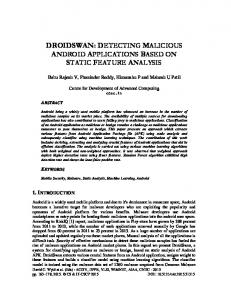
In this section, the proposed method is outlined. The malware and benign samples in PE format are unpacked using the signature-based unpackers like GUN Packer (http://www. woodmann.com), VM Unpacker (http://www.leechermods.com) and dynamic unpacker, i.e., Ether Unpack (http://ether.gtisc.gatech.edu). Thorough unpacking of samples is an important phase in malware analysis otherwise feature selection phase would be effected. Later, features in the form of mnemonic n-grams, and principal instruction opcodes are extracted from the executable dumps obtained from the unpackers. Redundant features are extracted with methods such as CDF, scatter criteria (SC) or PCA. The primary role of all feature ranking methods is to reduce the dimensionality of the feature space. Classifiers are trained using malware (packed and obfuscated), benign samples, and tested with two different test sets. Test set1 consists of obfuscated malware samples and test set2 include packed malware samples. The samples are classified using classification algorithms like IBK, J48, AdaBoost1, random forest and SMO. Figure 1 depicts different phases involved in classifying samples (malware/benign).
210
P. Vinod et al.
Figure 1
5
Proposed model for classifying malware and benign samples
Unpacking executable
Executable packing (Yan et al., 2008) is the process of compressing/encrypting an executable file. A stub is added for decompressing/decrypting the executable. Reverse-engineering of samples tend to be difficult if the executable is packed. According to authors in Lyda and Hamrock (2007), over 80% of malware are packed or re-packed versions of the same base virus. In Perdisci et al. (2008) the authors observed the presence of packed benign samples to be very low up to 1%. However, unpacking a executable is computationally expensive. If the unpacked malware is analysed for detection, then the malware detector might scan the packer code instead of malicious executable code. Malware unpacking process can be explained briefly by following two steps: •
Reverse engineering the unpacker algorithm, then re-implement the unpacker algorithm in a scripting language. Executing this script on the packed file with OllyDbg (http://www.ollydbg.de) or IDAPro (http://www.datarescue.com/idabase).
•
Run time unpacking by tracking a break point before the execution is transferred to the malicious code. This form of suspicious code analysis requires manual intervention.
Unpacking could also be performed using the generic unpacker like VMPacker or GUNPacker. The basic problems with these signature-based packers are: a
signature of packers need to be updated periodically
b
difficulty in the detection of multiple layer packed executables.
For malware employing anti-debugging and anti-unpacking feature, identification of packed layer is a tedious work Hence, alternate way of software unpacking can be performed by using Ether Unpack (http://ether.gtisc.gatech.edu/). The main problem using Ether is that it requires dedicated operating system and hardware. Initially, the sample to be unpacked is executed in the guest operating system (Windows XP SP2) and Ether attempt to locate all memory writes that are performed while the process executes. Whenever a memory write operation is performed the process dump is stored under the
Detecting malicious files using non-signature-based methods
211
images directory. Ether considers each memory write operation as the candidate original entry point (OEP). Figure 2 depict the process of unpacking executables (malware/ benign) using signature-based packers and Ether Unpack. Figure 2
6
PE unpacking procedure
Malware features
Feature is synonymous with input variables or attributes. The key idea is to select relevant (discriminant) attributes or patterns existing with higher frequency to classify a sample as malware or benign. We have extracted mnemonic n-grams and instruction opcodes. Following are the different ways by which the features are extracted: •
Mnemonic n-gram: The author in Bilar (2007) proposed a statistical approach where the opcode frequency distribution of malware and benign programs were compared. It was reported that the opcode distribution for malicious and benign program differed significantly. Motivated by their work, we have used mnemonics as features for classification as they capture difference in malware and benign file sequence. As mnemonics represent the operations to be performed, they can not always be completely replaced by some opcode sequence as the number of equivalent operations are limited. Thus, the structure of program cannot undergo substantial change (Walenstein et al., 2007).
212
P. Vinod et al. Mnemonic n-grams of malware and benign samples are extracted as features. Basically, n-grams are overlapping sub-strings of length n collected in a sliding window fashion. n-grams have found importance in text categorisation and identifying the types of file (Li et al., 2005). We have extracted mnemonic n-gram from assembly code of the malware and benign program. For the following code sample, the bi-grams, tri-grams, quad-grams and larger n-grams are listed. push ebx push esi push [esp+Length] mov ebx, 0C0000001h push [esp+4+Base] push 0 call ds:MmCreateMdl mov esi, eax test esi, esi 2-gram: pushpush pushpush pushmov movpush · · · 3-gram: pushpushpush pushpushmov pushmovpush · · · 4-gram: pushpushpushmov pushpushmovpush pushcallmovtest · · · 5-gram: pushpushpushmovpush pushpushmovpushpush · · ·
•
Instruction opcode extraction: In this method, the opcodes corresponding to instructions are extracted by targeting the executable sections of a PE sample. We have considered onlyWin32 PE format, as majority of the malware compromise Windows operating systems. Following are the different phases of our proposed scheme. a extract sections of PE file and identify executable sections b extract different opcodes of length 1 byte, 2 byte, 3 byte, etc., from raw data present in the sections.
6.1 Extraction of code section The PE file header begins with a MS-DOS header, i.e., IMAGE_DOS_HEADER defined in winnt.h. Two important fields are e_magic and e_lfanew. The e_magic field contain a value 0x5A4D representing DOS signature. The e_lfanew field contain the file offset for PE header. First, the validity of PE sample is examined. All valid PE has e_lfanew = ‘PE\0\0’, otherwise the sample is flagged as invalid PE executable. Figure 3 depict the steps used for validating an executable as a PE file.
Detecting malicious files using non-signature-based methods Figure 3
213
Feature selection: detecting a valid PE
Immediately following the PE signature is IMAGE_NT_HEADER a structure of PE Header. FILE HEADER is one of the member of PE header, designating the physical layout, characteristics, number of sections. Characteristics field indicate the attributes of the file, i.e., whether it is an executable or DLL. If the file is an executable image, the flag IMAGE_FILE_EXECUTABLE_IMAGE contain a value 0x0002. The field NumberOfSections convey total sections present in the executable and gives the size of section table following the PE header. Optional header is skipped as it contains no useful information for our purpose. The sectional header follows the optional header. The Characteristics field of sectional header indicate attributes of sections (like code, data, readable or writeable). If the value of the flag is 0x00000020, it designate that the section contain code. Using PointerToRawData field, the first page of section is located and the complete section is read until SizeOfRawData which furnish the size of section. In this way, the complete raw stream corresponding to code section is extracted. Figure 4 depicts the extraction of raw streams from code section of a PE sample.
214 Figure 4
P. Vinod et al. Feature selection: extraction of bytes from executable sections
6.2 Extraction of opcode The raw information obtained from the code section is used for extracting the opcodes. This step makes binary analysis simple by considering the sequence of raw bytes and transforming them in the form of either opcodes or mnemonics. In order to disassemble the raw sequence into a readable form, ample understanding of x86 instruction format is necessary. A typical x86 instruction contains instruction prefix, opcode, ModR/M, SIB, mode of addressing, etc., (http://www.intel.com/products/processor/ manuals/index.html).
Detecting malicious files using non-signature-based methods
215
Following are the phases involved in extracting the opcodes from the raw stream gathered from code section. •
record all prefixes (values 66 and 67) from the raw stream and eliminate them
•
read the opcode subsequently consult the Opcode Decision table to determine the appropriate ModR/M
•
extract ModR/M byte that defines addressing modes.
Consider a executable file Sample.exe the Hex dump can be visualised in Figure 5. Here 66 is Instruction Prefix, 81, 38 are opcode (1 byte) and ModR/M bytes. Memory and immediate addresses represented by 4D and 5A are also not considered. Therefore, the instruction opcode finally extracted is 8,138. Figure 5
7
An example of instruction HEX dump
Feature processing phase
We have identified features like mnemonic n-grams and instruction opcodes for statistical analysis of malware samples. These features can be used as an elementary means for classification of suspicious samples. It is possible that all attributes extracted from a sample might not convey useful information. Hence, some attributes are required to be eliminated to reduce the excess processing time spent in the training and testing phase. We have used following feature reduction methods: •
CDF
•
SC
•
PCA.
7.1 Class-wise document frequency CDF is a method of filtering out superfluous information to create productive features space (Yang and Jan, 1997). Each program (malware or benign) is transformed into a vector of n-gram for n = 1, 2, 3, 4, 5 and the frequency of the respective n-gram is determined. n-grams common to both malware and benign dataset are identified and their frequencies are computed. Mnemonic n-grams with substantial difference in values in both the target classes are selected for preparing the feature vectors. Training models for each n-gram are created using various classifiers. The n-gram model best suitable for classification is determined based on low FP values. Definition: If the classes of assembly programs are represented by C, the CDF F(η) for n-gram η is given by following equation.
216
P. Vinod et al. F ( η) =
∑ ∑
pi (v, C ) log
C∈{M , B}
i
pi (v, C ) pi (v) pi (C )
where C is either malware (m) or benign (b) and v is a binary value 1(0) signifies that n-gram η is present (absent) in a program. pi(v, C) is the proportion of the program (malware or benign) in which n-gram is present. pi(v) is the proportion of programs having η as n-gram. p(C) is the proportion of program belonging to class {M, B}.
7.2 Scatter criteria The scatter criterion select a feature based on the ratio of the mixture scatter and within class scatter. The mixture scatter is the sum of within and between-class scatter. High value of this ratio indicate prominence and relevance of a feature for prediction. The within-class scatter for a feature f is computed as: |C |
S w, f =
∑p S k
kf
k =0
where C is the set of classes, |C| is the total number of classes, Skf is the variance of feature in class Ck, and pk is the prior probability for a class Ck. The variance Skf can be computed as follows: Skf =
1 N
N
∑ (ζ
i k, f
− ζ k, f
i =1
)
2
where ζ ki , f denotes the ith instance of feature f in class Ck. Between class scatter Sb,f is computed by determining the variance of class centres with respect to a global centre and computed as: Sb , f =
1 |C|
|C |
∑ p (ζ k
k =1
k, f
−ζf
)
2
ζk,f is the mean of feature f in class Ck and ζf is the overall mean of feature f. Mixture Scatter Sm,f is given by: S m , f = S w, f + Sb , f
Scatter criterion for feature f is thus Hf =
Sm, f S w, f
A large value of Hf, for a feature f, is an indicator of the feature being more discriminant for classification.
Detecting malicious files using non-signature-based methods
217
7.3 Principal component analysis PCA is used for attribute selection. Using PCA, features with similar information are grouped together. The organisation of attribute(s) are performed by determining the correlation between the features. If the correlation between any two attributes is high, it indicates that the attributes carry near similar information. Therefore, instead of retaining two attributes, only a single attribute can be used to develop classification model. Assessment of distinct groups can be performed by determining the eigenvalues from the correlation matrix. We estimate k principal components by finding m eigenvectors having largest eigenvalues of the covariance matrix of the dataset.
8
Proposed method for malware analysis using mnemonics n-grams
In the present section, we outline mnemonic n-grams based method. Figure 6 depicts the proposed methodology adopted for detecting suspicious samples. Figure 6
Proposed model for malware an alysis using mnemonic n-grams
•
Malware (packed, obfuscated) and benign executables in PE format are collected and disassembled using the IDA-Pro disassembler (http://www.datarescue.com/idabase).
•
The assembly program obtained from the disassembler is parsed to extract the mnemonics.
218
P. Vinod et al.
•
Mnemonic n-gram (for n = 1, 2, 3, 4, 5) for each sample is generated.
•
Two sets of prominent features are obtained using feature ranking methods such as CDF and scatter criterion. For each set of features, a vector space model is created considering malware and benign instances.
•
n-gram models for n = 1, 2, 3, 4, 5 are prepared employing classifiers like IBK, J48, AdaBoost1, random forest and SMO.
•
To validate the effectiveness of the proposed work, two different test sets is used, containing: a obfuscated b packed malware samples. The outcome of the test is evaluated using the evaluation metrics like true positive rate (TPR), true negative rate (TNR), FPR and false negative rate (FNR).
8.1 Experimental setup A collection of 2,375 malicious samples (http://vx.netlux.org) and 1,437 benign samples (including executables from system32 folder of fresh installation of Windows XP operating system, games, network monitoring utilities, media players and programs, etc.) are divided into two groups to create train and test dataset. The training set consists of 1,135 malicious and 1,067 benign samples. For testing, malware samples are further divided into two groups: •
Test set1 (719 executables) consisting of obfuscated samples.
•
Test set2 (501 executables) consisting of packed malware samples. Malware packed using UPX (http://sourceforge.net/projects/upx/)are primarily used in test set2 as majority of submitted malware are packed using this packer (https://www.virustotal.com).
The benign test set consists of 368 executables. The experiments were performed on an Intel Pentium Core 2 Duo 2.19 GHz processor with 2GB RAM with Microsoft Windows XP SP2 installed on these machines. Following features were obtained for each value of n = 1, 2, 3, 4, 5. •
prominent features obtained using CDF
•
prominent features obtained using scatter criterion
•
mnemonic n-grams present in benign samples but absent in malware samples (discriminant benign features)
•
mnemonic n-grams present in malware samples but absent in benign samples (discriminant malware features).
8.2 Evaluation metrics Results of experiments are evaluated using evaluation metrics like TPR, TNR, FPR, FNR (Tan et al., 2005). These metrics are computed using true positives (TP), true negative
Detecting malicious files using non-signature-based methods
219
(TN), FP and false negative (FN). TP indicates the number of correctly classified malware samples, TN is the number of correctly classified benign instances, FP is the number of benign samples incorrectly classified as malware and FN is the malicious samples classified as benign. The performance of a classifier can be measured by primarily recording the TPR and TNR which are also known as sensitivity and specificity respectively. •
TPR: Corresponds to the proportion of malware samples correctly predicted by the classification model, defined as follows. TPR = TP (TP + FN )
•
FNR: Proportion of malware samples misclassified as benign. FNR = FN ( FN + TP)
•
TNR: Corresponds to the proportion of correctly identified benign samples. TNR = TN (TN + FP )
•
FPR: Proportion of benign samples wrongly predicted as malware by the classification model and is defined as follows. FPR = FP ( FP + TN )
For an effective malware detector, high value of TPR, TNR along with low FPR and FNR is expected. This would ascertain that the scanner is capable of identifying samples with high accuracy.
8.3 CDF features In order to reduce the feature space by removing unwanted attributes with high correlation, we have used CDF. Performing extensive experimentation we reduced the total feature space to 124 prominent features. Table 1 shows top ten attributes/features extracted using CDF. The experimental results demonstrate that the best classification is obtained with the 4-gram model. Table 1
Prominent CDF features
1-gram
2-gram
3-gram
4-gram
5-gram
add
addadd
addaddadd
addaddmovmov
callmovmovmovlea
and
addand
addaddcmp
addcmpjnzmov
callmovmovmovmov
call
addcall
addaddmov
addleamovmov
cmpjzcmpjnzmov
cld
addcmp
addcallmov
addmovaddmov
cmpjzcmpjzcmp
cmp
adddec
addcmpja
addmovcallmov
jmpmovjmpmovjmp
dec
addinc
addcmpjb
addmovcmpjnz
jmpmovmovmovmov
imul
addjmp
addcmpjbe
addmovleamov
jmppushpushpushpush
inc
addlea
addcmpjnb
addmovleapush
jzcmpjzcmpjnz
ja
addmov
addcmpjnz
addmovmovadd
jzpushpushpushpush
jb
addpop
addcmpjz
addmovmovjmp
movcmpjzcmpjnz
220
P. Vinod et al.
Table 2 depicts the values of TPR, TNR, FNR, FPR averaged over different classifiers. Experimental results indicate that random forest performs better in all cases but the performance of other classifiers is very close to random forest. For 4-gram model, we can observe that the TPR is 0.94, TNR is 0.98 with low FNR (0.06) and FPR (0.02) values. We noticed that, 4-gram model is better compared to 3-gram and 5-gram models. On analysis of the feature vector table for 3-gram and 5-gram we found that the features appeared in fewer files (also known as rare features). Thus, the representative values corresponding to many features in the feature vector table were found to be zero. In an n-gram model n represents temporal snapshot presented to the classifier. As n increases the numbers of feature points are reduced even though more information is available to the classifier. Thus, if n is too large a sequence of instruction may not be relevant. Table 2
Mean evaluation metrics for (test set1 and benign samples)
n-grams
TPR
FNR
TNR
FPR
1-gram 2-gram 3-gram 4-gram 5-gram
0.91 0.91 0.93 0.94 0.95
0.09 0.09 0.07 0.06 0.05
0.90 0.93 0.85 0.98 0.73
0.03 0.04 0.20 0.02 0.30
Table 3 presents the evaluation results for test set2 and benign samples. Similar observations are noticed for 4-gram model with better TPR, TNR and low FPR, FNR values. Table 3
Mean evaluation metrics (test set2 and benign samples)
n-grams
TPR
FNR
TNR
FPR
1-gram 2-gram 3-gram 4-gram 5-gram
0.411 0.692 0.923 0.949 0.958
0.589 0.308 0.077 0.051 0.042
0.90 0.93 0.85 0.98 0.73
0.03 0.04 0.20 0.02 0.30
We see from Table 4 that IBK and RF outperform other classifiers in terms of high values of TPR, TNR and small values of FNR, FPR. This indicates that samples are classified perfectly with minimum false prediction. TPR, TNR, FPR, FNR values obtained from different classifiers are shown in Table 5. We infer that RF and SMO perform better as compared to other classifiers. From Tables 4 and 5, it can be inferred that RF result in better detection rate for classifying malware (obfuscated, packed) and benign samples in comparison to SMO as TNR value obtained with SMO is less with respect to RF (refer Table 4). Table 4 Metrics TPR TNR FPR FNR
Mean evaluation metric values for classifiers (test set1) IBK
J48
AdaBoost1
RF
SMO
0.9446 0.8944 0.1056 0.1148
0.8964 0.9442 0.0552 0.1036
0.9114 0.9484 0.0516 0.0886
0.9272 0.8956 0.1044 0.0728
0.959 0.6938 0.3056 0.041
Detecting malicious files using non-signature-based methods Table 5 Metrics
221
Mean evaluation metric values for classifiers (test set2) IBK
J48
AdaBoost1
RF
SMO
TPR
0.884
0.962
0.95
0.966
0.98
TNR
0.925
0.99
0.992
0.984
0.99
FPR
0.075
0.01
0.008
0.016
0.01
FNR
0.116
0.038
0.05
0.034
0.02
From the tabulated results, it can be visualised that as the value of n in an n-gram model increases, TPR increases but same is not true for TNR. In our opinion, it may be that benign samples, being more diverse cannot be modelled by the classifiers.
8.4 Features extracted using scatter criterion Scatter criterion is used for extracting discriminant features amongst malware and benign samples. The test is performed on obfuscated malware (unpacked, packed) and benign samples. Table 6 depicts prominent mnemonic n-grams obtained using the scatter criterion. The attributes having higher value of Hf, i.e., scatter criterion (refer Section 7.2) is found promising for the classification of executables. Table 6 1-gram add jbe cmp or test pop jnb jnz jz sub
Prominent mnemonic n-gram obtained using scatter criterion 2-gram
3-gram
4-gram
5-gram
jnzjmp submov calljz sublea movmov movjz leacmp movjnz shlmov cmpjg
pushmovor movaddpop xormovlea movsublea submovlea movmovrep xorpushmov leacmpjz jzmovinc movxorlea
cmpjzmovlea cmpjnbmovmov movmovjmpcmp movjmpmovcmp pushmovsubmov movmovmovadd movmovmovpop movcmpjzcmp movmovmovcmp submovmovmov
movmovmovmovcmp cmpjzcmpjnzmov movmovmovpushmov movmovmovmovmov movmovcmpjzcmp movmovmovmovjmp jzcmpjzcmpjnz movmovmovjmpmov movmovpushmovmov movcmpjzcmpjnz
Table 7 depicts the average values of TPR, TNR, FPR, FNR obtained with various classifiers. We can observe that 4-gram attributes are relevant for better classification of obfuscated/unpacked malware and benign samples. This can be validated as higher values of TPR, TNR and low values of FPR, FNR are obtained with the 4-gram models with respect to other n-gram models. Table 7
Mean evaluation metric values for classifiers (test set1)
n-gram
TPR
FNR
TNR
FPR
1-gram
0.905
0.095
0.897
0.103
2-gram
0.924
0.076
0.899
0.101
3-gram
0.920
0.080
0.837
0.163
4-gram
0.942
0.058
0.800
0.200
5-gram
0.921
0.079
0.724
0.276
222
P. Vinod et al.
To estimate the behaviour of different n-gram models, we tested the models using test set2 and benign samples. Values of TPR, FNR, TNR, FPR were recorded for different n-grams and classifiers (refer Table 8). We can visualise that 4-gram model proves to be better in terms of higher values of TPR = 0.967, TNR = 0.80 and smaller values of FNR, FPR (0.033, 0.21). Table 8
Mean evaluation metric values for classifiers (test set2)
n-gram
TPR
FNR
TNR
FPR
1-gram
0.304
0.696
0.897
0.103
2-gram
0.465
0.535
0.899
0.101
3-gram
0.741
0.259
0.837
0.163
4-gram
0.967
0.033
0.800
0.200
5-gram
0.958
0.042
0.724
0.276
Table 9 displays classification accuracy obtained for 4-gram model using different classifiers like IBK, J48, AdaBoost1, RF and SMO. If we closely examine the values of evaluation metrics, for test set1 and test set2, we can argue that the performance of IBK and RF is better that SMO, as the TNR and FPR values for SMO are less compared to the classifiers IBK and RF. Table 9 Classifiers
Performance of classifiers for 4-gram features Test set1
Test set2
TPR
FNR
TNR
FPR
TPR
FNR
TNR
FPR
IBK
0.947
0.053
0.862
0.138
0.968
0.032
0.862
0.138
J48
0.933
0.067
0.831
0.169
0.962
0.038
0.831
0.169
AdaBoost1
0.924
0.076
0.837
0.163
0.950
0.050
0.837
0.163
RF
0.944
0.056
0.837
0.163
0.960
0.040
0.837
0.163
SMO
0.960
0.040
0.613
0.387
0.976
0.024
0.613
0.387
8.5 Discriminant attributes of benign and malware samples The classifiers are trained with feature vectors for different n-grams consisting of 2202 executable (benign and malware). As with all previous experiments, the test set was separated into two: •
first set consisting of 719 malware (obfuscated and unpacked), 368 benign samples
•
second set consisting of 501 malware (obfuscated and packed) and 368 benign samples.
Two different categories of features are extracted: a
discriminant features of benign samples
b
discriminant features of malware samples.
Tables 10 and 11 depict discriminant features present in benign and malware samples for different n-grams (n = 1, 2, 3, 4, 5).
Detecting malicious files using non-signature-based methods Table 10 1-gram int
223
Discriminant n-grams in benign samples 2-gram
3-gram
4-gram
5-gram
intint
intintint
intintintint
intintintintint
fld
calljnz
callmovjz
movjzmovmov
callpushmovpushpush
fstp
notmov
callmovjnz
movmovmovjz
movmovmovmovjz
fild
movnot
movjzcmp
callmovjzmov
movjzmovmovmov
–
intpush
calljzmov
movjnzmovmov
movmovjzmovmov
–
jzjz
calljnzmov
movmovjnzmov
movmovmovjzmov
–
movjle
movmovjnz
movmovmovjnz
callmovcmpjzcmp
–
jmpint
movjnzpush
movjzcmpjnz
movcallpushmovpush
–
leajz
movjzlea
calljzmovmov
cmpjnzmovmovcmp
–
notjmp
movcalljnz
movjzcmpjz
pushmovsubmovmov
Table 11
Discriminant n-grams in malware samples
1-gram
2-gram
3-gram
4-gram
5-gram
add
addmov
movaddmov
movaddmovmov
movmovaddmovmov
pop
movadd
addmovmov
movmovaddmov
pushpushpushcallpop
or
addpush
movmovadd
addmovmovmov
movaddmovmovmov
test
poppop
pushcallpop
movmovmovadd
addmovmovmovmov
xchg
popmov
movaddpush
pushpushcallpop
pushpushcallpoppop
cld
movpop
poppoppop
pushpushcalltest
movmovmovaddmov
stosb
callpop
addpushpush
pushcalltestjz
pushpushcalltestjz
leave
addcmp
addmovadd
popretnpushmov
movmovmovmovadd
repne
popretn
pushmovadd
movaddpushpush
pushpushcalltestjnz
loop
testjz
pushcalltest
movaddmovadd
movpopretnpushmov
Table 12 shows the TPR, FNR, TNR, FPR values for obfuscated malware (unpacked, packed) and benign samples. The n-gram model is prepared using features present in benign and absent in malware samples. The training model is developed using IBK, J48, AdaBoost1, RF, SMO classifiers. Examining Table 12, we can argue that 4-gram model is suitable for better classification of samples. In this table, we present the average classification results obtained with different classifiers for both test sets (i.e., set1 and set2). Table 12 n-gram
Evaluation metric values for discriminant benign features Test set1
Test set2
TPR
FNR
TNR
FPR
TPR
FNR
TNR
FPR
1-gram
0.874
0.126
0.860
0.140
0.811
0.189
0.860
0.140
2-gram
0.914
0.086
0.881
0.119
0.737
0.263
0.881
0.119
3-gram
0.945
0.055
0.731
0.269
0.965
0.035
0.731
0.269
4-gram
0.950
0.050
0.704
0.296
0.969
0.031
0.704
0.296
5-gram
0.949
0.051
0.634
0.366
0.969
0.031
0.634
0.366
224
P. Vinod et al.
The classification accuracy for the features present in malware samples and absent in benign samples was found to be very less. This can be observed from the TPR, FNR, TNR, FPR values in Table 13. Also, the results obtained from test set2 were appreciable. When the feature vector was closely monitored, we noticed that very few mnemonic patterns of test samples (test set2) were found in the entire dataset. Table 13
Evaluation metric for discriminant malware features
n-gram
TPR
FNR
TNR
FPR
1-gram
0.787
0.213
0.986
0.014
2-gram
0.771
0.229
0.997
0.003
3-gram
0.773
0.227
1.000
0.000
4-gram
0.823
0.177
0.982
0.018
5-gram
0.795
0.205
1.000
0.000
Table 14 shows information for different n-gram models like a
number of features present in malware but absent in benign samples (M-B)
b
difference of features present in M-B and packed samples of malware shown as Diff(M-B, packed)
c
common features present in M-B and packed malware samples represented as Common(M-B, packed).
The classification accuracy obtained is very less with respect to the accuracies of other feature category discussed in previous experiment, as the discriminant malware attributes were rarely present in packed samples. Table 14
Common and discriminant features of M-B and test set2 samples for n-grams
n-gram
M-B
Diff(M-B, packed)
Common(M-B, packed)
1-gram
16
13
3
2-gram
107
98
9
3-gram
224
210
14
4-gram
234
227
7
5-gram
151
148
3
9
Analysis of results
In the proposed method, we have outlined statistical approach based on mnemonic n-grams for analysis and detection of malware. On the basis of results tabulated in Tables 2 to 14 the outcome of the experiments can be summarised as below: a
The proposed method can be used for assisting the scanners for classifying the samples at a preliminary stage.
Detecting malicious files using non-signature-based methods
225
b
The detection accuracy of the proposed method is just reasonable and comparable to previously published results. This is indicated by a high TPR and low FNR.
c
The proposed detection method identifies both packed/obfuscated malware samples.
d
The proposed prototype also performs in identifying unseen benign samples (TNR = 0.98, FPR = 0.02).
e
The classification model for 4-gram proves to be better compared to all other models. The primary reason for misclassification with other n-gram models is the presence of features with null value (absence in many samples) representation of the feature vector table.
f
The classification accuracies obtained using the feature reduction methods like CDF and SC are comparable.
g
The behaviour of classifiers like IBK and RF are better for classifying malware (packed and obfuscated) and benign samples. The better result is obtained in case of random forest as it is an ensemble-based classifier which aggregates the result of multiple classifier to predict the class.
In conclusion, we can argue that the proposed method using mnemonic n-gram feature can be used to identify packed, unpacked, and obfuscated malware samples. The experimental results depict that as n increases TPR also increases. This is due to the fact that the code distortion or variations are not much pronounced in case of malware variants used in our dataset (http://vx.netlux.org). Primarily, the malware code is embedded with a small engine that mutates the base code to generate variants. Size of mutation engine cannot be too big to avoid detection and also there are limited number of opcode replacements that are possible (Chouchane et al., 2006). Thus, it can be inferred that code variability cannot be too significant in malware samples. But, in case of the benign instances the diversity in the code is more as each benign sample have different behaviour. Thus, the value of TNR does not significantly increase for different values of n. Therefore, it can be argued that unlike malware samples an abstract model for benign instances cannot be formulated. In comparison to previous work, we consider obfuscated and packed samples for model construction and prediction. Hence, the feature selection phase would be effected if we consider packed samples. The primary reason is that, the disassembler would output assembly code of packer or outer layer executable. Also, the feature vector length in our experiment is comparatively less compared to prior work reported in the literature. This is significant in view of processing time requirement.
10 Proposed method for malware analysis using principal instruction opcodes In this proposed scheme, we make use of Principal Instruction opcodes of samples (malware or benign) as features. The term principal in this context refers to those prominent instruction opcodes obtained using PCA or scatter criterion (as part of feature reduction). Let us consider two instructions:
226
P. Vinod et al. MOV Reg, M
MOV M, Reg
The 2-gram mnemonic pattern for the above instructions is movmov. The n-gram representation does not give complete information of the instructions. As the Hex code representation of both the instructions are different. In order to have a better understanding of the instruction as compared to mnemonic n-gram, we extracted the Hex code representation (refer Section 6.2) of instruction which include the type of operations as well as the addressing mode. We refer to this representation of the instruction as instruction opcode. Following steps were performed for extracting principal instruction opcode using PCA: 1
Extract instruction opcodes occurring with high frequency in samples (malware/benign). Also, these opcode should indicate variance in target classes. All samples are represented in the form of a column vector of size MX1, where M is the total feature space. Therefore, N training samples are arranged in the form of MXN vector.
2
Average vector for training set is computed and each file is normalised (mean subtracted value is computed). Later, the eigenvalues and eigenvectors are determined. Subsequently, the eigenvectors are arranged with respect to decreasing eigenvalues.
3
Select relevant instruction opcodes by fixing a lower threshold value (in our case we assumed 0.01). This conforms to prominent features to be used for classification.
4
Vector space models are created for malware and benign instances which are used for model preparation and later in prediction phase.
Consider an example of feature extraction using PCA. Table 15 depicts instruction opcodes in the first row and their frequencies in each sample in the subsequent rows. Fi represents malware or benign samples for instance i. Using PCA, each program represents a point in the n-dimensional opcode space, with instruction opcodes representing one of the axes. The eigenvalues are computed and subsequently eigenvectors are determined for largest eigenvalues. Table 15
Instruction opcode frequencies in each file Fi
Samples\opcodes
0x04
0x0F84
0x0F85
F1
20
04
100
F2
10
15
90
F3
82
327
161
F4
1
11
8
Table 16 exhibits an example of eigenvectors corresponding to the eigenvalues. An eigenvector is indicative of relative weight of each opcode. Eigenvectors with the highest eigenvalue act as the principal component. For constructing features, absolute value of eigenvalues are considered. If we deal with the union of all instruction opcodes extracted from eigenvectors, the relevant features of malware and benign samples are obtained.
Detecting malicious files using non-signature-based methods Table 16
227
Eigenvectors corresponding to eigenvalues
Opcodes\eigenvalues
EV1
EV2
EV3
0x04
0.601
–0.189
0.776
0x0F84
0.578
–0.568
–0.586
0x0F85
0.552
0.801
–0.232
•
Input:
•
a
EV = {E1 , E2
b
λ = {λ1 , λ2
c
N and τ
d
flag = FALSE.
Em } λm }
▷EV: set of eigen vector. ▷λ: set of eigen values. ▷Total feature space and threshold.
Output: a
•
O Plist = {op1 , op2 , …… , opk } .
▷Prominent opcode(s).
Steps:
Algorithm 1 1 2 3 4 5 6 7 8 9 10 11
for i = 1 to N do Sort(EVi, λi) end for OPlist = NULL for i = 0 to k do newOpcodei = extractInstOpcode(EVi, τ) flag = findInstOpcode(newOpcodei, OPlist) if flag == False then OPist = OPlist ∪ newOpcodei end if end for
Algorithm 1 present the method adopted for selecting prominent instruction opcode using PCA. Once the features are determined, a vector space model is created using the frequencies of the opcodes for training samples in the dataset. Each row of the dataset (instance of malware or benign) is labelled as M or B, where M represents malware and B stands for benign.
10.1 Experimental setup Experiments were performed on dataset consisting of 4,546 Win32 PE executables. This dataset contains 1,129 viruses downloaded from VX Heavens (http://vx.netlux.org) a repository of malware. We obtained 1,085 benign programs from System32 folder of fresh installation of Windows XP operating system, some from Cygwin (http://www.cygwin.com/) utility, games, internet browsers, media players and other sources. The experiments were carried out using WEKA (http://www.cs.waikato.ac.nz)
228
P. Vinod et al.
for training and later for testing phase. The training set consisted of 2,214 samples (malware = 1,129 and benign = 1,085). Two test sets were created: •
test set1 consisting of 439 obfuscated malware and 443 benign samples
•
test set2 consisting of 596 packed malware and 845 benign samples.
The test set is kept separate and none of these samples are included for feature extraction. The experiments were performed using SMO, IBK, AdaBoost1 (with J-48 as base classifier), J-48 and random forest algorithms implemented in WEKA. The results are evaluated using the evaluation metrics defined in Section 8.2. For each experiment, categories of features are extracted for preparing feature vectors which are given below: •
instruction opcodes which are predominant in malware but occur with less frequency in benign samples (refer Table 17)
•
instruction opcodes which are predominant in benign but have less frequency in malware samples (refer Table 17)
•
discriminant malware instruction opcodes (M\B) (refer Table 18)
•
discriminant benign instruction opcodes (B\M) (refer Table 18).
Table 17
Predominant instruction opcodes for malware and benign files
Malware
Benign
0X00FF 0X06 0X0D 0X24 0X25 0X2C 0X2D 0X33C0 0X35 0X3C
0X04 0X0F84 0X1C 0X2D 0X40 0X48 0X50 0X56 0X59 0X68
Table 18
Discriminant instruction opcodes of malware and benign samples
No.
Benign (B-M)
No. files
Malware (M-B)
No. files
1
0X8975
992
0X6F
719
2
0X895D
976
0X6E
701
3
0X8901
962
0X6D
666
4
0X81EC
957
0X54
663
5
0X897D
955
0X60
618
6
0X8908
893
0X4C
578
7
0X83FF
879
0X5C
551
8
0X8B15
874
0X696E
534
9
0X83FA
870
0X8BE5
532
10
0X3B45
864
0XAC
521
Detecting malicious files using non-signature-based methods
10.2
229
Predominant features of malware samples
Features are extracted from 1,129 malware samples using PCA. We obtain features consisting of 91 principal instruction opcodes. Once the features are extracted, we construct feature vector for 2,214 executable files (malware and benign), where each instance is labelled as {M, B}. The best classification was obtained for random forest with: a
test set1 (TPR = 0.961, FNR = 0.041, TNR = 0.898, FPR = 0.101)
b
test set2 (TPR = 0.956, FNR = 0.043, TNR = 0.823, FPR = 0.176).
Table 19 depicts the values of evaluation metrics obtained with different classifiers for Test set1. Table 20 exhibits the sensitivity and specificity values obtained with different classifiers for test set2. Table 19
Evaluation metrics for 91 malware features (test set1)
Classifier
TPR
FNR
TNR
FPR
SMO IBK AdaBoost1 J48 RF
0.881 0.881 0.917 0.924 0.961
0.12 0.12 0.091 0.079 0.041
0.37 0.896 0.925 0.902 0.898
0.629 0.103 0.074 0.088 0.101
Table 20
Evaluation metrics for 91 malware features (test set2)
Classifier
TPR
FNR
TNR
FPR
SMO IBK AdaBoost1 J48 RF
0.981 0.949 0.958 0.827 0.956
0.0184 0.05 0.041 0.172 0.043
0.436 0.814 0.854 0.809 0.823
0.563 0.185 0.145 0.19 0.176
10.3 Predominant features of benign executables Features were extracted from 1,085 benign programs using PCA. We trained classifiers with labelled feature vectors using 2,214 executables. Using PCA, feature vector length of 35 principal instruction opcodes are extracted. Similar to the previous experiment, the best classification accuracy is obtained for random forest with a
test set1 (TPR = 0.961, FNR = 0.038, TNR = 0.898, FPR = 0.101) refer Table 21
b
test set2 (TPR = 0.958, FNR = 0.041, TNR = 0.838, FPR = 0.161) (refer Table 22).
Table 21
Evaluation metric for 35 predominant benign features (test set1)
Classifier
TPR
FNR
TNR
FPR
SMO IBK AdaBoost1 J48 RF
0.881 0.881 0.917 0.922 0.961
0.118 0.118 0.082 0.077 0.038
0.37 0.896 0.925 0.902 0.898
0.629 0.103 0.074 0.088 0.101
230
P. Vinod et al.
Table 22
Evaluation metric for 35 predominant benign features (test set2)
Classifier
TPR
FNR
TNR
FPR
SMO
0.979
0.02
0.313
0.686
IBK
0.926
0.073
0.802
0.197
AdaBoost1
0.949
0.050
0.823
0.176
J48
0.939
0.06
0.843
0.156
RF
0.958
0.041
0.838
0.161
10.4 Discriminant instruction opcodes (benign) Using PCA, we choose instruction opcodes (feature length of 124 opcodes) present only in benign programs and absent in Malware. Table 18 depict discriminant principal instruction opcodes of benign samples along with the number of executables in they appear. For both test sets, random forest outperforms other classifiers (refer Tables 23 and 24) considering classification accuracies. We can observe that the TPR, TNR values obtained from random forest classifier is better compared to other classifiers used in this study. Table 23
Evaluation metrics for discriminant benign instruction opcodes (test set1)
Classifier
TPR
FNR
TNR
FPR
SMO
0.949
0.05
0.559
0.44
IBK
0.904
0.095
0.884
0.115
AdaBoost1
0.89
0.109
0.92
0.079
J48
0.9
0.1
0.871
0.128
RF
0.9
0.1
0.912
0.088
Table 24
Evaluation metrics for discriminant benign instruction opcodes (test set2)
Classifier
TPR
FNR
TNR
FPR
SMO
0.974
0.025
0.503
0.496
IBK
0.954
0.045
0.844
0.155
AdaBoost1
0.932
0.067
0.878
0.121
J48
0.914
0.085
0.8
0.199
RF
0.966
0.033
0.86
0.139
10.5
Discriminant instruction opcodes (malware)
The classifiers were trained with labelled feature vectors for 2,214 executables. Using PCA, we selected opcodes (feature length of 18 opcodes) present only in malware and absent in benign programs. Table 25 depicts the classifier accuracies for different evaluation metrics.
Detecting malicious files using non-signature-based methods Table 25
231
Mean evaluation metrics for discriminant instruction opcodes of malware samples Test set1
Classifiers
Test set2
TPR
FNR
TNR
FPR
TPR
FNR
TNR
FPR
SMO
0.109
0.89
0.945
0.054
0.0939
0.906
0.927
0.072
IBK
0.835
0.164
0.884
0.115
0.85
0.149
0.81
0.189
AdaBoost1
0.829
0.17
0.887
0.112
0.892
0.107
0.779
0.22
J-48
0.808
0.191
0.882
0.117
0.887
0.112
0.806
0.193
Random forest
0.842
0.157
0.857
0.142
0.917
0.082
0.797
0.202
10.6 Extraction of principal instruction opcodes using scatter criterion Scatter criterion (refer Section 7.2) is used to scale down the redundant instruction opcodes from benign and malware executables. For the malware dataset (consisting of 1,129 executables), total 193 distinct instruction opcodes were extracted. Using scatter criterion, the feature space (193 unique instruction opcodes) was reduced to 37 opcodes based on the values of Hf. Likewise, for benign samples (576 instruction opcodes), the feature space was further reduced to 57 prominent opcodes. Classifiers were trained using 2,214 executables (malware/benign) and tested using test set1 (439 obfuscated malware, 443 benign samples) and test set2 (596 packed malware, 854 benign samples). The performance was evaluated using the evaluation metrics of Section 8.2. Tables 26 and 27 depict the classifier accuracies for features gathered using Scatter Criterion for both malware and benign samples. Table 26
Mean evaluation metrics for prominent malware features using SC Test set1
Classifiers
TPR
FNR
Test set2 TNR
FPR
TPR
FNR
TNR
FPR
SMO
0.961
0.038
0.239
0.76
0.981
0.018
0.252
0.747
IBK
0.924
0.075
0.891
0.108
0.963
0.036
0.85
0.149
AdaBoost1
0.922
0.077
0.894
0.101
0.956
0.043
0.854
0.145
J-48
0.927
0.072
0.893
0.106
0.953
0.046
0.833
0.166
Random forest
0.938
0.061
0.891
0.108
0.976
0.023
0.84
0.159
TNR
FPR
Table 27
Mean evaluation metrics for prominent benign features using SC
Classifiers
Test set1 TPR
FNR
Test set2 TNR
FPR
TPR
FNR
SMO
0.867
0.132
0.273
0.726
0.978
0.021
0.282
0.717
IBK
0.917
0.082
0.889
0.11
0.953
0.046
0.827
0.172
AdaBoost1
0.908
0.091
0.905
0.094
0.959
0.04
0.867
0.132
J-48
0.89
0.109
0.909
0.09
0.922
0.077
0.855
0.144
Random forest
0.927
0.072
0.911
0.088
0.961
0.038
0.852
0.147
232
P. Vinod et al.
11 Analysis of results In non-signature-based method, we have proposed malware analysis using machine learning methods, which is capable of detecting unseen malware specimens. Prominent instruction opcodes were extracted using PCA and scatter criterion. From our experiments as tabulated above (Tables 19 to 27), we observe that better classification accuracy with low false alarms is obtained. Some important observations made from the experiments are listed below: a
The detection accuracy of the proposed method (using PCA) is reasonable. This can be validated by a high TPR = 0.96 and low FNR = 0.04 for test set1.
b
The proposed detection methods is suitable for identifying both packed/obfuscated malware samples.
c
The proposed prototype also performs better for classifying unseen benign samples.
d
The behaviour of classifiers like AdaBoost1 and random forest is better for classifying malware (packed and obfuscated) and benign samples. The main reason for better classification is because the former is based on bagging and boosting and later uses ensemble method for predicting specimens.
e
Comparing the features obtained using PCA and scatter criterion we observe that better classification accuracies are obtained with features extracted using PCA.
Figures 7 and 8 depict that for both test sets (test set1 and test set2) the predominant features of malware (M) or benign (B) samples results in better detection rate as compared to discriminant features of malware (M\B) or benign (B\M). Figure 7
Sensitivity v/s specificity for test set1 (see online version for colours)
Detecting malicious files using non-signature-based methods Figure 8
233
Sensitivity v/s specificity for test set2 (see online version for colours)
We observe that using the second method improved detection accuracy over the method based on n-gram feature. This experiment also shows improved performance for identifying packed, unpacked and obfuscated malware and benign files. Classification accuracies obtained for predominant features collected for malware/benign samples are superior compared to the discriminant attributes. This may be because most benign program are written in high level languages and translator (compiler) is likely to use a subset of instruction(s) and or addressing modes more frequently. Malware are wholly or partially developed in assembly language. So, the malware program contain instruction(s) or addressing modes not likely to be encountered in benign. Thus, the discriminating subset is likely to be malware author specific as a result these features do not appear predominantly. In all previous work reported in literature, top 300 or more features were selected and accuracies were measured. Using extensive experiments we selected top 35 principal instruction opcodes with the feature extraction method and achieved a better detection rate of 96% for malware and benign samples. Our approach also is suitable for imbalance dataset where the proportion of malware samples are comparatively less than benign executables. Figure 9
Proposed model using ensemble-based feature selection and ensemble-based classifiers for identifying malware and benign executables
234
P. Vinod et al.
In order to increase the accuracy, we feel that an approach which generate aggregated feature list from different features selection method should be adopted (refer Figure 9). If common prominent features are extracted from different feature selection methods, we feel that the feature space would substantially decrease. This might further increase the accuracy as the aggregated feature list would consist all prominent features from different feature selection methods. Also, classification using ensemble-based technique would be appropriate as ensemble method capture strength of individual classifier for the effective classification of executables (malware or benign).
12 Running time In Table 28, we show the time required (feature extraction) for different types of features (n-gram and instruction opcode). The feature extraction process includes unpacking (signature-based packers and Ether Unpack) and disassembling of executables. Executable unpacking is a time consuming process and if the executable is not unpacked it would further affect the feature selection process. The estimated time to disassemble 4,546 executable is observed to be approximately 180 seconds. Extraction of instruction opcode by our proposed disassembler is 60 seconds. As n increases the time required for feature extraction also increases. Table 28
Running times in seconds for different n-gram models
n-gram
Process feature
Total time (disassembling and feature processing)
Per sample time
1-gram 2-gram 3-gram 4-gram 5-gram
28 69 289 891 1,758
208 249 469 1,071 1,938
0.045 0.054 0.103 0.235 0.426
Table 29 shows the time required for classifying executables by different classifiers. Here, we rank the execution time in the scale of 1 to 5 where ‘5’ depict the minimum and ‘1’ shows maximum time for classification. Thus, we have noticed that the random forest classifier has better detection rates but the running time for the classifier is highest compared to all other classifiers. In case of perfect detection system the training model needs to be upgraded as predominant features are likely to change by time, we feel that the running time of the detection system would also gradually change. Table 29 Classifier IBK SMO J-48 AdaBoost1 RF
execution time ranked on a scale of ‘1’ to ‘5’ for classifying executables using different classifier Rank 5 3 4 2 1
Detecting malicious files using non-signature-based methods
235
In order to reduce the malware unpacking time we need to automate the process of reading the samples from a location, load them into Windows XP guest operating system and unpack them using Ether Unpack. This task is still under progress. However, the extraction of features, feature vector table creation and classification in near to real time detection methods. Thus, the present system could be used for off line scanning of malware executables.
13 Experiments on imbalanced dataset In machine learning domain, an imbalanced dataset is a common experience. In this scenario, a class is consist of more number of instances while the other class is represented by fewer instances. Thus, a classifier correctly classifies instances belonging to the class having larger proportion of samples compared to other class (also known as biased classification). In real world, malware files are less compared to benign executables. Hence, we are interested in investigating if malware files can be detected from the available dataset consisting of larger number of benign executables. Experiments are conducted on 2,430 real malware samples (collected from VX Heavens) and 4,050 benign samples (gathered from System32 folder and different utility software’s™). Benign samples are scanned using commercial antivirus products before including them in the dataset used for experiments. Experiments are performed using different proportions of malware samples, henceforth referred to as proportion of malicious executables (PME). In each experiment, the number of malicious samples considered are X% of benign specimens (where X% is 20%, 30%, 40%, 50% and 60%). For example, for X = 20, if the number of benign samples are 4,050, the number of malicious samples considered are 810 (20% of benign samples). For each value of X, evaluation metrics and accuracy (ACC) are computed. Experiments are conducted on a new features derived by us known as principal instruction opcodes (opcode with addressing modes). Features are preprocessed using PCA. Classification algorithms supported withWEKA on default settings is considered. In all experiments, we have observed that Random Forest classifier (RF) outperformed other classifiers. Hence, only the results for RF is reported for different experiments due to lack of space.
13.1 Cross-validation Cross-validation is a method used in data mining for estimating the performance of a given model. In case of k cross-validation, entire dataset is divided into k subsets of approximately similar size. We have used stratified cross-validation method. In this technique, folds are stratified and the same number of samples are used in each set. The original dataset, D, is divided into subsets D = { D1 , D2 , D3 , , Dk } . Classifiers are trained using k – 1 sets and tested with remaining instances. The process is repeated k times and finally the accuracy of the model is determined. Accuracy of a model is estimated by the ratio of total number of correctly classified instances to the total number of instances in the dataset.
236
P. Vinod et al.
In our study, we used stratified ten-fold cross-validation. Kohavi (1995) performed extensive experimentation on a dataset of half a million instances and proved that ten-fold cross-validation performed best for determination of the accuracy of a model.
13.2
Performance on imbalanced dataset
For malware and benign executables, prominent features were extracted using PCA. By prominent, we mean a set of features predominant in one class as compared to others. Prominent instruction opcodes with varying PME were extracted. As with all previous experiments, we observed that better detection rate was obtained with prominent malware or benign features as depicted in Figures 10 and 11. From Figure 11, we can visualise that for PME value of 20%, an accuracy of 96.5% is obtained with a detection rate (TPR) of 85.2% and TNR value of 98.8%. This accuracy is achieved for feature length of 12 and 64 prominent instruction opcodes extracted from malware and benign executables. It was observed that there was a marginal increase in detection rate with increase in PME values without much difference in accuracy. This can be validated for dataset containing larger proportion of malware as compared to benign, where accuracy of 94.5% is obtained. This is comparable with previous work reported in literature. Figure 10
Accuracies determined with random forest for prominent malware features (see online version for colours)
Detecting malicious files using non-signature-based methods Figure 11
237
Accuracies determined with random forest for prominent benign features (see online version for colours)
14 Conclusions and future work Malicious Software (malware) is a major threat to computer systems. Malware detection mechanisms are gaining prominence amongst researchers and have turned out to be a topic of research. The number of malware has increased at an alarming rate due to the fact that malware writers are deploying obfuscation methods. The non-signature-based detection methods are important as the malware writer are producing metamorphic or polymorphic malware. Thus, signature-based methods cannot detect these modern malware. Therefore, it is required that the signature-based techniques need to be complemented with some non-signature mechanisms for effective detection of malicious software’s™. In this paper, we have proposed a non-signature-based detection techniques capable of identifying obfuscated and packed malware samples. The detection mechanism is performed using two different schemes: a
mnemonic n-gram
b
extraction of principal instruction opcodes.
238
P. Vinod et al.
The experiments were performed using two different test sets-one consisting of obfuscated malware and another having packed malware executables. The system was able to detect obfuscated and packed malware variants. The system was able to effectively differentiate malware and benign samples. The experimental results demonstrated that 4-gram model was found to be superior compared to other mnemonic n-gram models. Using our proposed method of extracting mnemonic n-grams, TPR = 0.95 and TNR = 0.98 was obtained for obfuscated and packed samples. The principal instruction opcodes extracted using our proposed resulted in a detection rate with TPR = 0.961 and TNR = 0.90. Better results have been obtained with predominant features of benign sample with feature length of 35. Benign program are written in high level languages and the translator use subset of instructions and or addressing modes. On the other hand malware code might contain instructions/addressing modes not likely in benign samples and the discriminating instructions in a malcode is author specific. Results also suggests that malware samples can be identified from a large population of benign samples. The experimental results of n-gram depict that as n increases TPR also increases but this is not always the case with TNR. This is because the malware samples are generated by obfuscation engine with limited possibility of instruction substitution. Also, the malware code cannot undergo complete change since the functionality of the program needs to be preserved. Thus, malware transforms itself to generate variants preserving base code which cannot completely change. In case of benign samples the code are highly diverse and functionally independent. Thus, in our view benign samples being more diverse cannot be modelled by classifiers. The results obtained using mnemonic n-gram and instruction opcodes with very small feature length are better compared to prior work reported in literature. We also argue that better classification accuracies are achieved using better feature selection algorithms. Thus, for perfect detection system we feel that the selection of effective feature selection methods and inducer algorithms for classifier play a vital role in appropriate classification of the instances. The present detection system can be used as a off line malware scanner as unpacking is time consuming activity. The time for disassembling, feature extraction and classification is near to real time implementation systems. In future, the effect of classification accuracies by using hybrid features (mnemonic n-grams, instruction opcode, APIs and some PE structural information) will be worked upon for observation. In future, we would like to investigate on new information theoretic feature selection and feature extraction methods to extract robust features with fewer length for classification and prediction. We also feel that, the location-based opcode feature may yield some promising results. This feature might reveal important insight for malware detection, as researchers can monitor which block of code is predominantly used. Also, we could investigate if code transposition a paramount obfuscation method used by malware writers as reported in earlier literature.
References Attaluri, S., McGhee, S. and Stamp, M. (2009) ‘Profile hidden Markov models and metamorphic virus detection’, Journal in Computer Virology, Vol. 5, No. 2, pp.151–169. Baysa, D., Low, R.M. and Stamp, M. (2013) ‘Structural entropy and metamorphic malware’, Journal of Computer Virology and Hacking Techniques, Vol. 9, No. 4, pp.1–14, Springer-Verlag.
Detecting malicious files using non-signature-based methods
239
Bilar, D. (2007) ‘Opcodes as predictor for malware’, International Journal Electron Secure Digital Forensic, Vol. 1, No. 2, pp.156–168. Chouchane, M.R. and Lakhotia, A. (2006) ‘Using engine signature to detect metamorphic malware’, Proceedings of the 4th ACM Workshop on Recurring Malcode, WORM’06, pp.73–78, New York, NY, USA. Henchiri, O. and Japkowicz, N. (2006) ‘A feature selection and evaluation scheme for computer virus detection’, Proc. of the Sixth International Conference on Data Mining, ICDM’06, pp.891–895. Karim, M.E., Walenstein, A. and Lakhotia, A. (2005) ‘Malware phylogeny generation using permutations of code’, Journal in Computer Virology, Vol. 1, Nos. 1–2, pp.13–23. Kephart, J.O. and Arnold, B. (1994) ‘A feature selection and evaluation of computer virus signatures’, Proceedings of the 4th Virus Bulletin International Conference, pp.178–184. Kohavi, R. (1995) A Study of Cross-Validation and Bootstrap for Accuracy Estimation and Model Selection, pp.1137–1143, Morgan Kaufmann. Kolter, J.Z. and Maloof, M.A. (2004) ‘Learning to detect malicious executables in the wild’, KDD’04: Proceedings of the Tenth ACM SIGKDD International Conference on Knowledge Discovery and Data Mining, pp.470–478, ACM, New York, NY, USA. Li, W.J., Wang, K., Stolfo, S.J. and Herzog, B. (2005) ‘Fileprints: identifying file types by n-gram analysis’, Proceedings of the Sixth Annual IEEE SMC 4th Virus Bulletin Conference, pp.64–71. Lin, D. and Stamp, M. (2011) ‘Hunting for undetectable metamorphic viruses’, Journal in Computer Virology, Vol. 7, No. 3, pp.201–214. Lyda, R. and Hamrock, J. (2007) ‘Using entropy analysis to find encrypted and packed malware’, IEEE Security and Privacy, Vol. 5, No. 2, pp.40–45. Menahem, E., Rokach, L. and Elovici, Y. (2009b) ‘Troika – an improved stacking schema for classification tasks’, Journal of Information Science, Vol. 179, No. 24, pp.4097–4122. Menahem, E., Shabtai, A., Rokach, L. and Elovici, Y. (2009a) ‘Improving malware detection by applying multi-inducer ensemble’, Computational Statistics Data Analysis, Vol. 53, No. 4, pp.1483–1494. Merkel, R., Hoppe, T., Kraetzer, C. and Dittmann, J. (2010) ‘Statistical detection of malicious PE-executables for fast offline analysis’, Communications and Multimedia Security, Vol. 6109, pp.93–105, ISBN: 978-3-642-13240-7. Moskovitch, R., Nissim, N. and Elovici, Y. (2009) ‘Acquisition of malicious code using active learning’, Proceedings of Privacy, Security, and Trust in KDD, pp.74–91, Springer-Verlag, Berlin, Heidelberg. Moskovitch, R., Stopel, D., Feher, C., Nissim, N., Japkowicz, N. and Elovici, Y. (2009) ‘Unknown malcode detection and the imbalance problem’, Journal in Computer Virology, Vol. 5, No. 4, pp.295–308. Open Source Machine Learning Software WEKA [online] http://www.cs.waikato.ac.nz/ml/weka (accessed 21 July 2013). Perdisci, R., Lanzi, A. and Lee, W. (2008) Classification of Packed Executables for Accurate Computer Virus Detection, Pattern Recognition Letters, Vol. 29, pp.1941–1946, Elsevier Science, Inc., New York, NY, USA. Runwal, N., Stamp, M. and Low, R.M. (2012) ‘Opcode graph similarity and metamorphic detection’, Journal in Computer Virology, Vol. 8, Nos. 1–2, pp.37–52. Saleh, M.E., Mohamed, A.B. and Nabi, A. (2011) ‘Eigenviruses for metamorphic virus recognition’, IET Information Security (Inf. Secur), Vol. 5, No. 4, pp.191–198. Santos, I., Brezo, F., Nieves, J., Penya, Y.K., Sanz, B., Laorden, C. and Bringas, P.G. (2010) ‘Idea: opcode-sequence-based malware detection’, Engineering Secure Software and Systems, Vol. 5965 of LNCS, pp.35–43.
240
P. Vinod et al.
Santos, I., Penya, Y.K., Devesa, J. and Bringas, P.G. (2009) ‘n-grams-based file signatures for malware detection’, ICEIS, No. 2, pp.317–320. Schultz, M.G., Eskin, E., Zadok, E. and Stolfo, S.J. (2001) ‘Data mining methods for detection of new malicious executables’, SP’01: Proceedings of the IEEE Symposium on Security and Privacy, p.38, IEEE Computer Society, Washington, DC, USA. Tabish, S.M., Shafiq, M.Z. and Farooq, M. (2009) ‘Malware detection using statistical analysis of byte-level file content’, Proc. of the ACM SIGKDD Workshop on Cyber Security and Intelligence Informatics, CSI-KDD’09, pp.23–31. Tan, P-N., Steinbach, M. and Kumar, V. (2005) Introduction to Data Mining, 1st ed., Addison-Wesley Longman Publishing Co., Inc., Boston, MA, USA. Toderici, A.H. and Mark, S. (2013) ‘Chi-squared distance and metamorphic virus detection’, Journal in Computer Virology, Vol. 9, No. 1, pp.1–14. Vinod, P., Jain, H., Golecha, Y.K., Gaur, M.S. and Laxmi, V. (2010) ‘MEDUSA: metamorphic malware dynamic analysis using signature from API’, Proceedings of the 3rd International Conference on Security of Information and Networks, SIN 2010, Rostov-on-Don, Russian Federation, 7–11 September, pp.263–269. Vinod, P., Laxmi, V. and Gaur, M. (2011) ‘Metamorphic malware analysis and detection methods’, Santanam, R., Sethumadhavan, M. and Virendra, M. (Eds.): Cyber Security, Cyber Crime and Cyber Forensics: Applications and Perspectives, pp.178–202, Information Science Reference, doi:10.4018/978-1-60960-123-2.ch013, Hershey, PA. Vinod, P., Laxmi, V., Gaur, M.S. and Chauhan, G. (2012) ‘MOMENTUM: MetamOrphic malware exploration techniques using MSA signatures’, Innovations in Information Technology (IIT), 2012 International Conference on, pp.232–237. Vinod, P., Laxmi, V., Gaur, M.S., Kumar, G.V.S.S.P. and Chundawat, Y.S. (2009) ‘Static CFG analyzer for metamorphic malware code’, Proceedings of the 2nd International Conference on Security of Information and Networks, SIN 2009, Gazimagusa, North Cyprus, 6–10 October, pp.225–228. Virus Total [online] http://www.virustotal.com/stats.html (accessed 2 February 2014). Walenstein, A., Venable, M., Hayes, M., Thompson, C. and Lakhotia, A. (2007) A: Exploiting Similarity between Variants to Defeat Malware: Vilo Method for Comparing and Searching Binary Programs [online] https: //blackhat.com/presentations/bh-dc-07/Walenstein/ Paper/bh-dc-07-walenstein-WP.pdf (accessed 15 June 2013). Witten, I.H. and Frank, E. (1999) Data Mining: Practical Machine Learning Tools and Techniques with Java Implementations, Morgan Kaufmann, Elsevier, USA. Wong, W. and Stamp, M. (2006) ‘Hunting for metamorphic engines’, Journal in Computer Virology, Vol. 2, No. 3, pp.211–229, Springer-Verlag. Yan, W., Zhang, Z. and Ansari, N. (2008) ‘Revealing packed malware’, IEEE Security and Privacy, Vol. 6, No. 5, pp.65–69. Yang, Y. and Pedersen, J.O. (1997) ‘A comparative study on feature selection in text categorization’, Proceedings of the Fourteenth International Conference on Machine Learning, pp.412–420, Morgan Kaufmann Publishers, Inc. Yoo, I.S. and Ultes-Nitsche, U. (2006) ‘Towards establishing a unknown virus detection technique using SOM’, Journal in Computer Virology, Vol. 2, No. 3, pp.163–186.