PHYSICAL REVIEW E 75, 016218 !2007"
Detecting temporal and spatial correlations in pseudoperiodic time series Jie Zhang,* Xiaodong Luo, Tomomichi Nakamura, Junfeng Sun, and Michael Small Department of Electronic and Information Engineering, Hong Kong Polytechnic University, Hung Hom, Kowloon, Hong Kong !Received 23 August 2006; revised manuscript received 8 November 2006; published 26 January 2007" Recently there has been much attention devoted to exploring the complicated possibly chaotic dynamics in pseudoperiodic time series. Two methods #Zhang et al., Phys. Rev. E 73, 016216 !2006"; Zhang and Small, Phys. Rev. Lett. 96, 238701 !2006"$ have been forwarded to reveal the chaotic temporal and spatial correlations, respectively, among the cycles in the time series. Both these methods treat the cycle as the basic unit and design specific statistics that indicate the presence of chaotic dynamics. In this paper, we verify the validity of these statistics to capture the chaotic correlation among cycles by using the surrogate data method. In particular, the statistics computed for the original time series are compared with those from its surrogates. The surrogate data we generate is pseudoperiodic type !PPS", which preserves the inherent periodic components while destroying the subtle nonlinear !chaotic" structure. Since the inherent chaotic correlations among cycles, either spatial or temporal !which are suitably characterized by the proposed statistics", are eliminated through the surrogate generation process, we expect the statistics from the surrogate to take significantly different values than those from the original time series. Hence the ability of the statistics to capture the chaotic correlation in the time series can be validated. Application of this procedure to both chaotic time series and real world data clearly demonstrates the effectiveness of the statistics. We have found clear evidence of chaotic correlations among cycles in human electrocardiogram and vowel time series. Furthermore, we show that this framework is more sensitive to examine the subtle changes in the dynamics of the time series due to the match between PPS surrogate and the statistics adopted. It offers a more reliable tool to reveal the possible correlations among cycles intrinsic to the chaotic nature of the pseudoperiodic time series. DOI: 10.1103/PhysRevE.75.016218
PACS number!s": 05.45.Tp, 05.10.!a, 87.19.Nn
I. INTRODUCTION
Given an experimental time series that exhibits apparently irregular fluctuation and aperiodic behavior, a common problem, usually the first step is to determine whether the underlying process is governed by low-dimensional deterministic dynamics !possibly chaotic" or some nondeterministic process. To this end, traditional methods originated from chaos theory depend on the calculation of correlation dimension, Lyapunov exponent, and entropy #1$. The problem with such indices, however, is that they cannot be applied absolutely to determine if the dynamics are generated by a deterministic, rather than a stochastic process. For example, it has been demonstrated that the time series from 1 / f-like linear stochastic processes can result in a finite correlation dimension #2$, and the filtered noise can also mimic low-dimensional chaotic attractors #3$. In the last decade some more direct methods from nonlinear dynamical analysis have been developed to detect determinism from a time series #4–8$. For example, the SugiharaMay method utilized the specific property of short-term predicability of the chaotic time series #4$. The Kaplan-Glass method is based on the parallelness of a certain vector field formed from data #5,6$. The methods proposed by both Wayland et al. #7$ and Salvino #8$ measure the continuity of vector fields in an embedded phase space. In particular, a trajectory in the phase space reconstructed from a deterministic time series behaves similarly to nearby trajectories as time evolves. These direct methods can be useful in identi-
*Electronic address:
[email protected] 1539-3755/2007/75!1"/016218!10"
fying deterministic chaos in real world signals with broadband power spectra. They are also capable of effectively distinguishing between chaos and a random process. In this paper, we focus on the time series that demonstrates strong periodic behavior known as pseudoperiodic time series. Such time series are abundant in natural and physiological systems, examples include annual sunspot numbers, laser output, human electrocardiogram !ECG", human speech, and human gait data #9–11$. Despite its importance, there has been relatively little research in this field. The available techniques in the literature for time series analysis are not always suitable or perform poorly for analyzing and modeling pseudoperiodic time series because the presence of strong periodicity tends to mask other deterministic behavior, e.g., hide underlying fractal structures #12$. Recently, some methods that aim to capture and characterize the chaotic structures in pseudoperiodic time series have been proposed #13,14$. Unlike previous methods that require the Euclidian distance between phase space points, these methods take the cycle in the time series as the basic processing unit and use the correlation coefficient as a measure of distance. Therefore phase space reconstruction is avoided and examining the signal from a larger time scale has rendered the methods robust to different kinds of noise and nonstationarity. In both methods, statistics quantifying the chaotic temporal and spatial correlation respectively hidden among the cycles in the time series are designed. The goal of this paper is to demonstrate that these statistics do capture the chaotic dynamics, be it in temporal or spatial domain, within the time series. To achieve this, we adopt the pseudoperiodic surrogate !PPS" data method. By comparing the values of the statistics from the original time series with those from its PPS, we find significant difference between
016218-1
©2007 The American Physical Society
PHYSICAL REVIEW E 75, 016218 !2007"
ZHANG et al.
them. Considering that the PPS eliminates the chaotic correlation that is suitably captured by the new statistics, we confirm that the statistics being checked do reflect and quantify the chaotic structure within the pseudoperiodic data. In addition, we have compared several other surrogate data algorithms with the PPS. We show that the PPS algorithm is the most suitable one for pseudoperiodic time series analysis. A further motivation for this paper is that we want to find suitable test statistics for surrogate analysis of pseudoperiodic data. There are many surrogate generation algorithms and many more discriminating statistics in the literature. Choosing the right match has consequently become a nontrivial problem. Generally speaking, a discriminating statistic should be sensitive to the “characteristic” present in the original data while absent in the surrogate. Note, however, that this point is not given enough attention, and usually, traditional indices like correlation dimension and Lyapunov exponent are used without considering their match to a specific surrogate. This may cause some spurious results in chaos detection. The reason why we chose PPS rather than other surrogates in examining the statistics presented here is that the PPS keeps the shape of the attractor !i.e., the periodic component" so that the new statistics !based on cycle segmentation" are still applicable. More importantly, the PPS and the new statistics form a suitable match. That is, the changes in dynamics in the PPS, which is more explicit on the scale of the cycle, is more accurately captured by the new statistics. This is due to the fact that such statistics are dependent of the correlation coefficients between cycles, which are essentially altered by the surrogate generation procedure. The paper is organized as follows. Section II briefly introduces the two methods #13,14$ and the statistics proposed therein. Also the advantages of the methods will be discussed. In Sec. III, the PPS data method #9,15$ is first described and then the differences between the time series from the chaotic Rössler system and its surrogate in terms of the statistics proposed are observed. In Secs. IV and V, the above framework is applied to the experimental human ECGs and vowel data, respectively. Finally in Sec. VI, we compare several surrogate generation algorithms for pseudoperiodic time series and explain why PPS in conjunction with the statistics serves as a most suitable tool for pseudoperiodic time series analysis. II. BRIEF INTRODUCTION OF THE METHODS AND STATISTICS
For a pseudoperiodic time series, the first step is to divide it into consecutive cycles Ci!i = 1 , 2 , . . . , m" based on the local minimum !or maximum". We then use the correlation coefficient " between cycles as a measure of their distance in phase space !for cycles that are not of the same length, we shift the shorter cycle onto the longer one until we get the correlation coefficient of the largest value". The correlation coefficient characterizes the similarity of wave form between a pair of cycles. The larger the ", the higher the level of similarity. For deterministic systems whose vector fields are continuous and smooth, two cycles with a larger ", i.e., highly similar in wave form, will also be close in the phase
space. Therefore the correlation coefficient may well act as a substitute for phase space distance, but does not need phase space reconstruction. In the following part, we will briefly introduce the two methods that detect temporal !method A" and spatial !method B" correlation among the cycles, respectively. A detailed explanation of these two methods can be found in #13,14$. A. Method that detects temporal correlation
By “temporal correlation among cycles,” we refer to the property that for two nearby chains of cycles, the time index of the successive cycles in the two segments are temporally correlated. To demonstrate this, we construct a series of “pseudo cycle series” by rearranging the cycles of the original time series in the following way: For each cycle Ci, we sort its correlation coefficients with the remaining !m − 1" cycles C j!j ! i" in descending order, and the !m − 1" cycles are also rearranged correspondingly, denoted as a column vector Ri = %CSi1 , CSi2 , . . . , CSi!m−1"&!, where Sij is the index of the jth most similar cycle to Ci. Then, by linking the pth !1 # p # m − 1" element from each column R1 , R2 , . . . , Rm together in order, we can build a !row" sequence of m cycles, denoted as T p = %CS1p , CS2p , . . . , CSmp&. For consistency, the original cycle series is denoted as T0 = %C1 , C2 , . . . , Cm&. Note that each cycle in T p is the pth “closest” to the corresponding cycle in T0, therefore as p gradually increases, T p will grow less and less similar to T0, i.e., T1 is the most similar and nearest cycle series to T0, while Tm−1 is the most different and farthest one. For clarity of notation, we use S p to represent the sequence of the cycle indexes in T p, i.e., S p = %S1p , S2p , . . . , Smp&. Then we count the number of cyclepairs in T p that satisfy the following condition: S p!i + k" − S p!i" = k
!1 # i # m − k;k $ 1",
!1"
where S p!j" represents the jth element in S p. Physically, this means that the two cycles Ci and CSip nearby in phase space are temporally correlated by sharing similar dynamical evolution, and the correlation lasts for k cycles. We use N pk to denote the number of cycle-pairs in T p that satisfy the condition !1". For chaotic systems, the distance between two nearby cycles will increase exponentially over time due to the sensitivity to initial conditions. Therefore the correlation between two cycles, which is reflected in N pk, is expected to drop exponentially with the cycle span k. The semilog plot ln!N pk" ' k thus appears to be a straight line whose slope is % ln N related to the largest Lyapunov exponent. We can use ( %k pk ( as an indicator of chaos, which we call cycle divergence rate !CDR". Usually we chose p = 1 since T p is most similar to the original time series and keeps most of the chaosity. In practice, we use another statistic, average cycle divergence rate !ACDR", which is more robust to noise. ACDR is defined as the slope of ln!Nk" versus ln!k", where Nk = )&p=1N pk !& = 0.15m". By summing the N pk ' k curve for the first & pseudocycle series, we can find a power law relation between Nk and k. Therefore we estimate the slope of ln!Nk" versus ln!k" to quantify chaos in the time series.
016218-2
PHYSICAL REVIEW E 75, 016218 !2007"
DETECTING TEMPORAL AND SPATIAL CORRELATIONS…
FIG. 1. !Color online" Typical ACDR curve for x component !with 409 cycles" from the chaotic Rössler system !2".
An ACDR curve for a chaotic time series is typically composed of three parts, see Fig. 1. At smaller time scale, a scaling range which indicates the chaotic temporal correlation among cycles may be found. Following the scaling region is a plateau in the medium time scale. The cycles separated by such an interval are usually equally uncorrelated and therefore lead to a horizontal part !up to some statistical fluctuations". Further up in scale, a slowly decreasing trend appears due to the finite length of the time series. The length of the scaling range implies the largest time span over which two cycles are still related, and it is associated with both the chaotic property and the length of the time series. B. Method that detects spatial correlation
By “spatial correlation among cycles,” we mean the configuration of the cycles in phase space. This characteristic is depicted through the structural properties of the complex network constructed from the pseudoperiodic time series. The complex network refers to a set of nodes connected with nontrivial topology, and recently, there has been dramatic advances in this field #16$. The complex network method has been introduced into pseudoperiodic time series analysis as a means of mapping the time domain dynamics into complex network topology in #14$. In that paper, the nodes of the network correspond directly to cycles in the time series, and network connectivity is determined by the strength of temporal correlation between cycles. This representation encodes the underlying time series dynamics in the network topology, which may then be quantified via the usual statistical properties of the network. In particular, #14$ shows that the structural properties of the network actually characterize the spatial layout of the cycles in the phase space. We start by building the network. With each cycle represented by a node, we define that two nodes are connected if the phase space distance between the corresponding cycles is less than a predetermined value D, or alternatively, the correlation coefficient between two cycles is larger than a predetermined ". We then use the structural properties of the network, i.e., the degree distribution p!k", the clustering co-
efficient C, and the average path length L, to characterize the configuration of the cycles in the phase space. For the chaotic system, the presence of the unstable periodic orbits !UPOs" have rendered the distribution of cycles in the phase space heterogeneous. To understand this let us first take a look at the chaotic attractor. In a chaotic attractor, the trajectory will approach an unstable periodic orbit along its stable manifold. This approach can last for several cycles during which the orbit remains close to the UPO. Eventually, the orbit is ejected along the unstable manifold and proceeds until it is captured by the stable manifold of another UPO. Therefore some cycles will concentrate about the UPO, forming clusters. A UPO of order n contains n cycles !or n loops" lying in different locations in phase space. Therefore we will see n clusters of cycles distributed in phase space for this UPO-n, with the center of each cluster corresponding to a cycle of UPO-n. Cycles in each cluster will have approximately the same number of links to the remaining cycles !with appropriate threshold" since they are spatially adjacent. Since cycles in one cluster usually have a different number of links from another cluster due to the specific stability properties and phase space location of the central cycle associated with UPO-n, these clusters contribute different peaks to the degree distribution, and the UPO of order n roughly leads to n peaks in the degree distribution. It should be noted that the UPOs that lead to obvious peaks are low order UPOs, i.e., the dominant UPOs #17$. Higher order UPOs are always undetectable due to the finite length of the time series. For a given threshold ", the degree distribution curve will typically show multiple peaks for chaotic time series, in contrast to the Poission distribution typical of a noisy periodic time series. In order to emphasize the distinction, we furthermore construct a two-dimensional !2D" degree distribution, i.e., a 2D degree distribution formed by a series of 1D degree distribution curves obtained from different threshold "’s, and define the variance of the normalized derivative of the 2D degree distribution !VND" to quantify its fluctuation #14$. The VND usually assumes a high value for a highly fluctuating 2D degree distribution, which contains a large number of peaks. For a noisy periodic signal which contains virtually no UPOs, the corresponding VND is much lower, owing to the small number of peaks. In terms of the clustering coefficient and average path length, the complex network from chaotic time series will produce a high C, and correspondingly, a low L, typical of a small-world network. This is due to the fact that the cycles in phase space are spatially clustered around the UPOs. Hence they also form clusters in the corresponding network. In the following sections, we calculate the clustering coefficients for a series of networks built with different threshold "’s. The average path length is not used since it is essentially inversely proportionate to C, and therefore does not provide new information. The complex network from a noisy periodic time series actually corresponds to a random network #14$. The network from chaotic time series, as a comparison, shows scale-free characteristics. That is, the vertex strength S, which is defined as Si = ) j!GWij !the weight between each pair of nodes Wij is the distance between corresponding cycles in the phase space", follows a power-law distribution.
016218-3
PHYSICAL REVIEW E 75, 016218 !2007"
ZHANG et al.
Growth and preferential attachments have been coined as the two fundamental mechanisms responsible for the scalefree feature found in complex networks. Interestingly, we find a similar phenomena in the networks for chaotic time series, i.e., the new nodes are found to make preferential attachment to existing nodes of different S, i.e., for nodes with small S, the new nodes will also attach little weight to it. Further investigation shows that there are two reasons for new nodes to make preferential attachment to existing nodes. !1" The cycles with small S are found to be more stable so that a new cycle is more likely to reside near them. Therefore the new cycles are attaching little weight to it due to the short distance between them. !2" The cycles with small S always lie in the center of the chaotic attractor, this makes the distance of the new cycles !which are not in the neighborhood of the cycles with small S" to cycles of small S generally shorter than the distance to those outlying cycles !i.e., cycles of larger S". The two points here concern a cycle’s nearby and faraway neighbors, respectively. C. Advantages of the two methods
The adoption of the correlation coefficient between pairs of cycles as a measure of their phase space distance has rendered the methods quite robust to noise. In the case of measurement noise, all the pairwise correlation coefficients "ij will decrease. However, since measurement noise has no preference in influencing different cycles in the time series, the "ij’s will decrease roughly to the same extent, and their relative order remains nearly unchanged. Experimentally, ACDR can successfully detect chaos in the presence of additive noise !including white and colored noise" and dynamical noise of significant level #13$. Another advantage of the above methods is their robustness to nonstationarity, which is always encountered in biological time series. The metric properties such as correlation dimension and Lyapunov exponent are vulnerable to nonstationarity since they involve the calculation of the Euclidian distance between phase space points which may shift or twist in the nonstationary time series. In our methods, we calculate the correlation coefficient between cycles rather than the distance. The correlation coefficient basically characterizes the similarity of the wave forms of the two cycles, and adding trends !the most common kind of nonstationarity" to the cycles will not influence their similarity index much. Moreover, the structural statistics from the network reflect the topological property of the chaotic attractor. These topological indices provide information of the organization of the unstable periodic orbits embedded in the strange attractor which is independent of coordinate-system changes and also remain invariant under control-parameter variation #18$. III. VALIDATION THROUGH SURROGATE DATA METHOD USING RÖSSLER DATA
The surrogate data technique #19$ has been widely applied as a form of hypothesis testing to determine whether a given process is consistent with the specific null hypothesis, e.g., it has always been used to differentiate a nonlinear from a lin-
ear process. In this paper, however, the surrogate data method is utilized to confirm that the statistics proposed in #13,14$ do capture the temporal and spatial correlations among the cycles that relate to the chaotic nature of the time series, rather than as a form of hypothesis testing. After all, we already know that the original time series #i.e., x component from chaotic Rössler system !2"$ is chaotic. The basic principle is, we first calculate the statistics for both the original chaotic time series and its corresponding surrogates, we will then demonstrate that there are significant differences between them. Since the surrogate data have wiped out the intrinsic chaotic correlation between cycles, we can prove that these statistics do capture the chaotic dynamics in the pseudoperiodic time series. The surrogate we use is the pseudoperiodic surrogate !PPS" proposed by Small #9,15$. It offers an entirely new surrogate generation algorithm which tests the null hypothesis that an observed time series is consistent with an !uncorrelated" noise-driven periodic orbit. It overcomes the problems with the cycle shuffled surrogate that introduces nonstationarity and spurious long term correlations in the surrogates #20$. The PPS preserves the inherent periodic components of the pseudoperiodic time series while destroying the subtle nonlinear !possibly chaotic" structure. The surrogate follows the same vector field as the original time series, but is perturbed by dynamic noise. The algorithm requires the embedding dimension, the time lag, and the noise radius r to be specified. The embedding dimension and time lag are parameters that identify the topology of the original data series and the noise radius r defines the amount of noise in the surrogate. Noise radii that are too large will result in randomly shuffled data as in the traditional method, while noise radii that are too small will produce surrogates that are too similar to the original data. In the following part, we use the x-component of the wellknown chaotic Rössler system given by x! = − !y + z", y ! = x + 0.398y, z! = 2 + z!x − 4",
!2"
and its PPS to demonstrate their different structure. The original time series and its surrogate are shown in Fig. 2. One can see that the two time series are indistinguishable by simple visual inspection. Now we compare the statistics described in Sec. II for both of them. For simplicity of reference, we denote the original time series and its surrogate as ORI and PPS, respectively. First is the PDF of the correlation coefficients between cycles for the ORI and PPS shown in Fig. 3. We find that the range for the PPS is wider than that of ORI, indicating that the average distance between cycles in the PPS is larger than those of ORI. This is because the PPS has eliminated the determinism in the time series, so that the cycles become irrelevant to each other, resulting in a larger average distance between cycles.
016218-4
PHYSICAL REVIEW E 75, 016218 !2007"
DETECTING TEMPORAL AND SPATIAL CORRELATIONS…
FIG. 2. !Color online" Time series for !a" original time series from the x-component of Eq. !2" and !b" PPS, with r = 0.4.
The ACDR shows a scaling region for the ORI, as is illustrated in Fig. 4. For the PPS, since within each cycle the wave form of the signal is altered by the dynamic noise, the cycles will be temporally irrelevant as the determinism is smeared out. The ACDR curve therefore is a straight line subject to statistical fluctuations, since the cycles separated by different time span k are equally uncorrelated. Figure 5 illustrates the 2D degree distribution for ORI and PPS. It demonstrates more prominent fluctuations for the ORI than that of the PPS, which varies rather smoothly. This is quantified by the VND. The prominent fluctuations in Fig. 5!a" indicate that the chaotic time series has a large number of UPOs, i.e., a heterogenous distribution of cycles in the phase space. In comparison, the distribution of cycles for the PPS will be homogenous, due to the fact that the cycles become uncorrelated with each other, leading to a more homogeneous configuration. Figure 6 shows the clustering coefficient for different threshold "’s. As can be seen, C is significantly larger !especially at higher "’s" for the original time series than its surrogate. This is because the chaotic attractor contains a large number of UPOs scattered in phase space, which form clus-
FIG. 3. !Color online" The distribution of correlation coefficient for !a" original time series and !b" PPS.
FIG. 4. !Color online" ACDR for original time series !circle" and the PPS !diamond".
ters in the network and therefore lead to a higher C. In comparison, the surrogate which has destroyed the small scale structures !so that the chaotic correlation between cycles are also destroyed" has a more homogenous distribution of cycles in phase space; and only a small portion !or none" of the UPOs are preserved, leading to a low degree of clustering in the network reflected by a lower C. Figure 7 gives the
FIG. 5. !Color online" 2D degree distribution for !a" original time series, with its VND= 4.4583 and !b" PPS, with its VND = 0.2312.
016218-5
PHYSICAL REVIEW E 75, 016218 !2007"
ZHANG et al.
FIG. 6. !Color online" Clustering coefficient vs " for !a" original time series and !b" PPS.
distribution of the vertex strength S for the two time series. As is shown, S follows a power law distribution for the original chaotic time series, while it demonstrates a Gaussian distribution for the surrogate time series. IV. APPLICATION TO HUMAN ECG DATA
The paradigm of deterministic chaos has led to new insights into ECG analysis where the systems are expected to
FIG. 7. !Color online" Vertex strength for !a" original time series. S is rescaled from #319.7 612.5$ to #0 20$ !i.e., 20 bins", and the slope of the power law fit is −1.6231 and !b" PPS.
FIG. 8. !Color online" The wave form for !a" original time series from ECG, containing 400 cycles and !b" PPS, with r = 0.2.
be nonlinear and where often a linear stochastic description fails to account for the rich structure of the signals. In the last decade or so, considerable effort has been made to apply ideas from chaos theory to ECG data analysis. However, the number of successful practical applications of chaotic methods to ECG data has remained rather small, due to the fact that the human cardiac system is subject to dynamical inputs and is not purely deterministic. Therefore the intrinsic noise and nonstationarity of ECG has rendered most dynamical indices invalid for possible identification and characterization of the time series. There has been a lot of attention devoted to the RR interval time series !heart rate variability" extracted from the human ECG. For example, Peng et al. found that the increments of the RR interval displays long range correlation #21$ and developed detrended fluctuation analysis !DFA" to quantify the statistical correlation property in the nonstationary time series #22$, which provided profound insights into the interaction between neural and cardiovascular systems. In this section, we apply the framework proposed in Sec. III to the full wave form from the time series of the human electrocardiograms !ECG". Figure 8 shows the ECG from a healthy volunteer !age 20" and the corresponding PPS surrogate. As can be seen in the figure, the two time series are very similar in appearance. The distribution of the correlation coefficient !see Fig. 9" for the two time series, however, are apparently different. First, the two peaks for the ECG which reflect nontrivial relation between cycles are wiped out in the surrogate. Second, the range of correlation coefficient for the surrogate is wider than that of the original. The ACDR and clustering coefficient for the ECG and its surrogate are shown in Figs. 10 and 11, respectively. The results are similar to the case of using chaotic Rössler time series in Sec. III. For example, the ACDR curve for ORI demonstrates a scaling region, indicating the chaotic temporal correlation among cycles. For PPS, the ACDR curve is almost flat for the short cycle span, which makes it indistinguishable with a noisy periodic signal. The clustering coefficient, similarly, takes on higher values for ORI than its surrogate, showing that the ECG corresponds to a complex
016218-6
PHYSICAL REVIEW E 75, 016218 !2007"
DETECTING TEMPORAL AND SPATIAL CORRELATIONS…
FIG. 9. !Color online" The distribution of correlation coefficient for !a" original time series and !b" PPS.
network of a high clustering. Finally, the VNDs calculated for ORI and PPS are 5.2355 and 0.8805, respectively. Here we only present the results for one ECG time series. We have tested the sinus rhythm electrocardiogram recordings from different subjects !including 11 healthy volunteers and patients". Qualitatively similar results were obtained for all the time series. These computation results clearly reveal the chaotic correlations among cycles in the human ECGs. V. APPLICATION TO HUMAN VOWEL DATA
Human speech, strictly speaking, is a nonlinear dynamical phenomenon which involves nonlinear aerodynamic, biomechanical, physiological, and acoustic factors. Human vocalization patterns are, virtually by definition, approximately periodic. Here we consider a recording of the Japanese vowel sound /o/. As can be seen in Fig. 12, the time series is clearly pseudoperiodic and we divided it into consecutive cycles, with each cycle containing six consecutive oscillations. There has been several studies using the traditional indices for identification of chaos in the normal vowels. For example, noninteger fractal dimension #23$ and a weakly positive but close to zero Lyapunov exponent #24$ were
FIG. 10. !Color online" The ACDR for !circle" original time series and !diamond" PPS.
FIG. 11. !Color online" The clustering coefficient vs threshold " for !circle" original time series and !diamond" PPS. We draw only five clustering coefficient curves !dashed lines" for the many surrogates produced, since it is found that the curves are essentially very near to each other and form a very narrow distribution.
found for normal vowels. In addition, deterministic nonlinearity was detected #25$ and the nonlinear modeling technique was also applied #26$. Despite these intensive studies, it is still difficult to confirm chaotic dynamics in normal vowels directly, due to the noise and length of the speech data. In this section, we analyze the pitch-to-pitch wave-form variation !i.e., the wave form of each cycle" of the Japanese vowel /o/. As is shown in Figs. 13 and 14, the ACDR and the clustering coefficient for the vowel time series demonstrates obvious chaotic temporal and spatial correlation, in sharp contrast to those of the corresponding PPS. Examination on other Japanese vowels !/a/,/e/,/i/,/u/" also shows clearly chaotic correlation in the cycles of the time series. Based on these results, we may draw the conclusion that the normal human vowel is chaotic. VI. DISCUSSION
In this section we consider various algorithms and alternative surrogate data methods for pseudoperiodic time series
FIG. 12. !Color online" The time series of Japanese vowel /o/.
016218-7
PHYSICAL REVIEW E 75, 016218 !2007"
ZHANG et al.
FIG. 13. !Color online" ACDR for original time series !ORI", i.e., vowel /o/ time series, and its PPS !r = 0.05".
in distinguishing original time series and its surrogate by the new statistics. Moreover, we show that the framework adopted is more capable of capturing the subtle changes in the dynamics in the PPS !compared with the traditional chaotic indices", thus it provides a more accurate identification and characterization of chaos. The three most widely applied algorithms that test for membership of the class of !i" independent and identical distributed !IID" noise processes, !ii" linearly filtered noise processes, and !iii" static monotonic nonlinear transformation of linearly filtered noise processes #18$ are obviously not suitable, or are simply not applicable to pseudoperiodic data. Theiler and Rapp first proposed an alternative algorithm #20$ for the pseudoperiodic time series: cycle shuffled surrogates. Analogously to IID noise surrogates, cycle shuffled surrogates are produced by shuffling the individual cycles within a time series. Hence intracycle dynamics are preserved but intercycle dynamics are not. We note that the cycle shuffled surrogates are not suitable for the complex network statistics. In the cycle shuffled surrogate, each cycle in the original time series is preserved !the wave form", with just their tem-
FIG. 14. !Color online" Clustering coefficient vs " for original time series !ORI", i.e., vowel /o/ time series, and its PPS.
FIG. 15. !Color online" The surrogate data generated through Luo’s algorithm. The original time series is from the x component of the Rössler system !2".
poral sequence altered. Since the complex network method only utilizes the distance between the cycles and checks how they are distributed in the phase spase, the original time series and its surrogate will have exactly the same configuration of cycles in phase space, and therefore statistics of the same value. Luo #10$ designed another surrogate generation algorithm. The main idea is that a linear combination of any two segments of the same periodic orbit will generate another periodic orbit. By properly choosing the temporal translation between the two segments, under the same noise level we can obtain statistically the same correlation dimensions of the pseudoperiodic orbit and its surrogates. We find that the surrogate time series generated in this way will typically demonstrate a new component of high frequency, which makes it hard to segment the time series into consecutive cycles of comparable length, see Fig. 15. Therefore we have not used this surrogate. The small shuffle surrogate !SSS" proposed by Nakamura and Small #27$ provides another way to destroy local structures or correlations in irregular fluctuations !i.e., short term variability" and preserve the global behaviors !trends" by shuffling the data index on a small scale. Figure 16 gives a typical SSS together with the original time series. As can be seen, the SSS is essentially the original signal contaminated with measurement noise whose amplitude is associated with the shuffling scale chosen. Since the statistics we use are demonstrated to be quite robust to noise, it can be expected that there will not be much difference between the original time series and its SSS. Therefore it would seem that the PPS algorithm is most suitable for detecting the presence of subtle chaotic fluctuations that appear in the pseudoperiodic time series. By choosing appropriate r, the resulting PPS surrogate preserves the large scale periodic motion, but destroys the small scale dynamics, if any. For chaotic time series, the chaotic correlations among cycles are decided by the small scale dynamics, i.e., the specific wave forms associated with each cycle. Especially, such chaotic correlations among cycles are robustly captured and represented by the new statistics we adopted. Therefore the lose of chaotic structure among
016218-8
PHYSICAL REVIEW E 75, 016218 !2007"
DETECTING TEMPORAL AND SPATIAL CORRELATIONS…
FIG. 16. !Color online" Small shuffle surrogate. The solid curve indicates original time series !ORI", i.e., x component of the Rössler system, and the dashed curve indicates the small shuffle surrogate !SSS".
cycles in the PPS surrogate is reflected by such statistics, which allows for reliable judgement and quantification of chaos in the original signal. In order to show the advantage of combining the new statistics with PPS, we have applied the above framework to the chaotic Rossler time series with dynamical noise and its PPS. The time series is obtained by integrating the Rössler system !2" at a time span of 0.2, and the dynamical noise term is added to the right-hand side of it with the noise level being 0.05 !Gaussian". The radius used in producing PPS is 0.05. We find that the correlation dimensions of the original time series and its PPS are very near ! Dori = 1.947, D pps ranges from 1.943 to 1.965 for many PPS generated" and are hard to differentiate. In comparison, the ACDR and clustering coefficients show significant difference for the two time series, see Figs. 17 and 18. We now explain why the new statistics lead to a better discrimination between the time series and its PPS. The PPS keeps the periodic component of the original time series but destroys the intracycle dynamics. The destruction of the small scale structure has also altered the intercycle correla-
FIG. 17. !Color online" ACDR for original time series !ORI", i.e., x component of the noisy Rössler system, and its PPS. Both contain 10 000 points, i.e., 318 cycles.
FIG. 18. !Color online" Clustering coefficient vs " for original time series !ORI", i.e., x component of the noisy Rössler system, and its PPS. Both contain 5550 points, i.e., 176 cycles.
tion which is quantified by the correlation coefficients among cycles. Therefore the chaotic temporal and spatial correlation present in the original time series are eliminated, which is characterized by the change of the ACDR and clustering coefficient that both rely on the correlation coefficients. As is discussed in Sec. II C, these statistics characterize the chaotic correlation on the scale of a cycle, this has made themselves much robust to noise. In comparison, the correlation dimension characterizes the distribution of the phase space points. In terms of the above chaotic Rössler time series with dynamical noise, the distribution of the points in phase space for the PPS resembles that of the original time series because of the dynamical noise in both of them. This is why correlation dimensions for the two time series are indistinguishable. However, the intercycle correlation !i.e., the overall configuration of the cycles in the phase space" in the PPS is essentially different from that of the original time series. Similarly, the temporal correlation is also changed in the PPS. These differences are exactly captured by the new statistics via the changes in correlation coefficient between cycles. Therefore these statistics match the PPS better than other statistics. In #15$, the correlation dimension was used as a discriminative statistic to distinguish chaotic Rössler time series from period-6 time series with dynamical noise. We find that a more significant difference between time series and its PPS will be achieved if the new statistics are used. In this paper, we use the pseudoperiodic surrogate data method to validate the statistics we proposed in #13,14$. The effectiveness of these statistics to capture the chaotic temporal and spatial correlations in pseudoperiodic time series is confirmed by finding the significant difference in their values between the original time series and the corresponding PPS. The framework formulated in the paper is further proved be able to detect chaos and subtle changes in dynamics more reliably. We have applied it to the human ECG and vowel data and find clear evidence of chaotic correlations among cycles in both of them. The framework adopted is expected to be applied to a much larger category of pseudoperiodic time series to provide more insights into the nature of the data.
016218-9
PHYSICAL REVIEW E 75, 016218 !2007"
ZHANG et al. ACKNOWLEDGMENTS
We wish to thank Dr. Kai Zhang for his valuable sugges-
tions and help. This research was funded by a Hong Kong University Grants Council Grant Competitive Earmarked Research Grant !CERG", No. PolyU 5235/03E.
#1$ H. D. I. Abarbanel, R. Brown, J. J. Sidorowich, and L. Sh. Tsimring, Rev. Mod. Phys. 65, 1331 !1993". #2$ A. R. Osborne and A. Provenzale, Physica D 35, 357 !1989". #3$ P. E. Rapp, A. M. Albano, T. I. Schmah, and L. A. Farwell, Phys. Rev. E 47, 2289 !1993". #4$ G. Sugihara and R. M. May, Nature !London" 344, 734 !1990". #5$ D. T. Kaplan and L. Glass, Phys. Rev. Lett. 68, 427 !1992". #6$ D. T. Kaplan and L. Glass, Physica D 64, 431 !1993". #7$ R. Wayland, D. Bromley, D. Pickett, and A. Passamante, Phys. Rev. Lett. 70, 580 !1993". #8$ L. W. Salvino and R. Cawley, Phys. Rev. Lett. 73, 1091 !1994". #9$ M. Small and C. K. Tse, Physica D 164, 187 !2002". #10$ X. Luo, T. Nakamura, and M. Small, Phys. Rev. E 71, 026230 !2005". #11$ U. Hubner, N. B. Abraham, and C. O. Weiss, Phys. Rev. A 40, 6354 !1989". #12$ B. Cazelles and R. H. Ferriere, Nature !London" 355, 25 !1992". #13$ J. Zhang, X. Luo, and M. Small, Phys. Rev. E 73, 016216 !2006". #14$ J. Zhang and M. Small, Phys. Rev. Lett. 96, 238701 !2006". #15$ M. Small, D. Yu, and R. G. Harrison, Phys. Rev. Lett. 87,
188101 !2001". #16$ R. Albert and A.-L. Barabsi, Rev. Mod. Phys. 74, 47 !2002". #17$ K. Pawelzik and H. G. Schuster, Phys. Rev. A 43, 1808 !1991". #18$ G. B. Mindlin, X.-J. Hou, H. G. Solari, R. Gilmore, and N. B. Tufillaro, Phys. Rev. Lett. 64, 2350 !1990". #19$ J. Theiler, S. Eubank, A. Longtin, B. Galdrikian, and J. D. Farmer, Physica D 58, 77 !1992". #20$ J. Theiler and P. E. Rapp, Electroencephalogr. Clin. Neurophysiol. 98, 213 !1996". #21$ C. K. Peng, J. Mietus, J. M. Hausdorff, S. Havlin, H. E. Stanley, and A. L. Goldberger, Phys. Rev. Lett. 70, 1343 !1993". #22$ C. K. Peng, S. Havlin, H. E. Stanley, and A. L. Goldberger, Chaos 5, 82 !1995". #23$ T. Ikeguchi and K. Aihara, Int. J. Fuzzy Syst. 5.1., 33 !1997". #24$ M. Banbrook, S. McLaughlin, and I. Mann, IEEE Trans. Speech Audio Process. 7.1., 1 !1999". #25$ I. Tokuda, T. Miyano, and K. Aihara, J. Acoust. Soc. Am. 110, 3207 !2001". #26$ M. Small, C. K. Tse, and T. Ikeguchi, Circuit Theory and Design, Proceedings of the 2005 European Conference, 2005, Vol. 2, p. 169. #27$ T. Nakamura and M. Small, Phys. Rev. E 72, 056216 !2005".
016218-10