Hindawi Journal of Control Science and Engineering Volume 2017, Article ID 7849841, 9 pages https://doi.org/10.1155/2017/7849841
Research Article Detection of Intermittent Fault for Discrete-Time Systems with Output Dead-Zone: A Variant Tobit Kalman Filtering Approach Jie Huang and Xiao He Department of Automation, TNList, Tsinghua University, Beijing 100084, China Correspondence should be addressed to Xiao He;
[email protected] Received 10 September 2016; Accepted 9 January 2017; Published 7 February 2017 Academic Editor: William MacKunis Copyright © 2017 Jie Huang and Xiao He. This is an open access article distributed under the Creative Commons Attribution License, which permits unrestricted use, distribution, and reproduction in any medium, provided the original work is properly cited. This paper is concerned with the intermittent fault detection problem for a class of discrete-time linear systems with output deadzone. Dead-zone phenomenon exists in many real practical systems due to the employment of low-cost commercial off-the-shelf sensors. Two Bernoulli random variables are utilized to model the dead-zone effect and a variant formation of Tobit Kalman filter is brought forward to generate a residual that can indicate the occurrence of an intermittent fault. A numerical example is presented to demonstrate the effectiveness and applicability of the proposed technique. The statistical performance of the technique is illustrated as well.
1. Introduction Due to the uncertainties in the external environment or the abrupt changes in signals, there may exist different kinds of faults yielding unacceptable or intolerable behaviors for the whole system. Since a fault can lead to bad influences or even disastrous consequences on the performance of systems, an accurate fault detection plays a significant role in designing a safe and reliable system. For the past years, many researchers have been investigating this problem and they have established numerous methods, including the model-free fault detection approaches [1–7] and model-based fault detection approaches [8]. Since system mathematical mode indicating evaluation of the system state can be acquired, model-based fault detection approaches occupy an important place in the practical application of diagnosis technology. The mode-based fault detection approaches can be further classified as observer-based approaches [9–13], parity equations approaches [14, 15], and parameter estimation methods [16, 17]. For the model-based approaches, a fault detection observer or filter is designed to detect the fault signal through generating a residual signal and then comparing the residual signal with a threshold [18– 20]. The Kalman filter [21] is frequently used for residual
signal generation by estimating the states to study the differences between predicted measurements and actual measurements. At present, most researchers focus on detection of permanent faults and transient faults. Nevertheless, as the electronic technology and computer science have been rapidly developing, a special kind of faults, intermittent faults, comes into sight. Compared with permanent faults, the occurrence of intermittent faults is periodic, intermittent, and recurrent. Differed from transient faults, the intermittent faults can recur in the same component and disappear after changing component. With the cumulative effect, intermittent faults will turn to permanent faults, which are menaces for system performance and equipment safety [22]. There are a few literatures using quantitative analysis methods to investigate the detection problem of intermittent faults. Reference [23] considered the detection of scalar intermittent faults in continuous linear stochastic dynamic systems. Reference [24] looked into the intermittent fault detection problem for networked systems with unknown input and multiple state delays. In [25], a robust fault detection method was proposed to detect intermittent faults for linear stochastic systems in the presence of time-varying parametric perturbations and noises.
2
Journal of Control Science and Engineering
In real control systems, especially those making use of low-cost commercial sensors with poor calibration, deadzone is one of the common sources of measurement nonlinearity. It can seriously limit the performance of systems and bring challenges to engineers. The model of dead-zone with input V(𝑡) and output 𝑤(𝑡) can be described by {ℎ𝑟 (V (𝑡) − 𝜏𝑟 ) , V (𝑡) ≥ 𝜏𝑟 , { { { 𝑤 (𝑡) = 𝐷 (V (𝑡)) = {0, 𝜏𝑙 < V (𝑡) < 𝜏𝑟 , { { { {ℎ𝑙 (V (𝑡) − 𝜏𝑙 ) , V (𝑡) ≤ 𝜏𝑙 ,
(1)
where ℎ𝑙 and ℎ𝑟 are the left and right slopes with ℎ𝑙 > 0 and ℎ𝑟 > 0; 𝜏𝑙 and 𝜏𝑟 are the left and right break points with 𝜏𝑙 < 0 and 𝜏𝑟 > 0. The researches on the approaches to control the dead-zone can be traced back to Tao and Kokotovic [26] who constructed a continuous-time adaptive dead-zone inverse. Then, they extended it to a discrete-time formulation for linear systems with measurable dead-zone output [27]. After that, [28] presented an asymptotically adaptive elimination of an unknown dead-zone whose input and output are available. Around the beginning of the 21st century, a fuzzy dead-zone precompensator was established in [29] and neural network was applied to the construction of a precompensator in [30]. The Tobit model was first coming forward in [31] as a hybrid of probit analysis and multiple regression for household expenditure with censoring data. Although this model has been widely used in the fields of economics and medicine, it has not been well concerned in control engineering. Reference [32] presented a formulation of Kalman filter, named Tobit Kalman filter, which provided an efficient method to tackle the system with censoring data. In [32], a new definition of innovation was introduced by employing the Tobit regression. A lot of methods have been proposed for estimation of nonlinear systems with censoring measurements. The extended Kalman filter (EKF) is a commonly used substitution of the Kalman filter when the nonlinear systems are encountered. However, when EKF is not convergent, its performance will deteriorate and become unstable [33]. The unscented Kalman filter (UKF) was devised to be an alternative of the EKF by improving convergence and linearization. Nevertheless, while data are censored, discontinuities will locate between the sigma points resulting in the biased measurement noise covariance [33]. Among those approaches, the particle filter in [34] is accurate but also most computationally expensive. It can cause difficulty in implement of the systems with limitations on computational power, like embedded systems [32]. Another defect is that the posterior weights will go to “collapse” as the particle filter is employed in some very large scale systems [35]. Some methods on fault-tolerant control of systems with dead-zone have been proposed recently [36, 37]. Compared with the aforementioned methods, the Tobit Kalman filter not only has less computational burden, but also has good performance while operating in the nonlinear system, which makes it more practical. This paper considers the fault detection for the discrete-time systems
with output dead-zone. Since the dead-zone model does not fall under the category of Tobit model types, the Tobit Kalman filter here is a variant formulation which still maintains the performance of the original one. This variant Tobit Kalman filter will be used for designing the fault detection filter. So far, there exist fairly rare researches on fault detection, especially the intermittent fault detection, for systems with output dead-zone. This paper has first proposed an intermittent fault detection method for a class of discretetime systems with output dead-zone via the Tobit Kalman filtering approach, which has less computational expense and higher practicability. Also, the statistical performance will be illustrated in this paper. The remainder of this paper will be divided into five sections. Section 2 states the problem under consideration and the preliminaries of Tobit regression for the data with dead-zone. In Section 3, the variant Tobit Kalman filter will be derived. Section 4 is the part of designing the fault detection filter. Section 5 presents the simulation results and statistical performance. Finally, the conclusion is drawn in Section 6.
2. Problem Formulation and Preliminaries 2.1. Problem Formulation. The discrete-time system with faults to be detected is described as 𝑥𝑘+1 = 𝐴𝑥𝑘 + 𝑤𝑘 + 𝐵𝑓𝑘 , 𝑦𝑘∗ = 𝐶𝑥𝑘 + V𝑘 ,
(2)
𝑦𝑘 = 𝐷 (𝑦𝑘∗ ) , where 𝑥𝑘 ∈ R𝑛 is the state vector; 𝑦𝑘∗ ∈ R𝑚 is the latent measurement vector; 𝑦𝑘 ∈ R𝑚 is the observed measurement vector with a dead-zone; 𝑓𝑘 ∈ R𝑝 is the fault vector; 𝑤𝑘 ∈ R𝑛 and V𝑘 ∈ R𝑚 represent the Gaussian random vectors with zero mean and covariance 𝑄 and 𝑅 = 𝜎2 , respectively. The system matrices 𝐴, 𝐵, and 𝐶 are constant and deterministic with proper dimensions. The measurement with dead-zone is to be defined as 𝑦𝑘 = 𝐷 (𝑦𝑘∗ ) ℎ𝑟 (𝑦𝑘∗ − 𝑇𝑟 ) = ℎ𝑟 (𝐶𝑥𝑘 + V𝑘 − 𝑇𝑟 ) , 𝑦𝑘∗ ≥ 𝑇𝑟 , { { { { { = {0, 𝑇𝑙 < 𝑦𝑘∗ < 𝑇𝑟 , { { { { ∗ ∗ {ℎ𝑙 (𝑦𝑘 − 𝑇𝑙 ) = ℎ𝑙 (𝐶𝑥𝑘 + V𝑘 − 𝑇𝑙 ) , 𝑦𝑘 ≤ 𝑇𝑙 ,
(3)
where 𝑇𝑙 ∈ R𝑚 is a negative vector with elements 𝜏𝑙 (𝑖)s, representing the left breakpoint; 𝑇𝑟 ∈ R𝑚 is a positive vector with elements 𝜏𝑟 (𝑖)s, representing the right breakpoint; ℎ𝑙 and ℎ𝑟 are positive constants, representing the left and right slopes, separately. As the statement in [26], the above deadzone model is a static simplification of different physical phenomena with ignorable fast dynamics.
Journal of Control Science and Engineering
3
In order to model the occurrence of dead-zone, two Bernoulli random variables are introduced. {1, 𝛾𝑘 (𝑖) = { 0, {
𝑦𝑘∗ (𝑖) ≥ 𝜏𝑟 (𝑖) ,
{1, 𝜂𝑘 (𝑖) = { 0, {
𝑦𝑘∗ (𝑖) ≤ 𝜏𝑙 (𝑖) ,
𝑦𝑘∗ (𝑖) < 𝜏𝑟 (𝑖) ,
(4)
𝑦𝑘∗ (𝑖) > 𝜏𝑙 (𝑖) .
At any time step, the measurement 𝑦𝑘 can be expressed as a combination of 𝐶𝑥𝑘 (𝑖) + V𝑘 (𝑖) with probability 𝐸(𝛾𝑘 (𝑖)) or 𝐸(𝜂𝑘 (𝑖)). When 𝛾𝑘 (𝑖) = 1 or 𝜂𝑘 (𝑖) = 1, the latent measurements can be observed. When 𝛾𝑘 (𝑖) = 0 and 𝜂𝑘 (𝑖) = 0, the data become latent values. Here, 𝑖 is the index of elements in the measurement vector, where 𝑖 = 1, 2, . . . , 𝑚. It should be noticed that the Bernoulli random matrices should be diagonal; that is, Γ𝑘 , 𝐻𝑘 ∈ R𝑚×𝑚 . Consequently, the measurements can be rewritten as
The cumulative density function of 𝑦𝑘 can be obtained according to (6): ℎ (𝐶𝑥𝑘 − 𝜏𝑟 ) − 𝑦𝑘 { { ), 𝑦𝑘 > 0, Φ( 𝑟 { { ℎ𝑟 𝜎 { { { { { { 𝜏𝑟 − 𝐶𝑥𝑘 𝜏 − 𝐶𝑥𝑘 ) − Φ( 𝑙 ) , 𝑦𝑘 = 0, (7) 𝐹 (𝑦𝑘 ) = {Φ ( 𝜎 𝜎 { { { { { { 𝑦 − ℎ𝑙 (𝐶𝑥𝑘 − 𝜏𝑙 ) { { {Φ ( 𝑘 ), 𝑦𝑘 < 0. ℎ𝑙 𝜎 { The corresponding probability density function is ℎ (𝐶𝑥𝑘 − 𝜏𝑟 ) − 𝑦𝑘 1 { { 𝜙( 𝑟 ), { { ℎ𝑟 𝜎 { ℎ𝑟 𝜎 𝑓 (𝑦𝑘 ) = { { 𝑦 − ℎ𝑙 (𝐶𝑥𝑘 − 𝜏𝑙 ) 1 { { { 𝜙( 𝑘 ), ℎ 𝜎 ℎ𝑙 𝜎 { 𝑙
𝑦𝑘 > 0, (8) 𝑦𝑘 < 0,
where 𝜙(𝑦) is the value of probability density function at 𝑦. The expected value of 𝑦𝑘 with a dead-zone is
𝑦𝑘 = Γ𝑘 (ℎ𝑟 (𝐶𝑥𝑘 + V𝑘 − 𝜏𝑟 )) + 𝐻𝑘 (ℎ𝑙 (𝐶𝑥𝑘 + V𝑘 − 𝜏𝑙 )) . (5)
𝐸 (𝑦𝑘 ) = ∫
+∞
0
2.2. Preliminaries. The fault detection filter in this paper is designed by using a variant Tobit Kalman filter. One of the significant points of the Tobit Kalman filter is introducing the innovation through the Tobit regression. As the Tobit regression is used for reference in the design of the fault detection filter with output dead-zone, some preliminaries will be introduced in this section. Notice that all the equations and values are scalars in this section. Let Φ(𝑦) represent the value of cumulative probability density function of unit-normal distribution at 𝑦. Suppose that the values of (𝐶𝑥𝑘 + V𝑘 ) and the limits 𝜏𝑟 , 𝜏𝑙 are known, and V𝑘 follows the normal distribution with zero mean and standard deviation, 𝜎; then
+∫
ℎ (𝐶𝑥𝑘 − 𝜏𝑟 ) − 𝑦 𝑦 𝜙( 𝑟 ) 𝑑𝑦 ℎ𝑟 𝜎 ℎ𝑟 𝜎
0
−∞
𝑦 − ℎ𝑙 (𝐶𝑥𝑘 − 𝜏𝑙 ) 𝑦 𝜙( ) 𝑑𝑦 ℎ𝑙 𝜎 ℎ𝑙 𝜎
= ℎ𝑟 (𝐶𝑥𝑘 − 𝜏𝑟 ) Φ ( + ℎ𝑟 𝜎𝜙 (
𝐶𝑥𝑘 − 𝜏𝑟 ) 𝜎
𝐶𝑥𝑘 − 𝜏𝑟 ) 𝜎
+ ℎ𝑙 (𝐶𝑥𝑘 − 𝜏𝑙 ) Φ ( − ℎ𝑙 𝜎𝜙 (
(9)
𝜏𝑙 − 𝐶𝑥𝑘 ) 𝜎
𝜏𝑙 − 𝐶𝑥𝑘 ). 𝜎
The variance of 𝑦𝑘 with a dead-zone is Pr (𝑦𝑘 > 𝑦 > 0) = Pr (ℎ𝑟 (𝐶𝑥𝑘 + V𝑘 − 𝜏𝑟 ) > 𝑦)
2
Var (𝑦𝑘 ) = 𝐸 (𝑦2 ) − (𝐸 (𝑦)) = 𝜎2 (ℎ𝑟2 Ψ (
= Pr (ℎ𝑟 V𝑘 > 𝑦 − ℎ𝑟 (𝐶𝑥𝑘 − 𝜏𝑟 ))
+ ℎ𝑙2 Ψ (
ℎ (𝐶𝑥𝑘 − 𝜏𝑟 ) − 𝑦 = Φ( 𝑟 ), ℎ𝑟 𝜎
= Pr (𝜏𝑙 − 𝐶𝑥𝑘 < V𝑘 < 𝜏𝑟 − 𝐶𝑥𝑘 ) = Φ(
𝜏𝑟 − 𝐶𝑥𝑘 𝜏 − 𝐶𝑥𝑘 ) − Φ( 𝑙 ), 𝜎 𝜎
Pr (𝑦𝑘 < 𝑦 < 0) = Pr (ℎ𝑙 (𝐶𝑥𝑘 + V𝑘 − 𝜏𝑙 ) < 𝑦) = Pr (ℎ𝑙 V𝑘 < 𝑦 − ℎ𝑙 (𝐶𝑥𝑘 − 𝜏𝑙 )) = Φ(
𝑦 − ℎ𝑙 (𝐶𝑥𝑘 − 𝜏𝑙 ) ). ℎ𝑙 𝜎
𝜏𝑙 − 𝐶𝑥𝑘 ) 𝜎
+ 2ℎ𝑟 ℎ𝑙 𝜒 (
Pr (𝑦𝑘 = 0) = Pr (𝜏𝑙 < 𝑦𝑘∗ < 𝜏𝑟 ) (6)
𝐶𝑥𝑘 − 𝜏𝑟 ) 𝜎 (10)
𝐶𝑥𝑘 − 𝜏𝑟 𝜏𝑙 − 𝐶𝑥𝑘 , )) , 𝜎 𝜎
where Ψ (𝛼) = 𝛼2 (Φ (𝛼) (1 − Φ (𝛼))) + 𝛼 (𝜙 (𝛼) (1 − 2Φ (𝛼))) + Φ (𝛼) − 𝜙 (𝛼)2 , 𝜒 (𝛼, 𝛽) = 𝛼𝛽Φ (𝛼) Φ (𝛽) + 𝛼Φ (𝛼) 𝜙 (𝛽) + 𝛽Φ (𝛽) 𝜙 (𝛼) + 𝜙 (𝛼) 𝜙 (𝛽) .
(11)
4
Journal of Control Science and Engineering
3. Variant Tobit Kalman Filter 3.1. Time Update. With the updating of the time indices, the estimation of state before 𝑦𝑘 taken into account is expressed as 𝑥𝑘|𝑘−1 = 𝐸 (𝑥𝑘 | 𝑦1:𝑘−1 ) = 𝐸 ((𝐴𝑥𝑘−1 + 𝑤𝑘−1 ) | 𝑦1:𝑘−1 ) = 𝐴𝑥𝑘−1|𝑘−1 ,
(12)
where 𝑥𝑘−1|𝑘−1 is the estimate of state at time 𝑘 − 1 with all the measurements up to time 𝑘 − 1 being given. The state error covariance matrix can be written as 𝑃𝑘|𝑘−1 = cov (𝑥𝑘 − 𝑥𝑘|𝑘−1 ) = cov (𝐴𝑥𝑘−1 + 𝑤𝑘−1 − 𝐴𝑥𝑘−1|𝑘−1 ) = cov (𝐴 (𝑥𝑘−1 − 𝑥𝑘−1|𝑘−1 ) + 𝑤𝑘−1 )
Take the trace of the state error covariance matrix described in (16) and then set the deviation of the trace equal to zero. Then, the optimal Kalman gain can be found so as to minimize the state error covariance. 𝑑tr (𝑃𝑘|𝑘 ) = −2𝑅𝑥̃𝑦̃ 𝑘 + 2𝐾𝑘 𝑅𝑦̃ 𝑦̃ 𝑘 = 0, 𝑑𝐾𝑘
(20)
𝐾𝑘 = 𝑅𝑥̃𝑦̃ 𝑘 𝑅𝑦−1 ̃𝑦 ̃𝑘 .
(21)
Substituting (17) into (18) leads to ̃ 𝑇𝑘 ) = 𝐸 ((𝑥𝑘 − 𝑥𝑘|𝑘−1 ) 𝑅𝑥̃𝑦̃ 𝑘 = 𝐸 ((𝑥𝑘 − 𝑥𝑘|𝑘−1 ) 𝑦 ⋅ (Γ𝑘 (ℎ𝑟 (𝐶𝑥𝑘 + V𝑘 − 𝑇𝑟 ))
(13)
𝑇
+ 𝐻𝑘 (ℎ𝑙 (𝐶𝑥𝑘 + V𝑘 − 𝑇𝑙 )) − 𝐸 (𝑦𝑘 )) ) 𝑇
= 𝐸 (𝑥𝑘 (𝐶𝑥𝑘 + V𝑘 ) ℎ𝑟 Γ𝑘 − 𝑥𝑘 𝑇𝑟𝑇 ℎ𝑟 Γ𝑘 + 𝑥𝑘 (𝐶𝑥𝑘
= 𝐴𝑃𝑘−1|𝑘−1 𝐴𝑇 + 𝑄,
𝑇
𝑇
where 𝑃𝑘−1|𝑘−1 is corresponding state error covariance matrix of 𝑥𝑘−1|𝑘−1 and 𝑥𝑘 is the true value of the state at time 𝑘.
+ V𝑘 ) ℎ𝑙 𝐻𝑘 − 𝑥𝑘 𝑇𝑙𝑇 ℎ𝑙 𝐻𝑘 − 𝑥𝑘|𝑘−1 (𝐶𝑥𝑘 + V𝑘 ) ℎ𝑟 Γ𝑘
3.2. Measurement Update. The stage of measurement update is to rectify the estimate of state using the new information. As all measurements up to time 𝑘 are given, the equation of the state is written as
+ 𝑥𝑘|𝑘−1 𝑇𝑙𝑇 ℎ𝑙 𝐻𝑘 ) .
𝑥𝑘|𝑘 = 𝑥𝑘|𝑘−1 + 𝐾𝑘 (𝑦𝑘 − 𝐸 (𝑦𝑘 | 𝑥𝑘|𝑘−1 )) .
(14)
𝑇
+ 𝑥𝑘|𝑘−1 𝑇𝑟𝑇 ℎ𝑟 Γ𝑘 − 𝑥𝑘|𝑘−1 (𝐶𝑥𝑘 + V𝑘 ) ℎ𝑙 𝐻𝑘
Since the expected value of a Bernoulli random variable equals success probability, then 𝐸 (𝛾𝑘 (𝑖, 𝑖)) = Pr (𝑦𝑘∗ (𝑖) ≥ 𝜏𝑟 (𝑖))
The state error covariance matrix is = Φ(
𝑃𝑘|𝑘 = cov (𝑥𝑘 − 𝑥𝑘|𝑘 ) = cov (𝑥𝑘 − 𝑥𝑘|𝑘−1 − 𝐾𝑘 (𝑦𝑘 − 𝐸 (𝑦𝑘 | 𝑥𝑘|𝑘−1 ))) ,
(15)
where 𝐸(𝑦𝑘 | 𝑥𝑘|𝑘−1 ) is the expectation of measurement at time 𝑘, whose scalar value can be calculated by (8). In the rest of this paper, 𝐸(𝑦𝑘 | 𝑥𝑘|𝑘−1 ) will be denoted as 𝐸(𝑦𝑘 ) for convenience. The state error covariance matrix can be written by substituting (5) into (15). 𝑃𝑘|𝑘 = cov (𝑥𝑘 − 𝑥𝑘|𝑘−1 − 𝐾𝑘 (Γ𝑘 (ℎ𝑟 (𝐶𝑥𝑘 + V𝑘 − 𝑇𝑟 ))
𝑇
𝐸 (𝜂𝑘 (𝑖, 𝑖)) = Pr (𝑦𝑘∗ (𝑖) ≤ 𝜏𝑙 (𝑖)) = Φ(
(23)
𝜏𝑙 (𝑖) − 𝐶𝑥𝑘 (𝑖) ). 𝜎 (𝑖)
In principle, the value of true state should be applied in the calculation. The assumptions in [32] will be used to reduce the constraints.
(16) 𝐸 (𝛾𝑘 (𝑖, 𝑖)) = Φ (
− 𝑅𝑥̃𝑦̃ 𝑘 𝐾𝑘𝑇 − 𝐾𝑘 𝑅𝑥̃𝑦̃ 𝑘 + 𝐾𝑘 𝑅𝑦̃ 𝑦̃ 𝑘 𝐾𝑘𝑇 ,
≈ Φ(
where ̃ 𝑘 = 𝑦𝑘 − 𝐸 (𝑦𝑘 ) 𝑦 = Γ𝑘 (ℎ𝑟 (𝐶𝑥𝑘 + V𝑘 − 𝑇𝑟 ))
𝐶𝑥𝑘 (𝑖) − 𝜏𝑟 (𝑖) ), 𝜎 (𝑖)
Assumption 1 (see [32]). For small estimation errors, the prediction of state can be used to obtain a sufficiently accurate estimate of the success probability; that is,
+ 𝐻𝑘 (ℎ𝑙 (𝐶𝑥𝑘 + V𝑘 − 𝑇𝑙 )) − 𝐸 (𝑦𝑘 ))) = 𝐸 ((𝑥𝑘 ̃ 𝑘 ) (𝑥𝑘 − 𝑥𝑘|𝑘−1 − 𝐾𝑘 𝑦 ̃ 𝑘 ) ) = 𝑃𝑘|𝑘−1 − 𝑥𝑘|𝑘−1 − 𝐾𝑘 𝑦
(22)
𝐸 (𝜂𝑘 (𝑖, 𝑖)) = Φ ( (17) ≈ Φ(
+ 𝐻𝑘 (ℎ𝑙 (𝐶𝑥𝑘 + V𝑘 − 𝑇𝑙 )) − 𝐸 (𝑦𝑘 ) , ̃ 𝑇𝑘 ) , 𝑅𝑥̃𝑦̃ 𝑘 = 𝐸 ((𝑥𝑘 − 𝑥𝑘|𝑘−1 ) 𝑦
(18)
̃ 𝑇𝑘 ) . 𝑅𝑦̃ 𝑦̃ 𝑘 = 𝐸 (̃ 𝑦𝑘 𝑦
(19)
𝐶𝑥𝑘 (𝑖) − 𝜏𝑟 (𝑖) ) 𝜎 (𝑖) 𝐶𝑥𝑘|𝑘−1 (𝑖) − 𝜏𝑟 (𝑖) ), 𝜎 (𝑖) 𝜏𝑙 (𝑖) − 𝐶𝑥𝑘 (𝑖) ) 𝜎 (𝑖)
(24)
𝜏𝑙 (𝑖) − 𝐶𝑥𝑘|𝑘−1 (𝑖) ). 𝜎 (𝑖)
Remark 2. As Assumption 1 holds true, the state 𝑥𝑘 can be considered as independent of the Bernoulli variables Γ𝑘 and 𝐻𝑘 .
Journal of Control Science and Engineering
5
Assumption 3 (see [32]). In most applications, the 𝑅 matrices are diagonal, which means that the measurement noise is independent in the measurements. According to the assumptions above, 𝐸 (Γ𝑘 ) = diag (Φ (
𝐶𝑥𝑘|𝑘−1 (1) − 𝜏𝑟 (1) ), 𝜎 (1)
Φ(
𝐶𝑥𝑘|𝑘−1 (2) − 𝜏𝑟 (2) ),..., 𝜎 (2)
Φ(
𝐶𝑥𝑘|𝑘−1 (𝑚) − 𝜏𝑟 (𝑚) )) , 𝜎 (𝑚)
𝐸 (𝑇𝑘 ) = diag (Φ (
𝜏𝑙 (2) − 𝐶𝑥𝑘|𝑘−1 (2) ),..., 𝜎 (2)
Φ(
𝜏𝑙 (𝑚) − 𝐶𝑥𝑘|𝑘−1 (𝑚) )) . 𝜎 (𝑚)
𝑥𝑘|𝑘−1 = 𝐴𝑥𝑘−1|𝑘−1 , 𝑃𝑘|𝑘−1 = 𝐴𝑃𝑘−1|𝑘−1 𝐴𝑇 + 𝑄, 𝐾𝑘 = 𝑅𝑥̃𝑦̃ 𝑘 𝑅𝑦−1 ̃𝑦 ̃𝑘 ,
(25)
(31)
𝑥𝑘|𝑘 = 𝑥𝑘|𝑘−1 + 𝐾𝑘 (𝑦𝑘 − 𝐸 (𝑦𝑘 )) , 𝑃𝑘|𝑘 = (𝐼 − 𝐾𝑘 (𝐸 (Γ𝑘 ) ℎ𝑟 + 𝐸 (𝐻𝑘 ) ℎ𝑙 ) 𝐶) 𝑃𝑘|𝑘−1 , where 𝑅𝑥̃𝑦̃ 𝑘 , 𝑅𝑦̃ 𝑦̃ 𝑘 , 𝐸(𝛾𝑘 ), and 𝐸(𝜂𝑘 ) are defined as (27), (28), (25), and (26), respectively.
𝜏𝑙 (1) − 𝐶𝑥𝑘|𝑘−1 (1) ), 𝜎 (1)
Φ(
The full view of the variant Tobit Kalman filter is
4. Fault Detection (26)
𝑅𝑥̃𝑦̃ 𝑘 can be written in terms of Assumption 1: 𝑅𝑥̃𝑦̃ 𝑘 = 𝐸 (𝑥𝑘 𝑥𝑘𝑇) 𝐶𝑇 ℎ𝑟 𝐸 (Γ𝑘 ) + 𝐸 (𝑥𝑘 ) ℎ𝑟 𝐸 (V𝑘 Γ𝑘 ) − 𝐸 (𝑥𝑘 ) 𝑇𝑟𝑇 ℎ𝑟 𝐸 (Γ𝑘 ) + 𝐸 (𝑥𝑘 𝑥𝑘𝑇 ) 𝐶𝑇 ℎ𝑙 𝐸 (𝐻𝑘 )
In the fault detection, it is expected that the reconstructed process variables derived by the filter will follow the corresponding real values of the fault-free operating states. To get information on whether a fault occurs, the measured variables will be compared with their estimates delivered by the filter. The difference between the measurements and their estimates is defined as a residual. Therefore, a residual generation is the most significant procedure for a successful fault detection [8]. After the estimation of the states, the estimates of outputs ̂ 𝑘 are created as shown in 𝑦
+ 𝐸 (𝑥𝑘 ) ℎ𝑙 𝐸 (V𝑘 𝐻𝑘 ) − 𝐸 (𝑥𝑘 ) 𝑇𝑙𝑇 ℎ𝑙 𝐸 (𝐻𝑘 )
̂ 𝑘 = 𝐷 (̂ 𝑦∗𝑘 ) 𝑦
− 𝑥𝑘|𝑘−1 𝐸 (𝑥𝑘𝑇 ) 𝐶𝑇 ℎ𝑟 𝐸 (Γ𝑘 ) − 𝑥𝑘|𝑘−1 ℎ𝑟 𝐸 (V𝑘 Γ𝑘 )
𝑦∗𝑘 − 𝑇𝑟 ) = ℎ𝑟 (𝐶𝑥𝑘|𝑘−1 − 𝑇𝑟 ) , ℎ𝑟 (̂ { { { { = {0, { { { 𝑦∗𝑘 − 𝑇𝑙 ) = ℎ𝑙 (𝐶𝑥𝑘|𝑘−1 − 𝑇𝑙 ) , {ℎ𝑙 (̂
+ 𝑥𝑘|𝑘−1 𝑇𝑟𝑇 ℎ𝑟 𝐸 (Γ𝑘 )
(27)
− 𝑥𝑘|𝑘−1 𝐸 (𝑥𝑘𝑇 ) 𝐶𝑇 ℎ𝑙 𝐸 (𝐻𝑘 ) − 𝑥𝑘|𝑘−1 ℎ𝑙 𝐸 (V𝑘 𝐻𝑘 ) +
Compute 𝑅𝑦̃ 𝑦̃ 𝑘 by Assumptions 1 and 3. 𝑅𝑦̃ 𝑦̃ 𝑘 = 𝐸 (Γ𝑘 ) ℎ𝑟 𝐶𝑃𝑘|𝑘−1 𝐶𝑇 ℎ𝑟 𝐸 (Γ𝑘 ) (28)
+ 𝐸 (𝐻𝑘 ) ℎ𝑙 𝐶𝑃𝑘|𝑘−1 𝐶𝑇 ℎ𝑟 𝐸 (Γ𝑘 ) + Var (𝑦𝑘 ) , where Var (𝑦𝑘 ) = diag (Var (𝑦𝑘 (1)) , Var (𝑦𝑘 (2)) , . . . , Var (𝑦𝑘 (𝑚))) .
(29)
(33)
The residual evaluation function is used for differentiating the fault from disturbance and uncertainties. This procedure of postprocessing the residuals takes out the information about the fault of interest from the residual signals. After calculating the residual vector, substitute it into the specified evaluation function and compare the evaluation value with the preset threshold. If the residual evaluation value is larger than the threshold, an alarm of fault will be built. Consider the time-windowed root-mean-square (RMS) norm as the evaluation function: 1 𝑁−1 𝑇 𝑟𝑘 𝑒 = √ ∑ 𝑟𝑘−𝑗 𝑟𝑘−𝑗 . 𝑁
(34)
𝑗=0
Then, choose a threshold of the following form:
Substituting (27), (28), and (21) into (16) yields 𝑃𝑘|𝑘 = (𝐼 − 𝐾𝑘 (𝐸 (Γ𝑘 ) ℎ𝑟 + 𝐸 (𝐻𝑘 ) ℎ𝑙 ) 𝐶) 𝑃𝑘|𝑘−1 .
(32)
̂ ∗𝑘 ≤ 𝑇𝑙 . 𝑦
̂ 𝑘 − 𝑦𝑘 . 𝑟𝑘 = 𝑦
= 𝑃𝑘|𝑘−1 𝐶𝑇 ℎ𝑟 𝐸 (Γ𝑘 ) + 𝑃𝑘|𝑘−1 𝐶𝑇 ℎ𝑙 𝐸 (𝐻𝑘 ) .
+ 𝐸 (𝐻𝑘 ) ℎ𝑙 𝐶𝑃𝑘|𝑘−1 𝐶𝑇 ℎ𝑙 𝐸 (𝐻𝑘 )
̂ ∗𝑘 < 𝑇𝑟 , 𝑇𝑙 < 𝑦
Then, the residual vector is built as the difference between the measurements and their estimates:
𝑥𝑘|𝑘−1 𝑇𝑙𝑇 ℎ𝑙 𝐸 (𝐻𝑘 )
+ 𝐸 (Γ𝑘 ) ℎ𝑟 𝐶𝑃𝑘|𝑘−1 𝐶𝑇 ℎ𝑙 𝐸 (𝐻𝑘 )
̂ ∗𝑘 ≥ 𝑇𝑟 , 𝑦
(30)
𝐽th = sup E [𝑟𝑘 𝑒 ] . 𝑓𝑘 =0
(35)
6
Journal of Control Science and Engineering
Remark 4. In the practical applications, the threshold is considered as the maximum value of the residual evaluation function in the fault-free case through the Monte Carlo method. Remark 5. Making choice of the threshold should be compromised based on the actual situation. As the value of threshold is increasing, the false alarm rate will reduce whereas the missing alarm rate will rise up. With the decrease of the threshold value, the false alarm rate will go up but the missing alarm rate will be lower. Hence, to choose a threshold needs to consider overall interests. The relationship between the value of residual evaluation function and the threshold should be satisfied as 𝑟𝑘 𝑒 > 𝐽th ⇒ fault detected, (36) 𝑟𝑘 ≤ 𝐽th ⇒ no faults. 𝑒 The algorithm of the fault detection filter is summarized as follows.
Measurements
6 4 2 0 −2 −4 −6 −8
0
200
400
600
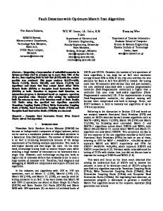
Figure 1: Observed measurements of system.
The initial conditions are set as
Algorithm 6 (fault detection using a variant Kalman filter). The initial conditions 𝑥0|0 and 𝑃0|0 are given. Step 1. Compute 𝑥𝑘|𝑘−1 and 𝑃𝑘|𝑘−1 using (12) and (13). Step 2. Compute 𝐸(Γ𝑘 ), 𝐸(𝐻𝑘 ), 𝐸(𝑦𝑘 ), and Var(𝑦𝑘 ) using (25), (26), (9), and (10). Step 3. Compute 𝑅𝑥̃𝑦̃ 𝑘 and 𝑅𝑦̃ 𝑦̃ 𝑘 using (27) and (28). Step 4. Compute 𝐾𝑘 using (21). Step 5. Compute 𝑥𝑘|𝑘 and 𝑃𝑘|𝑘 using (14) and (30). ̂ 𝑘 using (32) and then obtain 𝑟𝑘 through Step 6. Compute 𝑦 (33). Step 7. Evaluate 𝑟𝑘 using (34) and then compare it with the threshold using the rule (36). Step 8. Return to Step 1.
5. Simulation Results In this section, the simulation result will illustrate the applicability of the fault detection filter using the variant Tobit Kalman filtering. Consider the tracking system of ballistic roll rates explored in [32], which has the dynamic model of (2) with the state-space matrices: cos (𝜔) −sin (𝜔) 𝐴 = 𝛼[ ], sin (𝜔) cos (𝜔)
(37)
𝐶 = [1 0] . In this example, 𝛼 = 1; the frequency 𝜔 = 0.005 × 2𝜋; the standard deviation of process noise 𝑤𝑘 is 0.05; the variance of measurement noise V𝑘 is 1. The dead-zone of measurement is given as 0.2 (𝐶𝑥𝑘 + V𝑘 − 3) , 𝑦𝑘∗ ≥ 3, { { { { 𝑦𝑘 = 𝐷 (𝑦𝑘∗ ) = {0, −6 < 𝑦𝑘∗ < 3, (38) { { { ∗ {0.3 (𝐶𝑥𝑘 + V𝑘 + 6) , 𝑦𝑘 ≤ −6; that is, ℎ𝑟 = 0.2, ℎ𝑙 = 0.3, 𝑇𝑟 = 3, and 𝑇𝑙 = −6.
800 1000 1200 1400 1600 1800 2000
5 𝑥0 = [ ] , 0 1 0 ]. 𝑃0 = [ 0 1
(39)
Then, an intermittent fault is added to the system, which is described as follows: 1, { { { { { { {1.2, 𝑓𝑘 = { { { 1, { { { { {0,
500 ≤ 𝑘 ≤ 600, 880 ≤ 𝑘 ≤ 1000, 1600 ≤ 𝑘 ≤ 1700,
(40)
otherwise,
with coefficient matrix −0.1
𝐵=[
0.2
].
(41)
The simulation results are shown in Figures 1, 2, and 3. Figure 1 is the figure of the measurements with the deadzone. It can be seen that some parts of measurements have distortion or cannot be observed because of the dead-zone. Figure 2 presents the estimates of the processing states. The blue curve represents the true states and the red dash curve represents the estimates of states using the variant Kalman filter. Even though the data are absent or distorted, the estimation values of states using the variant Tobit Kalman filter can closely track the true states in fault-free case. When the faults occur, the difference between the true states and their estimates is obvious. Accordingly, the outputs of the variant Tobit Kalman filter provide accurate estimation of the measurements to generate the residual signal. Figure 3 illustrates 𝑓𝑘 , residual response, and residual evaluation function response varying with time 𝑘. The faults occur in the time intervals [500, 600], [880, 1000],
Journal of Control Science and Engineering
7
40
Table 1: Statistical performance.
xk (1)
20
Threshold FDT FAR (%) MAR (%)
0 −20 −40
0
200
400
600
xk (2)
20 0 −20 0
200
400
600
800 1000 1200 1400 1600 1800 2000
True state Variant Tobit Kalman
fk
Figure 2: Estimation of states.
Residual response
0.2223 699 9 7.67
0.2625 718 1.67 8.67
0.3492 761 0 42
missing alarm rate (MAR) is the probability of missing detection. It can be seen that the value of threshold can influence a lot the FDT, FAR, and MAR. As the value of threshold is becoming larger, it takes more time to detect the fault and raise alarm. The smaller threshold can reduce the MAR. However, the FAR is increasing at the same time. When threshold is chosen as a large value, although there will be less or even no false alarms, more faults will be failed to detect. Therefore, it is significant to choose a proper value of threshold and make a tradeoff among the FDT, FAR, and MAR.
2
6. Conclusion
1
In this paper, we have investigated the problem of fault detection for the discrete-time systems with output deadzone. Two Bernoulli random variables are introduced to describe the dead-zone of measurements. The variant Tobit Kalman filter is utilized for designing a recursive fault detection filter under the situation of dead-zone measurements. A simulation example of the occurrence of intermittent faults is provided. The simulation results have illustrated that the performance of fault detection filter is satisfied, where the fault can be recognized quickly and accurately. Also, the statistical performance of the fault detection method illustrated the relationship of threshold, FDT, FAR, and MAR. The dead-zone is a common issue arising in the engineering applications. The fault detection filter using the variant Tobit Kalman filter shows its practical value, with the good performance and lower computational expense. Furthermore, it can be extended to the fault detection for twodimension systems like vision-based systems with occlusion region.
0
0
200
400
600
800 1000 1200 1400 1600 1800 2000
0
200
400
600
800 1000 1200 1400 1600 1800 2000
0
200
400
600
800 1000 1200 1400 1600 1800 2000
2 0 −2
Residual evaluation
0.2144 694 13 5.67
800 1000 1200 1400 1600 1800 2000
40
−40
0.1846 688 61.67 3.67
2 1 0
Faulty Threshold
Figure 3: 𝑓𝑘 , residual response and residual evaluation.
Competing Interests and [1600, 1700] with the magnitude and coefficient matrix defined as (40) and (41). In the figure of residual evaluation, the blue curve is the response of faulty systems and the red dash line represents the preset threshold. Figure 3 indicates that the response raises an alarm opportunely when the faults happen at time 𝑘 = 500, 𝑘 = 880, and 𝑘 = 1600. When the faults disappear at times 𝑘 = 600, 𝑘 = 1000, and 𝑘 = 1700, the alarms go down rapidly. These simulation results demonstrate that the residual can detect the intermittent faults accurately. The Monte Carlo method is applied to obtain the statistical performance of the fault detection method proposed in this paper. The statistical performance is shown in Table 1. Fault detection time (FDT) represents the time when the occurrence of fault is detected and the alarm raises. False alarm rate (FAR) is the probability of false detection and
The authors declare that they have no competing interests.
Acknowledgments This work was supported by the National Natural Science Foundation of China under Grants 61473163, 61522309, and 61490701 and Tsinghua University Initiative Scientific Research Program.
References [1] X. Sun, H. J. Marquez, T. Chen, and M. Riaz, “An improved PCA method with application to boiler leak detection,” ISA Transactions, vol. 44, no. 3, pp. 379–397, 2005.
8 [2] D. Diallo, M. E. H. Benbouzid, D. Hamad, and X. Pierre, “Fault detection and diagnosis in an induction machine drive: a pattern recognition approach based on concordia stator mean current vector,” IEEE Transactions on Energy Conversion, vol. 20, no. 3, pp. 512–519, 2005. [3] J. Liu, “Shannon wavelet spectrum analysis on truncated vibration signals for machine incipient fault detection,” Measurement Science and Technology, vol. 23, no. 5, Article ID 055604, 2012. [4] S. M. El-Shal and A. S. Morris, “A fuzzy expert system for fault detection in statistical process control of industrial processes,” IEEE Transactions on Systems, Man and Cybernetics Part C: Applications and Reviews, vol. 30, no. 2, pp. 281–289, 2000. [5] B. Samanta, “Gear fault detection using artificial neural networks and support vector machines with genetic algorithms,” Mechanical Systems and Signal Processing, vol. 18, no. 3, pp. 625– 644, 2004. [6] L. B. Jack and A. K. Nandi, “Fault detection using support vector machines and artificial neural networks, augmented by genetic algorithms,” Mechanical Systems and Signal Processing, vol. 16, no. 2-3, pp. 373–390, 2002. [7] P. V. J. Rodr´ıguez, M. Negrea, and A. Arkkio, “A simplified scheme for induction motor condition monitoring,” Mechanical Systems and Signal Processing, vol. 22, no. 5, pp. 1216–1236, 2008. [8] S. X. Ding, Model-based Fault Diagnosis Techniques: Design Schemes, Algorithms, and Tools, Springer, London, UK, 2nd edition, 2013. [9] Z. Gao, X. Liu, and M. Z. Q. Chen, “Unknown input observerbased robust fault estimation for systems corrupted by partially decoupled disturbances,” IEEE Transactions on Industrial Electronics, vol. 63, no. 4, pp. 2537–2547, 2016. [10] L. Wu, X. Yao, and W. X. Zheng, “Generalized 𝐻2 fault detection for two-dimensional Markovian jump systems,” Automatica, vol. 48, no. 8, pp. 1741–1750, 2012. [11] S. Tong, B. Huo, and Y. Li, “Observer-based adaptive decentralized fuzzy fault-tolerant control of nonlinear large-scale systems with actuator failures,” IEEE Transactions on Fuzzy Systems, vol. 22, no. 1, pp. 1–15, 2014. [12] S. Tong, T. Wang, and Y. Li, “Fuzzy adaptive actuator failure compensation control of uncertain stochastic nonlinear systems with unmodeled dynamics,” IEEE Transactions on Fuzzy Systems, vol. 22, no. 3, pp. 563–574, 2014. [13] H. J. Yang, Y. Q. Xia, and B. Liu, “Fault detection for T-S fuzzy discrete systems in finite-frequency domain,” IEEE Transactions on Systems, Man, and Cybernetics, Part B: Cybernetics, vol. 41, no. 4, pp. 911–920, 2011. [14] J. Blesa, P. Jim´enez, D. Rotondo, F. Nejjari, and V. Puig, “An interval NLPV parity equations approach for fault detection and isolation of a wind farm,” IEEE Transactions on Industrial Electronics, vol. 62, no. 6, pp. 3794–3805, 2015. [15] S. Tornil-Sin, C. Ocampo-Martinez, V. Puig, and T. Escobet, “Robust fault diagnosis of nonlinear systems using interval constraint satisfaction and analytical redundancy relations,” IEEE Transactions on Systems, Man, and Cybernetics: Systems, vol. 44, no. 1, pp. 18–29, 2014. [16] R. Isermann, “Fault diagnosis of machines via parameter estimation and knowledge processing—tutorial paper,” Automatica. A Journal of IFAC, the International Federation of Automatic Control, vol. 29, no. 4, pp. 815–835, 1993. [17] J.-A. Jiang, J.-Z. Yang, Y.-H. Lin, C.-W. Liu, and J.-C. Ma, “An adaptive PMU based fault detection/location technique for transmission lines part I: theory and algorithms,” IEEE Transactions on Power Delivery, vol. 15, no. 2, pp. 486–493, 2000.
Journal of Control Science and Engineering [18] X. He, Z. Wang, Y. Liu, and D. H. Zhou, “Least-squares fault detection and diagnosis for networked sensing systems using a direct state estimation approach,” IEEE Transactions on Industrial Informatics, vol. 9, no. 3, pp. 1670–1679, 2013. [19] X. He, Z. Wang, X. Wang, and D. H. Zhou, “Networked strong tracking filtering with multiple packet dropouts: algorithms and applications,” IEEE Transactions on Industrial Electronics, vol. 61, no. 3, pp. 1454–1463, 2014. [20] X. He, Z. Wang, L. Qin, and D. Zhou, “Active fault-tolerant control for an internet-based networked three-tank system,” IEEE Transactions on Control Systems Technology, vol. 24, no. 6, pp. 2150–2157, 2016. [21] R. E. Kalman, “A new approach to linear filtering and prediction problems,” Journal of Basic Engineering, vol. 82, no. 1, pp. 35–45, 1960. [22] D.-H. Zhou, J.-T. Shi, and X. He, “Review of intermittent fault diagnosis techniques for dynamic systems,” Acta Automatica Sinica, vol. 40, no. 2, pp. 161–171, 2014. [23] M. Chen, G. Xu, R. Yan, S. X. Ding, and D. Zhou, “Detecting scalar intermittent faults in linear stochastic dynamic systems,” International Journal of Systems Science, vol. 46, no. 8, pp. 1337– 1348, 2015. [24] X. He, Y. Hu, and K. Peng, “Intermittent fault detection for uncertain networked systems,” Mathematical Problems in Engineering, vol. 2013, Article ID 282168, 10 pages, 2013. [25] R. Yan, X. He, and D. Zhou, “Detection of intermittent faults for linear stochastic systems subject to time-varying parametric perturbations,” IET Control Theory & Applications, vol. 10, no. 8, pp. 903–910, 2016. [26] G. Tao and P. V. Kokotovic, “Adaptive control of plants with unknown dead-zones,” Institute of Electrical and Electronics Engineers. Transactions on Automatic Control, vol. 39, no. 1, pp. 59–68, 1994. [27] G. Tao and P. V. Kokotovi´c, “Discrete-time adaptive control of systems with unknown deadzones,” International Journal of Control, vol. 61, no. 1, pp. 1–17, 1995. [28] H. Cho and E.-W. Bai, “Convergence results for an adaptive dead zone inverse,” International Journal of Adaptive Control and Signal Processing, vol. 12, no. 5, pp. 451–466, 1998. [29] F. L. Lewis, W. K. Tim, L.-Z. Wang, and Z. X. Li, “Deadzone compensation in motion control systems using adaptive fuzzy logic control,” IEEE Transactions on Control Systems Technology, vol. 7, no. 6, pp. 731–742, 1999. [30] R. R. Selmic and F. L. Lewis, “Deadzone compensation in motion control systems using neural networks,” Institute of Electrical and Electronics Engineers. Transactions on Automatic Control, vol. 45, no. 4, pp. 602–613, 2000. [31] J. Tobin, “Estimation of relationships for limited dependent variables,” Econometrica, vol. 26, no. 1, pp. 24–36, 1958. [32] B. Allik, C. Miller, M. J. Piovoso, and R. Zurakowski, “The Tobit Kalman filter: an estimator for censored measurements,” IEEE Transactions on Control Systems Technology, vol. 24, no. 1, pp. 365–371, 2016. [33] B. Allik, C. Miller, M. J. Piovoso, and R. Zurakowski, “Nonlinear estimators for censored data: a comparison of the EKF, the UKF and the Tobit Kalman filter,” in Proceedings of the 2015 American Control Conference (ACC ’15), pp. 5146–5151, Chicago, Ill, USA, July 2015. [34] C. Andrieu and A. Doucet, “Particle filtering for partially observed Gaussian state space models,” Journal of the Royal Statistical Society. Series B. Statistical Methodology, vol. 64, no. 4, pp. 827–836, 2002.
Journal of Control Science and Engineering [35] C. Snyder, T. Bengtsson, P. Bickel, and J. Anderson, “Obstacles to high-dimensional particle filtering,” Monthly Weather Review, vol. 136, no. 12, pp. 4629–4640, 2008. [36] M. Chen, B. Jiang, and W. W. Guo, “Fault-tolerant control for a class of non-linear systems with dead-zone,” International Journal of Systems Science, vol. 47, no. 7, pp. 1689–1699, 2016. [37] M. Chen and G. Tao, “Adaptive fault-tolerant control of uncertain nonlinear large-scale systems with unknown dead zone,” IEEE Transactions on Cybernetics, vol. 46, no. 8, pp. 1851–1862, 2016.
9
International Journal of
Rotating Machinery
Engineering Journal of
Hindawi Publishing Corporation http://www.hindawi.com
Volume 2014
The Scientific World Journal Hindawi Publishing Corporation http://www.hindawi.com
Volume 2014
International Journal of
Distributed Sensor Networks
Journal of
Sensors Hindawi Publishing Corporation http://www.hindawi.com
Volume 2014
Hindawi Publishing Corporation http://www.hindawi.com
Volume 2014
Hindawi Publishing Corporation http://www.hindawi.com
Volume 2014
Journal of
Control Science and Engineering
Advances in
Civil Engineering Hindawi Publishing Corporation http://www.hindawi.com
Hindawi Publishing Corporation http://www.hindawi.com
Volume 2014
Volume 2014
Submit your manuscripts at https://www.hindawi.com Journal of
Journal of
Electrical and Computer Engineering
Robotics Hindawi Publishing Corporation http://www.hindawi.com
Hindawi Publishing Corporation http://www.hindawi.com
Volume 2014
Volume 2014
VLSI Design Advances in OptoElectronics
International Journal of
Navigation and Observation Hindawi Publishing Corporation http://www.hindawi.com
Volume 2014
Hindawi Publishing Corporation http://www.hindawi.com
Hindawi Publishing Corporation http://www.hindawi.com
Chemical Engineering Hindawi Publishing Corporation http://www.hindawi.com
Volume 2014
Volume 2014
Active and Passive Electronic Components
Antennas and Propagation Hindawi Publishing Corporation http://www.hindawi.com
Aerospace Engineering
Hindawi Publishing Corporation http://www.hindawi.com
Volume 2014
Hindawi Publishing Corporation http://www.hindawi.com
Volume 2014
Volume 2014
International Journal of
International Journal of
International Journal of
Modelling & Simulation in Engineering
Volume 2014
Hindawi Publishing Corporation http://www.hindawi.com
Volume 2014
Shock and Vibration Hindawi Publishing Corporation http://www.hindawi.com
Volume 2014
Advances in
Acoustics and Vibration Hindawi Publishing Corporation http://www.hindawi.com
Volume 2014